
Physics-Informed Graph Neural Networks for Attack Path Prediction


Abstract
1. Introduction
| (RQ) Can adversary behavior be generalized across multiple environments to achieve full path prediction accuracy comparable to SoTA exploit prediction methods ? |
2. Materials and Methods
2.1. Dataset
2.1.1. Realistic Attacks and Environments
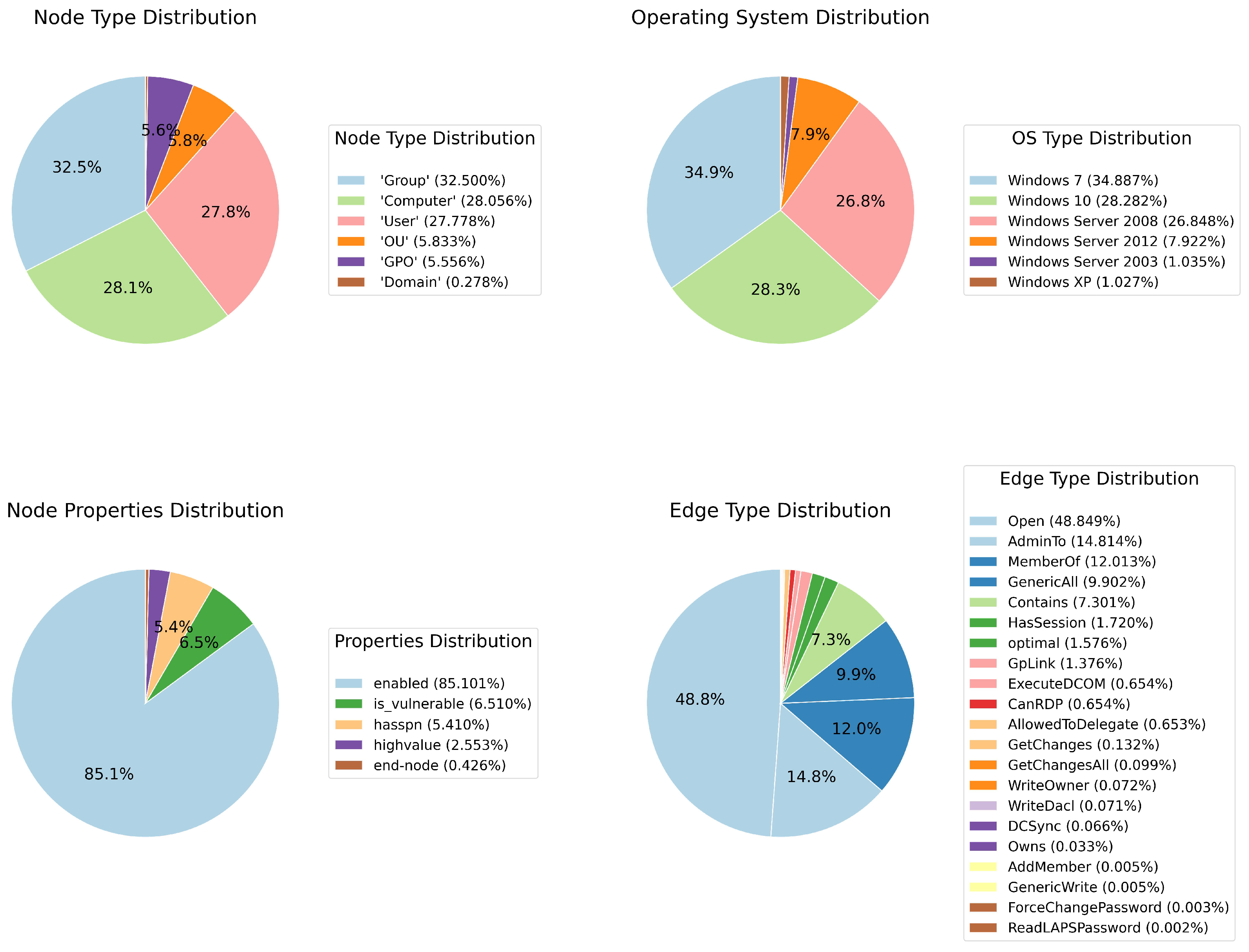
2.1.2. Exploratory Data Analysis
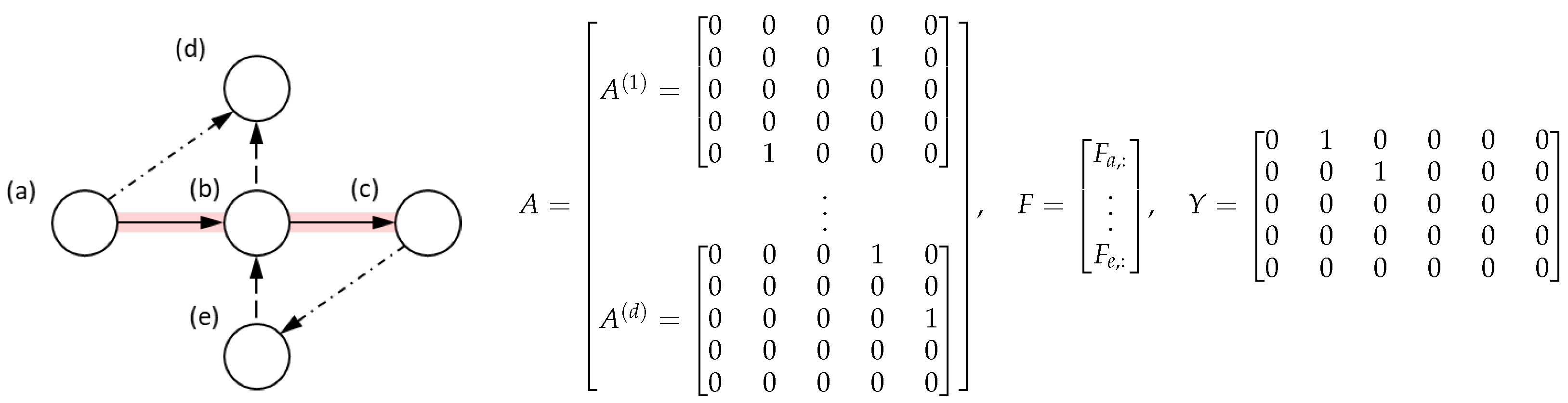
2.1.3. Data Structure for Learning
2.2. Physics-Informed Learning
| In the context of attack path prediction across high-dimensional environments, using PINNs instead of agnostic Deep Neural Networks presents two key advantages: (1) incorporating known interaction principles and properties into the training restricts the space of feasible learnable solutions and thereby enhances the generalizability of the function approximation, and (2) by embedding this prior knowledge, PINNs also effectively augment the information content of the available data, enabling convergence towards accurate solutions with a limited number of training samples. |
2.3. Formal Problem Setting
|
2.4. Architecture
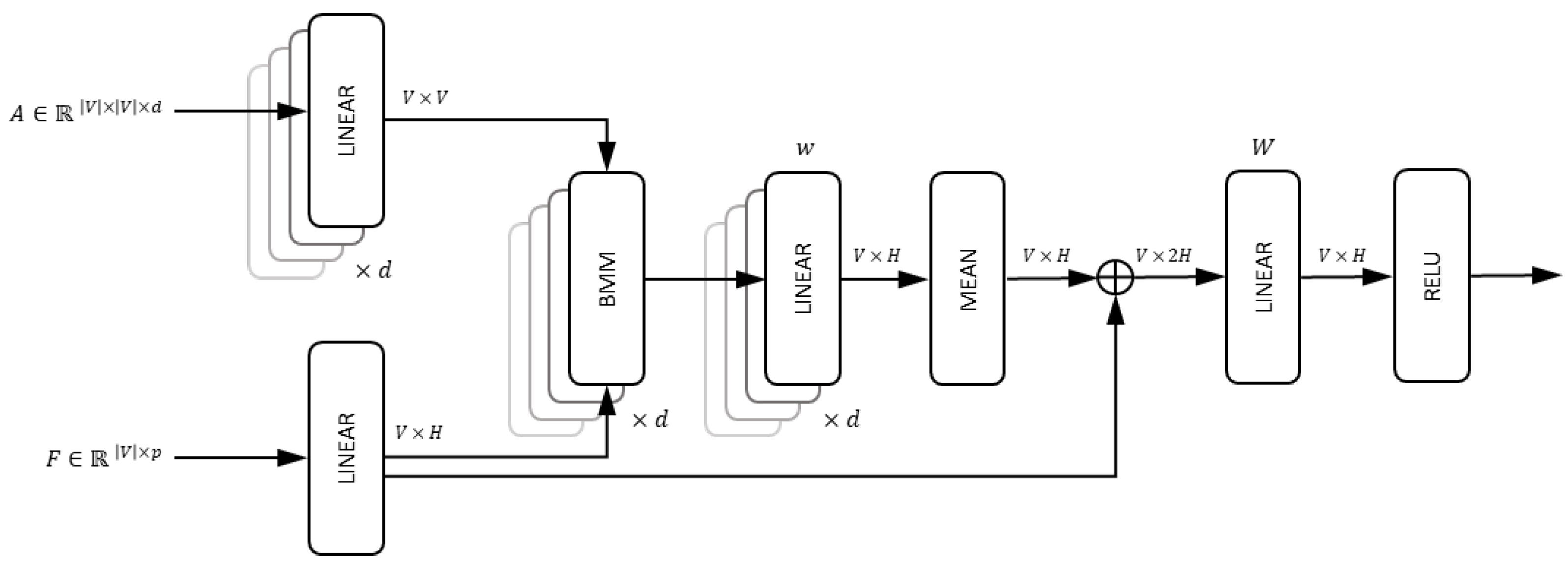
2.4.1. Graph Convolution Block
| Algorithm 1 Inference with BMM SAGEConv layer |
|
| The BMM SAGEConv layer k, given , can be written compactly as follows: |
2.4.2. Path Prediction Task
2.4.3. Node Classification Task
2.5. Path Prediction Training
2.5.1. Data Loss
2.5.2. Physics-Inspired Loss
2.5.3. Degree Component
| The degree component ensures that the predicted graph follows a structured, single-path format without branches. This is achieved by analyzing the in-degree and out-degree of each node in the active set, which represent the number of incoming and outgoing connections, respectively. If multiple nodes are identified as potential starting points (having no incoming edges) or multiple nodes are seen as ending points (having no outgoing edges), the model is penalized, and parameters are updated accordingly. Additionally, intermediary nodes should have exactly one incoming and one outgoing connection to maintain a proper sequence. The loss function sums up these penalties across all graphs in a batch, ensuring the network consistently learns to predict non-branching paths. |
2.5.4. Cycle Component
| The cycle component prevents the presence of loops in the predicted graph. A cycle means that one can start from a node, follow the connections, and return to the same node. This is undesirable in our context, so the model is penalized if cycles are detected. Mathematically, this is achieved using the adjacency matrix of the graph: by raising this matrix to successive powers, we can count the number of paths of different lengths. If a sum of these paths indicates a cycle, a penalty is applied. This ensures that the predicted structure is strictly forward-moving, preventing redundant or circular paths. |
2.5.5. Connectivity Component
| The connectivity component ensures that the predicted graph consists of a single connected path rather than multiple disconnected segments. This is achieved using the Laplacian matrix, which describes the structure of the graph. The eigenvalues of this matrix provide information about how connected the graph is: in particular, the number of zero eigenvalues indicates how many separate components exist. If the number of components does not match the expected value for a properly connected path, the model is penalized. Additionally, spectral graph theory tells us the expected eigenvalues for an ideal path graph, so a second penalty is added if the observed eigenvalues deviate from this expected pattern. By enforcing these constraints, the model learns to generate graphs that form a single continuous sequence without fragmentation. |
2.6. Start/End Node Training
2.6.1. Encoder Self-Supervised Training
2.6.2. Classifier Supervised Training
3. Results
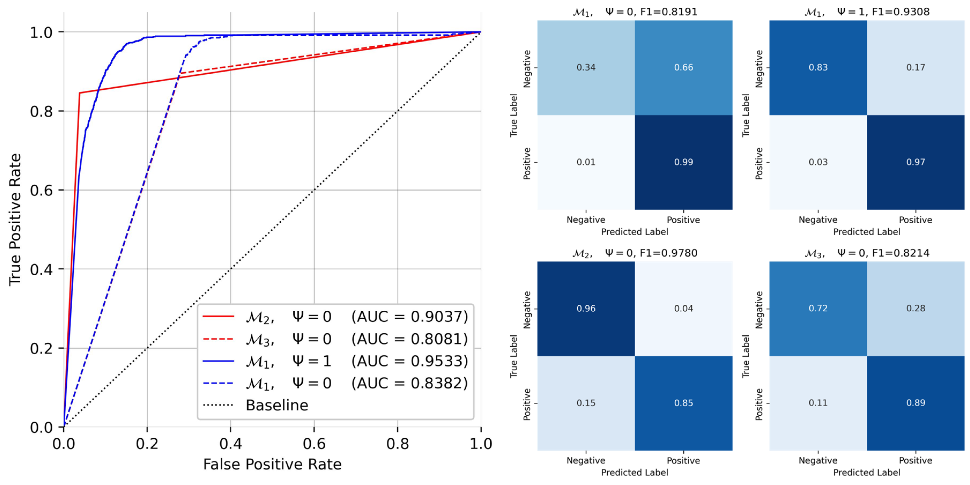
3.1. Evaluation
| For path prediction (), we obtained a final evaluation F1 score of and ROC-AUC , which is superior to the EPSS performance. For start/end node classification (), we obtained an F1 score of and ROC-AUC of for start node prediction and F1 score of and ROC-AUC for end node prediction. |
3.2. Ablation Study
3.3. Sensitivity Analysis
4. Discussion
5. Conclusions
Author Contributions
Funding
Data Availability Statement
Conflicts of Interest
Appendix A. Summary of Statistics


| Num_Nodes | Num_Edges | Density | Avg_Degree | Median_Degree | Max_Degree | |
|---|---|---|---|---|---|---|
| count | 1033 | 1033 | 1033 | 1033 | 1033 | 1033 |
| mean | 361.0 | 3040.83 | 0.0234 | 16.85 | 5.88 | 423.89 |
| std | 0.0 | 90.19 | 0.0007 | 0.50 | 0.32 | 3.27 |
| min | 361.0 | 2755 | 0.0212 | 15.26 | 5 | 414 |
| 25% | 361.0 | 2979 | 0.0229 | 16.50 | 6 | 422 |
| 50% | 361.0 | 3043 | 0.0234 | 16.86 | 6 | 424 |
| 75% | 361.0 | 3102 | 0.0239 | 17.19 | 6 | 426 |
| max | 361.0 | 3288 | 0.0253 | 18.22 | 6 | 437 |
Appendix B. K-Fold Cross Validation
Appendix C. F1 Score
Appendix D. ROC-AUC Measure
Appendix E. Complexity Analysis
Appendix E.1. Path Prediction Architecture
| Listing A1. implementation. |
| class BMMSageConvLayer(nn.Module): … def message_passing(self, x: torch.Tensor, adj_tensor: torch.Tensor): batch_size, num_nodes, _ = x.shape aggregated_neigh_embeds = [] for i in range(adj_tensor.shape[3]): adj_matrix = adj_tensor[:, :, :, i] neigh_embeds_i = torch.bmm(adj_matrix, x) neigh_embeds_i = self.lin_neighbors[i](neigh_embeds_i) aggregated_neigh_embeds.append(neigh_embeds_i) neigh_embeds = sum(aggregated_neigh_embeds) return neigh_embeds def forward(self, x: torch.Tensor, adj_tensor: torch.Tensor): neigh_embeds = self.message_passing(x, adj_tensor) x_self = self.lin_self(x) out = neigh_embeds + x_self return self.act(out) class DNN(nn.Module): … def forward(self, x): x = F.relu(self.fc1(x)) … x = torch.sigmoid(self.fc5(x)) return x |
Appendix E.2. Node Classification Architecture
| Listing A2. implementation. |
| class AE(torch.nn.Module): … def forward(self, x): encoded = self.encoder(x) decoded = self.decoder(encoded) return decoded … class EncoderWithClassifier(nn.Module): … def forward(self, x, adj_tensor): batch_size, num_nodes, _ = x.shape node_embeddings = self.graphsage(x, adj_tensor) … latent_repr = self.encoder(node_embeddings)s classification_output = self.classifier(latent_repr) … return classification_output |
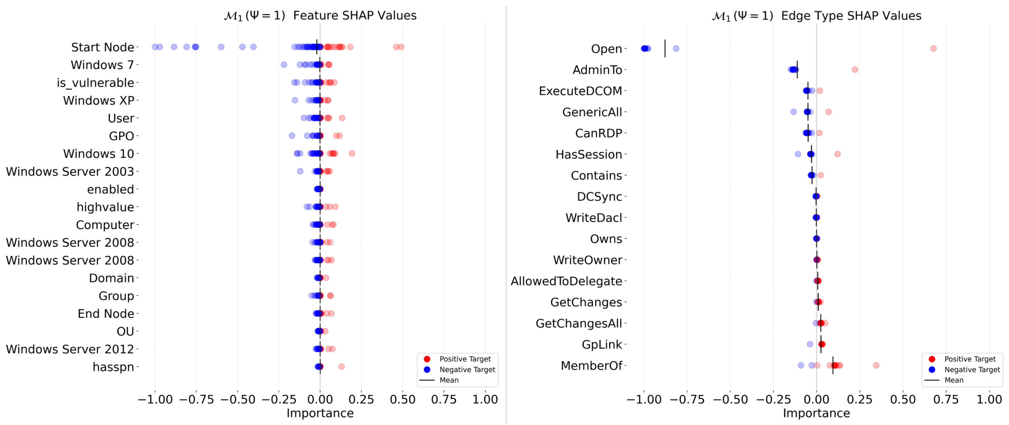
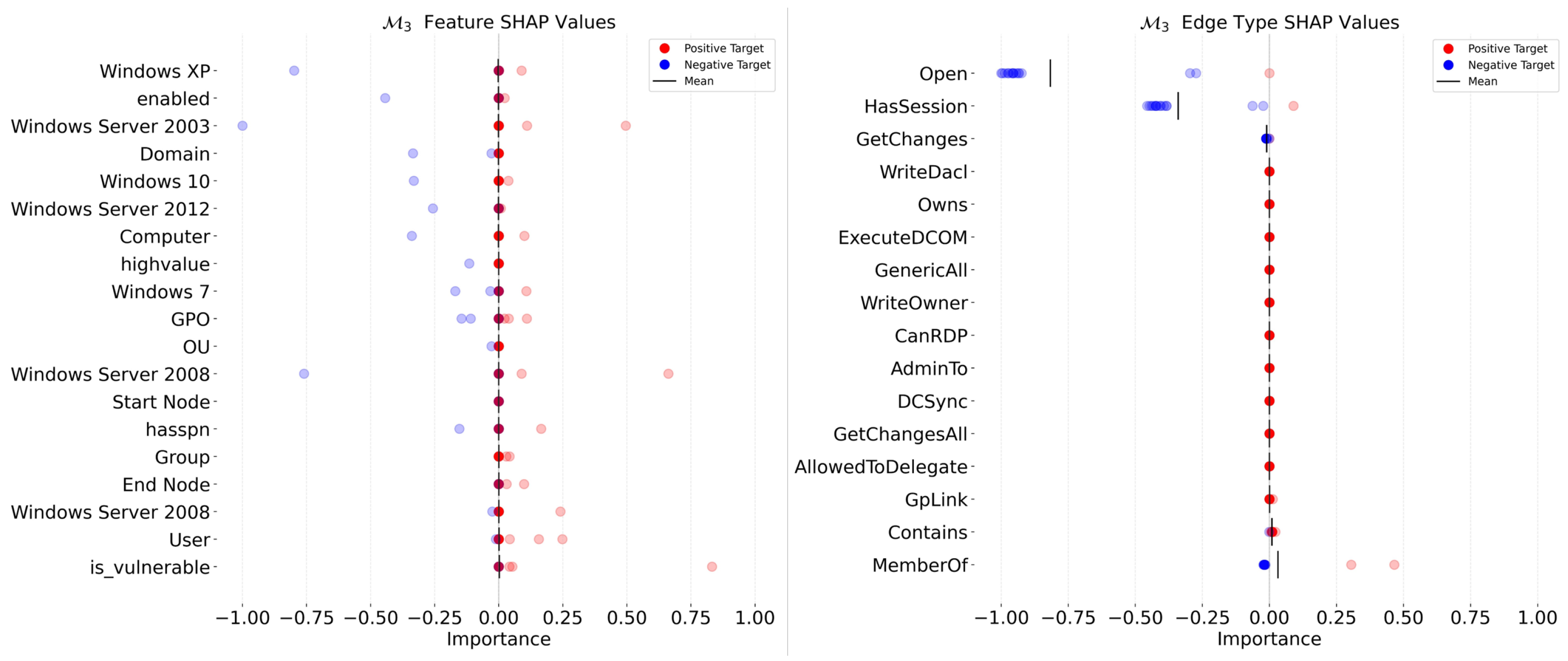
Appendix F. Shapley Additive Explanations (SHAP)
References
- Minden, S.L.; Henderson, M. From information to a system. Behav. Healthc. Tomorrow 2000, 9, 31–33. [Google Scholar] [PubMed]
- Servigne, S. Conception, architecture et urbanisation des systèmes d’information. In Encyclopædia Universalis; Encyclopædia Universalis: Boulogne-Billancour, France, 2010; pp. 1–15. [Google Scholar]
- Yu, E.S.K. Information Systems. In The Practical Handbook of Internet Computing; Chapman and Hall/CRC: London, UK, 2004. [Google Scholar]
- Eling, M.; McShane, M.; Nguyen, T. Cyber risk management: History and future research directions. Risk Manag. Insur. Rev. 2021, 24, 93–125. [Google Scholar] [CrossRef]
- Alavi, M.; Weiss, I.R. Managing the risks associated with end-user computing. J. Manag. Inf. Syst. 1985, 2, 5–20. [Google Scholar] [CrossRef]
- Rainer, R.K., Jr.; Snyder, C.A.; Carr, H.H. Risk analysis for information technology. J. Manag. Inf. Syst. 1991, 8, 129–147. [Google Scholar] [CrossRef]
- Eloff, J.H.; Labuschagne, L.; Badenhorst, K.P. A comparative framework for risk analysis methods. Comput. Secur. 1993, 12, 597–603. [Google Scholar] [CrossRef]
- Whitman, M.E.; Mattord, H.J. Principles of Information Security; Thomson Course Technology: Boston, MA, USA, 2009. [Google Scholar]
- Naik, N.; Jenkins, P.; Grace, P.; Song, J. Comparing attack models for IT systems: Lockheed Martin’s Cyber Kill Chain, MITRE ATT&CK Framework and Diamond Model. In Proceedings of the 2022 IEEE International Symposium on Systems Engineering (ISSE), Vienna, Austria, 24–26 October 2022; pp. 1–7. [Google Scholar]
- Elmiger, M.; Lemoudden, M.; Pitropakis, N.; Buchanan, W.J. Start thinking in graphs: Using graphs to address critical attack paths in a Microsoft cloud tenant. Int. J. Inf. Secur. 2024, 23, 467–485. [Google Scholar] [CrossRef]
- Dunagan, J.; Zheng, A.X.; Simon, D.R. Heat-ray: Combating identity snowball attacks using machinelearning, combinatorial optimization and attack graphs. In Proceedings of the ACM SIGOPS 22nd Symposium on Operating Systems Principles, Big Sky, MT, USA, 11–14 October 2009; pp. 305–320. [Google Scholar]
- Irfan, A.N.; Chuprat, S.; Mahrin, M.N.; Ariffin, A. Taxonomy of cyber threat intelligence framework. In Proceedings of the 2022 13th International Conference on Information and Communication Technology Convergence (ICTC), Jeju Island, Republic of Korea, 19–21 October 2022; pp. 1295–1300. [Google Scholar]
- Cohen, F. Simulating cyber attacks, defences, and consequences. Comput. Secur. 1999, 18, 479–518. [Google Scholar] [CrossRef]
- Kuhl, M.E.; Sudit, M.; Kistner, J.; Costantini, K. Cyber attack modeling and simulation for network security analysis. In Proceedings of the 2007 Winter Simulation Conference, Washington, DC, USA, 9–12 December 2007; pp. 1180–1188. [Google Scholar]
- Abraham, S.; Nair, S. A Novel Architecture for Predictive CyberSecurity Using Non-Homogenous Markov Models. 2015. Available online: https://ieeexplore.ieee.org/document/7345354 (accessed on 7 April 2025).
- Woodard, M.; Marashi, K.; Sarvestani, S.S.; Hurson, A.R. Survivability evaluation and importance analysis for cyber–physical smart grids. Reliab. Eng. Syst. Saf. 2021, 210, 107479. [Google Scholar] [CrossRef]
- Holm, H.; Shahzad, K.; Buschle, M.; Ekstedt, M. P2CySeMoL: Predictive, Probabilistic Cyber Security Modeling Language. IEEE Trans. Dependable Secur. Comput. 2014, 12, 626–639. [Google Scholar] [CrossRef]
- Holm, H.; Shahzad, K.; Buschle, M. P2 CySeMoL: Predictive, Probabilistic Cyber Security Modeling Language (No Date). Available online: https://ieeexplore.ieee.org/document/6990572 (accessed on 7 April 2025).
- Holm, H.; Shahzad, K.; Buschle, M. Quantifying & Minimizing Attack Surfaces Containing Moving Target Defenses. 2015. Available online: http://ieeexplore.ieee.org/document/7287449 (accessed on 7 April 2025).
- Hong, J.B.; Kim, D.S.; Haqiq, A. What Vulnerability Do We Need to Patch First? Available online: https://ieeexplore.ieee.org/document/6903625 (accessed on 7 April 2025).
- Lippmann, R.P.; Ingols, K.W. An Annotated Review of Past Papers on Attack Graphs; MIT Lincoln Laboratory: Lexington, MA, USA, 2005. [Google Scholar]
- Valja, M.; Korman, M.; Shahzad, K. Integrated Metamodel for Security Analysis, IEEE Xplore Login (No Date A). Available online: http://ieeexplore.ieee.org/docurnent/7070437 (accessed on 7 April 2025).
- Yu, Y.; Si, X.; Hu, C.; Zhang, J. A review of recurrent neural networks: LSTM cells and network architectures. Neural Comput. 2019, 31, 1235–1270. [Google Scholar] [CrossRef]
- Yusuf, S.E.; Mengmeng, G.; Hong, J.B. Security Modelling and Analysis of Dynamic Enterprise Networks. 2016. Available online: http://ieeexplore.ieee.org/stamp/stamp.jsp?arnumber=7876345 (accessed on 7 April 2025).
- Ekin, T. Augmented Probability Simulation Methods for Non-Cooperative Games. Available online: https://arxiv.org/abs/1910.04574 (accessed on 7 April 2025).
- Miller, S.; Wagner, C.; Aickelin, U.; Garibaldi, J.M. Modelling Cyber-Security Experts’ Decision Making Processes using Aggre-gation Operators. arXiv 2016, arXiv:1608.08497. [Google Scholar] [CrossRef]
- Applebaum, A.; Miller, D.; Strom, B.; Korban, C.; Wolf, R. Intelligent, automated red team emulation. In Proceedings of the Annual Computer Security Applications Conference, ACSAC, Los Angeles, CA, USA, 5–9 December 2016; pp. 363–373. [Google Scholar]
- Miller, H.; Griffy-Brown, C. Developing a Framework and Methodology for Assessing Cyber Risk for Business Leaders. J. Appl. Bus. Econ. 2018, 20, 34–50. [Google Scholar]
- Sarraute, C.; Buffet, O.; Hoffmann, J. POMDPs make better hackers: Accounting for uncertainty in penetration testing. In Proceedings of the AAAI Conference on Artificial Intelligence, AAAI, Toronto, ON, Canada, 22–26 July 2012; Volume 26, pp. 1816–1824. [Google Scholar]
- Molina-Markham, A.; Winder, R.K.; Ridley, A. Network defense is not a game. arXiv 2021, arXiv:2104.10262. [Google Scholar]
- Goel, D.; Ward-Graham, M.H.; Neumann, A.; Neumann, F.; Nguyen, H.; Guo, M. Defending active directory by combining neural network based dynamic program and evolutionary diversity optimisation. In Proceedings of the Genetic and Evolutionary Computation Conference, Boston, MA, USA, 9–13 July 2022; pp. 1191–1199. [Google Scholar]
- Han, Y.; Rubinstein, B.I.; Abraham, T.; Alpcan, T.; De Vel, O.; Erfani, S.; Hubczenko, D.; Leckie, C.; Montague, P. Reinforcement learning for autonomous defence in software-defined networking. In Proceedings of the Decision and Game Theory for Security: 9th International Conference, GameSec 2018, Seattle, WA, USA, 29–31 October 2018; Proceedings 9. Springer: Berlin/Heidelberg, Germany, 2018; pp. 145–165. [Google Scholar]
- Han, Y.; Hubczenko, D.; Montague, P.; De Vel, O.; Abraham, T.; Rubinstein, B.I.; Leckie, C.; Alpcan, T.; Erfani, S. Adversarial reinforcement learning under partial observability in autonomous computer network defence. In Proceedings of the 2020 International Joint Conference on Neural Networks (IJCNN), Glasgow, UK, 19–24 July 2020; pp. 1–8. [Google Scholar]
- Baillie, C.; Standen, M.; Schwartz, J.; Docking, M.; Bowman, D.; Kim, J. Cyborg: An autonomous cyber operations research gym. arXiv 2020, arXiv:2002.10667. [Google Scholar]
- Dhir, N.; Hoeltgebaum, H.; Adams, N.; Briers, M.; Burke, A.; Jones, P. Prospective artificial intelligence approaches for active cyber defence. arXiv 2021, arXiv:2104.09981. [Google Scholar]
- Gangupantulu, R.; Cody, T.; Park, P.; Rahman, A.; Eisenbeiser, L.; Radke, D.; Clark, R.; Redino, C. Using cyber terrain in reinforcement learning for penetration testing. In Proceedings of the 2022 IEEE International Conference on Omni-layer Intelligent Systems (COINS), Barcelona, Spain, 1–3 August 2022; pp. 1–8. [Google Scholar]
- Li, L.; Fayad, R.; Taylor, A. Cygil: A cyber gym for training autonomous agents over emulated network systems. arXiv 2021, arXiv:2109.03331. [Google Scholar]
- Andrew, A.; Spillard, S.; Collyer, J.; Dhir, N. Developing optimal causal cyber-defence agents via cyber security simulation. arXiv 2022, arXiv:2207.12355. [Google Scholar]
- Bradley, J.; Atkins, E. Toward continuous state—Space regulation of coupled cyber—Physical systems. Proc. IEEE 2011, 100, 60–74. [Google Scholar] [CrossRef]
- Zhang, J.; Guo, L.; Ye, J. Cyber-attack detection for photovoltaic farms based on power-electronics-enabled harmonic state space modeling. IEEE Trans. Smart Grid 2021, 13, 3929–3942. [Google Scholar] [CrossRef]
- He, R.; Xie, H.; Deng, J.; Feng, T.; Lai, L.; Shahidehpour, M. Reliability modeling and assessment of cyber space in cyber-physical power systems. IEEE Trans. Smart Grid 2020, 11, 3763–3773. [Google Scholar] [CrossRef]
- Yang, L.; Cao, X.; Li, J. A new cyber security risk evaluation method for oil and gas SCADA based on factor state space. Chaos, Solitons Fractals 2016, 89, 203–209. [Google Scholar] [CrossRef]
- Ajmal, A.B.; Shah, M.A.; Maple, C.; Asghar, M.N.; Islam, S.U. Offensive security: Towards proactive threat hunting via adversary emulation. IEEE Access 2021, 9, 126023–126033. [Google Scholar] [CrossRef]
- Ajmal, A.B.; Khan, S.; Alam, M.; Mehbodniya, A.; Webber, J.; Waheed, A. Toward effective evaluation of cyber defense: Threat based adversary emulation approach. IEEE Access 2023, 11, 70443–70458. [Google Scholar] [CrossRef]
- Yoo, J.D.; Park, E.; Lee, G.; Ahn, M.K.; Kim, D.; Seo, S.; Kim, H.K. Cyber attack and defense emulation agents. Appl. Sci. 2020, 10, 2140. [Google Scholar] [CrossRef]
- Eckhart, M.; Ekelhart, A. Digital twins for cyber-physical systems security: State of the art and outlook. In Security and Quality in Cyber-Physical Systems Engineering: With Forewords by Robert M. Lee and Tom Gilb; Springer: Cham, Switzerland, 2019; pp. 383–412. [Google Scholar]
- Dietz, M.; Vielberth, M.; Pernul, G. Integrating digital twin security simulations in the security operations center. In Proceedings of the 15th International Conference on Availability, Reliability and Security, Dublin, Ireland, 25–28 August 2020; pp. 1–9. [Google Scholar]
- Dietz, M.; Englbrecht, L.; Pernul, G. Enhancing industrial control system forensics using replication-based digital twins. In Proceedings of the Advances in Digital Forensics XVII: 17th IFIP WG 11.9 International Conference, Virtual Event, 1–2 February 2021; Revised Selected Papers 17. Springer: Berlin/Heidelberg, Germany, 2021; pp. 21–38. [Google Scholar]
- Homaei, M.; Gutiérrez, O.M.; Núñez, J.C.S.; Vegas, M.A.; Lindo, A.C. A Review of Digital Twins and their Application in Cybersecurity based on Artificial Intelligence. arXiv 2023, arXiv:2311.01154. [Google Scholar] [CrossRef]
- Suhail, S.; Iqbal, M.; Hussain, R.; Jurdak, R. ENIGMA: An explainable digital twin security solution for cyber–physical systems. Comput. Ind. 2023, 151, 103961. [Google Scholar] [CrossRef]
- Allison, D.; Smith, P.; Mclaughlin, K. Digital Twin-Enhanced Incident Response for Cyber-Physical Systems. In Proceedings of the 18th International Conference on Availability, Reliability and Security, Benevento, Italy, 29 July–1 August 2023; pp. 1–10. [Google Scholar]
- Empl, P.; Schlette, D.; Zupfer, D.; Pernul, G. SOAR4IoT: Securing IoT Assets with Digital Twins. In Proceedings of the 17th International Conference on Availability, Reliability and Security, Vienna, Austria, 23–26 August 2022; pp. 1–10. [Google Scholar]
- Coppolino, L.; Nardone, R.; Petruolo, A.; Romano, L.; Souvent, A. Exploiting digital twin technology for cybersecurity monitoring in smart grids. In Proceedings of the 18th International Conference on Availability, Reliability and Security, Benevento, Italy, 29 July–1 August 2023; pp. 1–10. [Google Scholar]
- François, M. GraphETL: Construction d’une plateforme versatile pour la modélisation du risque cyber. In Proceedings of the INFormatique des ORganisations et Systèmes d’Information et de Décision (INFORSID)—Forum JCJC, 42e édition, Nancy, France, 28–31 May 2024; pp. 105–120. [Google Scholar]
- François, M.; Arduin, P.E.; Merad, M. Artificial Intelligence & Cybersecurity: A Preliminary Study of Automated Pentesting with Offensive Artificial Intelligence. In Proceedings of the International Conference on Information and Knowledge Systems; Springer: Berlin/Heidelberg, Germany, 2021; pp. 131–138. [Google Scholar]
- François, M.; Arduin, P.E.; Merad, M. Classification of Decision Support Systems for Cybersecurity. In Proceedings of the 15th Mediterranean Conference on Information Systems (MCIS) and the 6th Middle East & North Africa Conference on digital Information Systems (MENACIS), Madrid, Spain, 6–9 September 2023. [Google Scholar]
- Jacobs, J.; Romanosky, S.; Suciu, O.; Edwards, B.; Sarabi, A. Enhancing Vulnerability Prioritization: Data-driven Exploit Predictions with Community-driven Insights. In Proceedings of the 2023 IEEE European Symposium on Security and Privacy Workshops (EuroS&PW), Delft, The Netherlands, 3–7 July 2023; pp. 194–206. [Google Scholar]
- FIRST. Common Vulnerability Scoring System. Available online: https://www.first.org/ (accessed on 7 April 2025).
- Jacobs, J.; Romanosky, S.; Edwards, B.; Adjerid, I.; Roytman, M. Exploit prediction scoring system (epss). Digit. Threat. Res. Pract. 2021, 2, 1–17. [Google Scholar] [CrossRef]
- Allodi, L.; Massacci, F. A preliminary analysis of vulnerability scores for attacks in wild: The ekits and sym datasets. In Proceedings of the 2012 ACM Workshop on Building Analysis Datasets and Gathering Experience Returns for Security, Raleigh, NC, USA, 15 October 2012; pp. 17–24. [Google Scholar]
- Allodi, L.; Massacci, F. Comparing vulnerability severity and exploits using case-control studies. ACM Trans. Inf. Syst. Secur. (TISSEC) 2014, 17, 1–20. [Google Scholar] [CrossRef]
- Younis, A.A.; Malaiya, Y.K. Comparing and evaluating CVSS base metrics and microsoft rating system. In Proceedings of the 2015 IEEE International Conference on Software Quality, Reliability and Security, Vancouver, BC, Canada, 3–5 August 2015; pp. 252–261. [Google Scholar]
- Suciu, O.; Nelson, C.; Lyu, Z.; Bao, T.; Dumitraș, T. Expected exploitability: Predicting the development of functional vulnerability exploits. In Proceedings of the 31st USENIX Security Symposium (USENIX Security 22), Boston, MA, USA, 10–12 August 2022; pp. 377–394. [Google Scholar]
- Goodfellow, I.; Bengio, Y.; Courville, A.; Bengio, Y. Deep Learning; MIT Press: Cambridge, MA, USA; Boston, MA, USA, 2016. [Google Scholar]
- Cybenko, G. Approximation by superpositions of a sigmoidal function. Math. Control Signals Syst. 1989, 2, 303–314. [Google Scholar] [CrossRef]
- François, M.; Arduin, P.; Merad, M. Latent States: Model Based Machine Learning Perspectives on Cyber Resilience. In Proceedings of the IEEE 4th Intelligent Cybersecurity Conference (ICSC), Valencia, Spain, 17–20 September 2024. [Google Scholar]
- Rahman, M.R.; Mahdavi-Hezaveh, R.; Williams, L. A literature review on mining cyberthreat intelligence from unstructured texts. In Proceedings of the 2020 International Conference on Data Mining Workshops (ICDMW), Virtual, 17–20 November 2020; pp. 516–525. [Google Scholar]
- Takko, T.; Bhattacharya, K.; Lehto, M.; Jalasvirta, P.; Cederberg, A.; Kaski, K. Knowledge mining of unstructured information: Application to cyber domain. Sci. Rep. 2023, 13, 1714. [Google Scholar] [CrossRef]
- Nguyen, T.T.; Reddi, V.J. Deep reinforcement learning for cyber security. IEEE Trans. Neural Netw. Learn. Syst. 2021, 34, 3779–3795. [Google Scholar] [CrossRef] [PubMed]
- Skopik, F.; Settanni, G.; Fiedler, R. A problem shared is a problem halved: A survey on the dimensions of collective cyber defense through security information sharing. Comput. Secur. 2016, 60, 154–176. [Google Scholar] [CrossRef]
- Sedenberg, E.M.; Dempsey, J.X. Cybersecurity information sharing governance structures: An ecosystem of diversity, trust, and tradeoffs. arXiv 2018, arXiv:1805.12266. [Google Scholar]
- Pala, A.; Zhuang, J. Information sharing in cybersecurity: A review. Decis. Anal. 2019, 16, 172–196. [Google Scholar] [CrossRef]
- Nolan, A. Cybersecurity and Information Sharing: Legal Challenges and Solutions; Congressional Research Service: Washington, DC, USA, 2015; Volume 5. [Google Scholar]
- Murdoch, S.; Leaver, N. Anonymity vs. trust in cyber-security collaboration. In Proceedings of the 2nd ACM Workshop on Information Sharing and Collaborative Security, Denver, CO, USA, 12 October 2015; pp. 27–29. [Google Scholar]
- Dandurand, L.; Serrano, O.S. Towards improved cyber security information sharing. In Proceedings of the 2013 5th International Conference on Cyber Conflict (CYCON 2013), Talinn, Estonia, 4–7 June 2013; pp. 1–16. [Google Scholar]
- Specter Ops BloodHound. 2024. Available online: https://bloodhound.readthedocs.io/en/latest/ (accessed on 7 April 2025).
- The MITRE Corporation. CALDERA AEP. 2020. Available online: https://caldera.mitre.org (accessed on 7 April 2025).
- MITRE. Caldera Profile for Identity Snowball Attacks. 2025. Available online: https://github.com/mitre/stockpile/blob/master/data/adversaries/1bac97ca-77fc-4c9a-835e-4de1b1b7f639.yml (accessed on 7 April 2025).
- Goel, D.; Neumann, A.; Neumann, F.; Nguyen, H.; Guo, M. Evolving Reinforcement Learning Environment to Minimize Learner’s Achievable Reward: An Application on Hardening Active Directory Systems. In Proceedings of the Genetic and Evolutionary Computation Conference, Melbourne, Australia, 15–19 July 2023; pp. 1348–1356. [Google Scholar]
- Goel, D.; Moore, K.; Guo, M.; Wang, D.; Kim, M.; Camtepe, S. Optimizing Cyber Defense in Dynamic Active Directories through Reinforcement Learning. In Proceedings of the European Symposium on Research in Computer Security; Springer: Berlin/Heidelberg, Germany, 2024; pp. 332–352. [Google Scholar]
- Microsoft. Microsoft Active Directory—ADDS Glossary. Available online: https://learn.microsoft.com/en-us/windows-server/identity/ad-ds/plan/appendix-a--reviewing-key-ad-ds-terms (accessed on 7 April 2025).
- MITRE. ATT&CK S0521—Bloodhound. Available online: http://attack.mitre.org (accessed on 7 April 2025).
- MITRE. T1021—Remote Services. 2025. Available online: http://attack.mitre.org (accessed on 7 April 2025).
- MITRE. T1210—Exploitation of Remote Services. 2025. Available online: http://attack.mitre.org (accessed on 7 April 2025).
- MITRE. TA006—Credential Access. 2025. Available online: http://attack.mitre.org (accessed on 7 April 2025).
- Paszke, A.; Gross, S.; Massa, F.; Lerer, A.; Bradbury, J.; Chanan, G.; Killeen, T.; Lin, Z.; Gimelshein, N.; Antiga, L.; et al. Pytorch: An imperative style, high-performance deep learning library. Adv. Neural Inf. Process. Syst. 2019, 32, 8026–8037. [Google Scholar]
- Hogan, A.; Blomqvist, E.; Cochez, M.; d’Amato, C.; Melo, G.D.; Gutierrez, C.; Kirrane, S.; Gayo, J.E.L.; Navigli, R.; Neumaier, S.; et al. Knowledge graphs. ACM Comput. Surv. (Csur) 2021, 54, 1–37. [Google Scholar] [CrossRef]
- Agrawal, G.; Pal, K.; Deng, Y.; Liu, H.; Baral, C. AISecKG: Knowledge Graph Dataset for Cybersecurity Education. In Proceedings of the AAAI-MAKE 2023: Challenges Requiring the Combination of Machine Learning 2023, San Francisco, CA, USA, 27–29 March 2023. [Google Scholar]
- Hong, W.; Yin, J.; You, M.; Wang, H.; Cao, J.; Li, J.; Liu, M.; Man, C. A graph empowered insider threat detection framework based on daily activities. ISA Trans. 2023, 141, 84–92. [Google Scholar] [CrossRef]
- Dasgupta, S.; Piplai, A.; Ranade, P.; Joshi, A. Cybersecurity Knowledge Graph Improvement with Graph Neural Networks. In Proceedings of the 2021 IEEE International Conference on Big Data (Big Data), Virtual, 15–18 December 2021; pp. 3290–3297. [Google Scholar]
- Li, H.; Shi, Z.; Pan, C.; Zhao, D.; Sun, N. Cybersecurity knowledge graphs construction and quality assessment. Complex Intell. Syst. 2023, 10, 1201–1217. [Google Scholar] [CrossRef]
- Salva, S.; Regainia, L. A catalogue associating security patterns and attack steps to design secure applications. J. Comput. Secur. 2019, 27, 49–74. [Google Scholar] [CrossRef]
- Raissi, M.; Perdikaris, P.; Karniadakis, G.E. Physics informed deep learning (Part I): Data-driven solutions of nonlinear partial differential equations. arXiv 2017, arXiv:1711.10561. [Google Scholar]
- Rad, M.T.; Viardin, A.; Schmitz, G.; Apel, M. Theory-training deep neural networks for an alloy solidification benchmark problem. Comput. Mater. Sci. 2020, 180, 109687. [Google Scholar]
- Shlezinger, N.; Whang, J.; Eldar, Y.; Dimakis, A. Model-based deep learning. Proc. IEEE 2023, 111, 465–499. [Google Scholar] [CrossRef]
- Kipf, T.N.; Welling, M. Semi-supervised classification with graph convolutional networks. arXiv 2016, arXiv:1609.02907. [Google Scholar]
- Monti, F.; Boscaini, D.; Masci, J.; Rodola, E.; Svoboda, J.; Bronstein, M.M. Geometric deep learning on graphs and manifolds using mixture model cnns. In Proceedings of the IEEE Conference on Computer Vision and Pattern Recognition, Honolulu, HI, USA, 21–26 July 2017; pp. 5115–5124. [Google Scholar]
- Hamilton, W.L.; Ying, R.; Leskovec, J. Inductive Representation Learning on Large Graphs. arXiv 2017, arXiv:1706.02216. [Google Scholar]
- Youden, W. Statistical Techniques. In NBS Special Publication; NIST: Gaithersburg, MD, USA, 1969; p. 421. [Google Scholar]
- Kingma, D.P.; Ba, J. Adam: A method for stochastic optimization. arXiv 2014, arXiv:1412.6980. [Google Scholar]
- Wu, C.W. Algebraic connectivity of directed graphs. Linear Multilinear Algebra 2005, 53, 203–223. [Google Scholar] [CrossRef]
- Purple, N. Spectral Graph Theory 2019. Available online: http://math.uchicago.edu/~may/REU2019/REUPapers/Purple.pdf (accessed on 7 April 2025).
- McClell, J.L.; Rumelhart, D.E.; PDP Research Group. Parallel Distributed Processing, Volume 2: Explorations in the Microstructure of Cognition: Psychological and Biological Models; MIT Press: Cambridge, MA, USA, 1987; Volume 2. [Google Scholar]
- Liashchynskyi, P.; Liashchynskyi, P. Grid search, random search, genetic algorithm: A big comparison for NAS. arXiv 2019, arXiv:1912.06059. [Google Scholar]
- Lundberg, S.M.; Lee, S.I. A unified approach to interpreting model predictions. Adv. Neural Inf. Process. Syst. 2017, 30, 4768–4777. [Google Scholar]
- MITRE. CAPEC-Common Attack Pattern Enumeration and Classification (CAPEC). Technical Report. 2020. Available online: https://capec.mitre.org (accessed on 5 May 2020).
- Breiman, L. Statistical modeling: The two cultures (with comments and a rejoinder by the author). Stat. Sci. 2001, 16, 199–231. [Google Scholar] [CrossRef]
- Calders, T.; Jaroszewicz, S. Efficient AUC optimization for classification. In Proceedings of the European Conference on Principles of Data Mining and Knowledge Discovery; Springer: Berlin/Heidelberg, Germany, 2007; pp. 42–53. [Google Scholar]
- Hart, S. Shapley value. In Game Theory; Springer: Berlin/Heidelberg, Germany, 1989; pp. 210–216. [Google Scholar]


| Model | Mean | Std. | Fold 1 | Fold 2 | Fold 3 | Fold 4 | Fold 5 | Validation | Threshold |
|---|---|---|---|---|---|---|---|---|---|
| ROC-AUC Scores | |||||||||
| 0.9332 | ±0.0081 | 0.9300 | 0.9329 | 0.9201 | 0.9429 | 0.9402 | 0.9533 | 0.7189 | |
| 0.8318 | ±0.0018 | 0.8296 | 0.8301 | 0.8319 | 0.8344 | 0.8328 | 0.8382 | 0.7311 | |
| 0.8340 | ±0.1128 | 0.9490 | 0.9407 | 0.8276 | 0.6374 | 0.8328 | 0.9037 | 0.0162 | |
| 0.8312 | ±0.1379 | 0.8335 | 0.9239 | 0.9155 | 0.5638 | 0.9195 | 0.8081 | 0.0247 | |
| F1 Scores | |||||||||
| 0.9177 | ±0.0082 | 0.9178 | 0.9326 | 0.9080 | 0.9170 | 0.9133 | 0.9308 | 0.7189 | |
| 0.8166 | ±0.0088 | 0.8288 | 0.8136 | 0.8056 | 0.8250 | 0.8101 | 0.8191 | 0.7311 | |
| 0.9154 | ±0.0928 | 0.9777 | 0.9640 | 0.9126 | 0.7368 | 0.9857 | 0.9780 | 0.0162 | |
| 0.8644 | ±0.0964 | 0.8254 | 0.9370 | 0.9330 | 0.6913 | 0.9352 | 0.8214 | 0.0247 | |
Disclaimer/Publisher’s Note: The statements, opinions and data contained in all publications are solely those of the individual author(s) and contributor(s) and not of MDPI and/or the editor(s). MDPI and/or the editor(s) disclaim responsibility for any injury to people or property resulting from any ideas, methods, instructions or products referred to in the content. |
© 2025 by the authors. Licensee MDPI, Basel, Switzerland. This article is an open access article distributed under the terms and conditions of the Creative Commons Attribution (CC BY) license (https://creativecommons.org/licenses/by/4.0/).
Share and Cite
François, M.; Arduin, P.-E.; Merad, M. Physics-Informed Graph Neural Networks for Attack Path Prediction. J. Cybersecur. Priv. 2025, 5, 15. https://doi.org/10.3390/jcp5020015
François M, Arduin P-E, Merad M. Physics-Informed Graph Neural Networks for Attack Path Prediction. Journal of Cybersecurity and Privacy. 2025; 5(2):15. https://doi.org/10.3390/jcp5020015
Chicago/Turabian StyleFrançois, Marin, Pierre-Emmanuel Arduin, and Myriam Merad. 2025. "Physics-Informed Graph Neural Networks for Attack Path Prediction" Journal of Cybersecurity and Privacy 5, no. 2: 15. https://doi.org/10.3390/jcp5020015
APA StyleFrançois, M., Arduin, P.-E., & Merad, M. (2025). Physics-Informed Graph Neural Networks for Attack Path Prediction. Journal of Cybersecurity and Privacy, 5(2), 15. https://doi.org/10.3390/jcp5020015