Abstract
Approaches to magnetotelluric monitoring of variations in apparent resistivity and electromagnetic emission that may serve as earthquake precursors are considered. Monitoring of apparent resistivity is advised in the range 7–300 Hz, where natural electromagnetic fields exhibit stable behavior, while at lower frequencies the behavior of the electrotelluric and magnetic fields should be analyzed. We present results of studies aimed at identifying active faults and searching for stress–strain sensitive zones for installing measurement equipment based on the registration of tidal variations in apparent resistivity. The features of apparent resistivity anomalies preceding earthquakes in China based on direct current measurements are discussed. Based on the analysis of natural electromagnetic field monitoring in the ULF and ELF ranges in China, the anomalies recorded prior to several recent earthquakes are considered. Before the Yangbi earthquake (2017) and the series of Yangbi (2021) and Ninglang (2022) earthquakes, variations in apparent resistivity were observed that have a pulsed behavior and probably are manifestations of electromagnetic emission. Possible sources of these anomalies are active faults located near the monitoring stations.
1. Introduction
Among electromagnetic methods used for monitoring seismic activity, recording electromagnetic fields in the ultra-low frequency (ULF, 0.03–3 Hz) and extremely low frequency (ELF, 3 Hz–3 kHz) ranges is considered as one of the most promising approaches for earthquake prediction [1,2,3,4]. Compared to other precursors (seismic, geodeformational, geochemical, geothermal, hydrogeological, etc.), electromagnetic precursors are the most sensitive indicators of changes in the stress–strain state of rocks, and their use shows good prospects for earthquake forecasting. The research worldwide is mostly focused on the ULF range, and the number of registered ULF anomalies before earthquakes amounts to many dozens [5,6,7,8].
However, the status of ULF-ELF electromagnetic precursors remains ambiguous. Different manifestations of electromagnetic effects in scattered observations, poor repeatability of results, and the lack of a well-founded generation mechanism raise doubts about the reliability of the connection between the observed phenomena and earthquakes. However, it is worth noting that the opinion presented in some publications about the low prospects of research aimed at studying electromagnetic precursors of earthquakes is mainly based on data obtained long ago from measurements at single stations with analog equipment [9,10].
Over the past 30 years, significant progress has occurred in developing the equipment for measuring electromagnetic fields in the ULF-ELF ranges. Modern magnetotelluric–audiomagnetotelluric (MT-AMT) sounding equipment incorporates the latest achievements in electronics and computer technology, allowing the acquisition and real-time processing of a significant amount of experimental data. New-generation equipment provides significantly higher informational value, reliability, and accuracy of electromagnetic field measurements compared to previous technical levels. The informational value of ULF-ELF electromagnetic fields research has significantly increased with observations using networks of monitoring stations, as shown, for example, by work in China [11].
Using MT-AMT sounding equipment, it is possible to conduct multi-parameter observations and record parameters that can be considered as earthquake precursors, such as disturbances in the magnetic and electrotelluric fields, electromagnetic emission, variations in apparent resistivity, and anomalous manifestations of ionospheric Schumann and Alfvén resonances [12].
Monitoring variations in apparent resistivity (ρa) for earthquake prediction has been conducted for many years in various countries [13,14,15,16,17]. The informative value of this precursor is related to the significant dependence of rocks’ resistivity on their structural features, water saturation, and the mineralization of water. During the preparation of an earthquake, rocks deform under external pressure, and changes in the size of pores and cracks cause the fluid movement, which alters the resistivity of rocks.
Anomalous behavior of ρa can be observed over periods ranging from several months to several years before an earthquake, making this precursor potentially useful for medium-term forecasting. Values of ρa anomalies typically amount to a few percent, but in some cases could reach 10–15% [13,14,15,16,17]. There exist examples of successful earthquake predictions using data in ρa variations. The successful prediction of the Haicheng earthquake of 1975 in China (4 February 1975, M 7.5) was possible using multiple precursors, mainly increased foreshock activity, but variations in apparent resistivity were also observed [18]. In recent years, studies in this direction have been conducted at the Bishkek prediction test site in Kyrgyzstan [12,19] and in the Baikal region of Russia [20].
Currently, substantial experience has been accumulated in studying variations in magnetic and electrotelluric fields (electromagnetic emission) before earthquakes. Examples of registration of magnetic field anomalies in the ULF range include Spitak, 1988 (magnitude M 6.9) [21]; the island of Guam, 1993 (M 8.0) [22]; Kagoshima, 1997 (M 6.5) [23]; Izu area, 2000 (M 6.4) [24]. Field variations showed clear change several days before the seismic events, with the most noticeable anomalies observed immediately (several hours) before the shocks. Despite doubts about the reliability of some measurements, monitoring of the magnetic field in the ULF range is considered very promising for solving the problem of earthquake prediction.
Observations of electrotelluric fields in the ULF range for earthquake prediction were first initiated on the Kamchatka Peninsula [15,25]. Later a network of stations was installed in Greece, and long-term observations of these fields were carried out. The term coined by Greek scientists, the VAN method [26], has become widespread. During monitoring, Greek scientists recorded the seismic electric signals (SESs) 10–20 days before earthquakes of magnitude M > 5 with epicentral distances up to 100 km. The VAN method has also been successfully tested in Japan. Anomalous changes in the electrotelluric field were observed on Izu Island two months before the earthquake swarm in the summer of 2000 with M > 3 and three shocks with M > 6 [1].
Research on monitoring electromagnetic emissions in the ELF range also has significant prospects for earthquake prediction. The first studies of electromagnetic emission for earthquake forecasting were carried out in the USSR in the 1970–1980s [27]. Subsequently, investigations in this area were carried out in the USA [6], Greece [28], Japan [29,30] and other countries.
Despite its potential, monitoring of electromagnetic emission in the ULF-ELF ranges is currently not widely used. One of the reasons is the lack of adequate models explaining the formation of earthquake precursor anomalies. A number of models of the occurrence of anomalies in the ULF-ELF ranges have been proposed, linking these anomalies with rocks cracking and the formation of electric charges on crack surfaces, the generation of currents and geomagnetic disturbances in the conductive layers of the earth caused by acoustic emission, electrokinetic and seismoelectric phenomena, etc. [4]. However, all these require confirmation by reliable field observations at prognostic test sites.
Studying electromagnetic fields in ULF-ELF ranges, it should be borne in mind that in the ULF range disturbances caused by space weather dominate, thus necessitating a careful account for this factor during the analysis of monitoring results. Many seismo-electromagnetic effects, previously considered well established, are now being re-evaluated. One of the main weaknesses in the search for electromagnetic precursors of earthquakes is an insufficiently deep analysis of the overall geophysical situation, magnetospheric and thunderstorm activity.
This article discusses our experience in monitoring with MT-AMT sounding methods and presents the results of analyzing data of Chinese research on registration of natural electromagnetic fields in the ULF-ELF ranges in seismically active regions of China, focusing on the study of variations in apparent resistivity and electromagnetic emission.
2. Apparent Resistivity Variations
For monitoring variations in ρa using direct current (DC) measurements and the Schlumberger array, the vertical electrical sounding (VES) method has been applied in China since the 1960s, with a current line size of AB = 1 km (sometimes up to 3 km) and a receiving line size of MN = 200–400 m [16]. Two lines are used, mounted on pillars and oriented in the N-S and E-W directions (Figure 1). Daily, 6–12 measurements are performed, each measurement determining the average value of ρa from several readings. The well-developed measurement procedure ensures a relative error of less than 0.1–0.3%. Currently, the total number of operational stations of this type in China is around 80 [11].

Figure 1.
Schematic view of the construction for monitoring ρa using the VES method. Adapted from [31]. Current electrodes (A, B) are connected to a source generating the electric current in the earth. Potential electrodes (M, N) are connected to a recorder for voltage measurements.
Prior to the Tangshan earthquake in China (28 July 1976, M 7.8), monitoring using the VES method at the Baodi station, located 80 km from the epicenter, revealed the decrease in ρa from the background level in both the N-S and E-W directions by 3–4%. The plot for the E-W direction is shown in Figure 2. This decrease occurred over approximately 2.5 years before the earthquake [16]. The earthquake occurred directly after a slight increase in the ρa level by 1.5%.
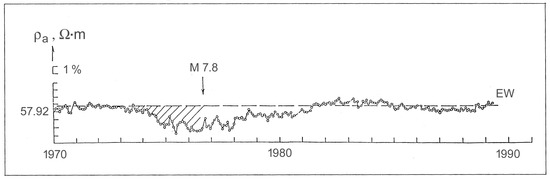
Figure 2.
Plot of ρa measured by the VES method from 1970 to 1990 at the Baodi station for the E-W line. Adapted from [32]. The arrow indicates the time of the Tangshan earthquake (28 July 1976, M 7.8). The dashed horizontal line is the level of stable behavior of apparent resistivity.
Prior to the Wenchuan earthquake in China (12 May 2008, M 8.0), the decrease in ρa values measured by the VES method was registered at several stations in the region (Figure 3). At the CDU station (35 km from the epicenter), the maximum decrease in ρa was 5.5%; at the JYO station (150 km), it was 1.1%; and at the GAZ station (331 km), it was 5.3%. At all stations, the decrease in ρa values occurred over a period of approximately two years before the earthquake [11].
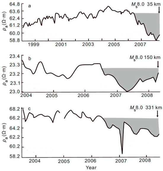
Figure 3.
Plots of ρa measured by the VES method at three monitoring stations in the region of the Wenchuan earthquake (12 May 2008, M 8.0). Adapted from [11]. (a) CDU station for N56° E component, (b) JYO station for N70° W component, (c) GAZ station for N30° E component.
The anomalies in Figure 3 were identified by a visual qualitative analysis of the behavior of the recorded parameters as compared to the background level in the previous period. It is well seen in Figure 3a,c. The anomaly in Figure 3b in 2007–2008 is very small (1.1%), but it can be considered a precursor to the accuracy of measurements (0.1–0.3%). A similar anomaly in 2005 is smaller (approximately 0.5%), barely exceeding the measurement error.
These examples of reliably detected ρa variations using the DC VES method show a typical behavior of this parameter before earthquakes. In most cases, a relatively smooth decrease in ρa values was observed, occurring over 2–2.5 years before the earthquakes. However, sometimes an increase in apparent resistivity occurs, and anomalies are observed at shorter times prior to earthquakes. The above examples of ρa anomalies based on significant experience in applying the VES method using a network of stations in China are described in numerous publications [11,16] and can be considered as reliably determined and associated with subsequent earthquakes.
Despite the fact that the VES method was used in China for many years to monitor ρa variations, its informative value is limited because of the single depth for a used current line size. Additionally, the observation system with fixed pillar-mounted lines of 1–3 km length occupies a large territory (Figure 1). Measured data are often subject to interference from non-seismic factors (rain, irrigation system operation, influence of metal pipelines) [11].
Recently, a new system has been developed in China for the observation of alternating electromagnetic fields in the frequency range of 0.1–300 Hz from a powerful radio transmitter with an operating range of up to 2000–3000 km. This system consists of two differently oriented transmitter lines mounted on power lines 80 km long (E-W direction) and 60 km long (N-S direction), two 500 kW transmitters, and 30 MT-AMT sounding monitoring stations [33]. In addition to the fields from the controlled source, natural electromagnetic fields in the frequency range of 0.001–1000 Hz are also measured. This system is designed, among other tasks, to record variations in ρa as earthquake precursors and is referred to as the Wireless Electromagnetic Method (WEM) in publications by Chinese authors [33].
We review now our experience in monitoring ρa variations using MT-AMT sounding methods. When conducting measurements, it is important to ensure sufficient sounding depth to exclude the influence of seasonal and meteorological factors. The optimal frequency range for monitoring ρa variations is 7–300 Hz, where measurements of the natural electromagnetic field are most reliable and provide high-quality data (errors of 0.5% in apparent resistivity and 0.5° in impedance phase). The lower limit of this range is near to the first Schumann resonance (8 Hz), and the upper limit is dictated by a need to ensure a sufficiently high level of natural electromagnetic field throughout the year.
It is not advisable to increase the depth of resistivity investigation by measuring at lower frequencies, as the locations of earthquake foci are often not optimal relative to the monitoring stations, making it difficult to detect anomalies related to changes in rock properties in the focal zones. Changes in rock resistivity in the focal zones can be significant, but registering these at monitoring sites is challenging.
Furthermore, our data indicate that in the frequency range of 1–6 Hz in a seismically quiet area (Leningrad region, Russia), significant (up to an order of magnitude) daily changes in ρa values were observed, while in the frequency range of 7–40 Hz, this parameter showed stable behavior (Figure 4). This is explained by the instability and changes in the polarization of the natural electromagnetic field in the magnetotelluric “dead band” (0.5–7 Hz), where the low-level and complicated behavior of the fields is observed [34]. Scatter in apparent resistivity and impedance phase values is observed when a fault is located near a measurement point and the direction of the field polarization is changed within a day.
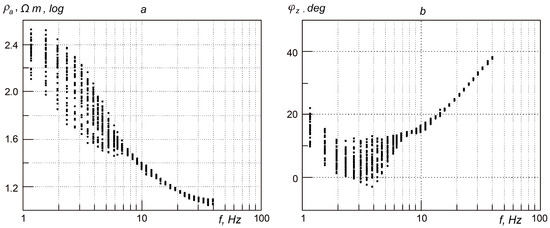
Figure 4.
AMT sounding curves of apparent resistivity (a) and impedance phase (b) in the frequency range of 1–40 Hz based on 34 one-hour measurements (Leningrad Region, Russia).
Conducting MT-AMT monitoring, it is advisable to process data measured at frequencies below 7 Hz by analysis of the behavior of the magnetic and electrotelluric field components. Data processing should differ from standard magnetotelluric approaches that aim at excluding signals with a non-stationary behavior, which may be earthquake precursors. Nevertheless, even without excluding non-stationary signals, data can be presented in the usual form for magnetotellurics (plots or pseudosections of apparent resistivity and impedance phase). It should also be borne in mind that variations in the magnetic and electrotelluric fields may be caused by nearby sources. In this case, source depth cannot be estimated from the plane wave model and skin-layer thickness.
According to modern views [17], most precursor anomalies are not generated in the focal zone of the future earthquake. The area over which precursor anomalies manifest themselves is much larger than the fault length in the focal zone. Therefore, when setting up networks for monitoring variations in apparent resistivity, it is advisable to focus on identifying active faults and searching for stress–strain sensitive zones to install the measurement equipment.
Selecting stress–strain sensitive zones includes analyzing the geological features of the territory, conducting field studies to investigate the geoelectric structure of preliminarily selected sites, and performing test monitoring sessions to assess the response to the medium tidal deformations. Our experience in studying ρa tidal variations has shown that stress–strain sensitive zones are characterized by heterogeneous structures and are usually located near faults. Tidal variations are observed when the thickness of overlying sediments is small and the investigation depth of the used sounding method allows the study of the bedrock. The most noticeable tidal variations in ρa were observed when the rocks have high resistivity and small moisture content [35]. Registration of tidal variations in apparent resistivity is a fruitful research area in its own right [19,36,37,38]. Conducting short monitoring sessions at pre-selected points helps assess the possibility of recording tidal effects in the ρa variations.
AMT sounding curves obtained at two sites on the Bishkek test site (Kyrgyzstan) are shown in Figure 5. Curves with index 1 correspond to the azimuth of the measuring array at 0°, with index 2—to 90°. The measuring array consists of a receiving line of the electric field and a magnetic antenna, located horizontally and mutually perpendicular. The direction of the electric line corresponds to the azimuth of the sounding curve. The Tash Bashat (I) and Uch Emchek (II) sites are located in different areas of the Bishkek test site.
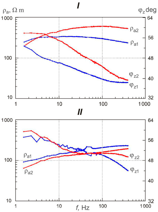
Figure 5.
AMT sounding curves in different areas of the Bishkek test site for the points Tash Bashat (I) and Uch Emchek (II) (Bishkek test site). Indices 1 and 2 correspond to directions 0° and 90°, respectively.
The behavior of the sounding curves characterizes the heterogeneity of the section at the Tash Bashat site. The curves at the Uch Emchek site indicate the homogeneity of rocks. Figure 6 shows plots of ρa2 compared to the calculated vertical tidal deformation of the Earth’s crust dH [38]. In the stress–strain sensitive point Tash Bashat, a close correlation between the plots of ρa2 and dH is observed, while in the non-sensitive point Uch Emchek there is no such correlation. Curves ρa1 for azimuth 0° show the similar behavior.
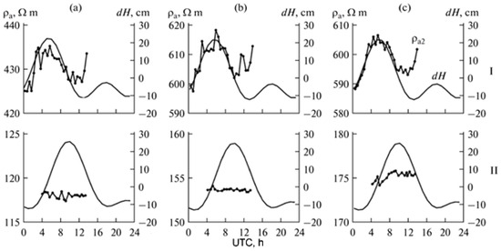
Figure 6.
Results of the test monitoring for the Tash Bashat (I) and Uch Emchek (II) sites (Bishkek test site) at different frequencies ((a)—7 Hz, (b)—70 Hz, (c)—175 Hz) for ρa2 at an azimuth of 90° and calculated curves of vertical tidal deformation dH. The left vertical axes show values of apparent resistivity, the right vertical axes—values of vertical tidal deformation, and the horizontal axes—UTC time.
We used the ACF-4M system, intended for magnetotelluric–audiomagnetotelluric soundings in the frequency range of 0.1–1000 Hz, in the Leningrad region and on the Bishkek test site [12]. The system includes a digital recorder, four synchronous channels and a 24-bit analog-to-digital converter per channel for measuring horizontal components of the electric (Ex, Ey) and magnetic (Hx, Hy) fields, a preamplifier of electric channels, two symmetrical receiving electric lines, and two magnetic antennas (induction sensors). ACF-4M was used both for monitoring with the software-controlled measurement process and at a preliminary stage for the study of the geoelectric structure of earthquake-prone areas and selection of stress–strain sensitive places for the installation of monitoring stations. Standard magnetotelluric procedures were used at the data registration and processing. Spectral analysis of the registered time series was carried out, and spectral characteristics of measured field components as well as the determination of impedance amplitude (apparent resistivity ρa) and impedance phase φz were calculated. Auto spectra of horizontal and mutually orthogonal electric and magnetic field components have been used to derive the sounding curves.
3. Monitoring of Electromagnetic Emission
We consider now the AMT monitoring data obtained in China using the new WEM monitoring system and data of measuring natural electromagnetic fields. Figure 7 shows the position of the Yangbi earthquake epicenter and the Dali monitoring station, located 32 km from the earthquake epicenter [39]. The Yangbi earthquake occurred on 27 March 2017, with a magnitude of M 5.1. Also, the location of the Yunlong (18 May 2016, M 5.0) earthquake epicenter and large earthquakes are shown.
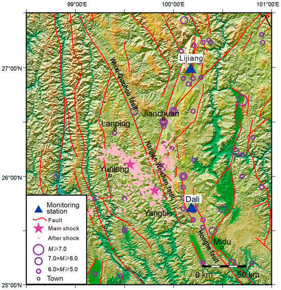
Figure 7.
Locations of the Yangbi (27 March 2017, M 5.1) and Yunlong (18 May 2016, M 5.0) earthquake epicenters and the Dali and Lijiang monitoring stations. Adapted from [39]. Occurring in the past, large earthquakes are also shown in the map. Double circles represent earthquakes of different magnitudes in the same location.
The plots of apparent resistivity and impedance phase from the monitoring data at a frequency of 74 Hz are shown in Figure 8 [33]. These plots exhibit a pulsed behavior of apparent resistivity and phase, taking maximal and minimal values 15 days before the earthquake and both decreasing to background levels 3 days before the event. The relative value of ρa anomalies (over 100%) significantly exceeds the previously reported values for DC measurements using the VES method (a few percent). Additionally, the behavior of the ρa plots differs, the latter being smooth for ρa measured with the VES method and pulsed for ρa measured with the AMT method.
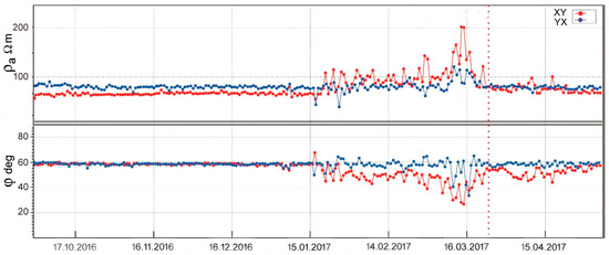
Figure 8.
Plots of apparent resistivity (ρa) and impedance phase (φ) at a frequency of 74 Hz, obtained from measurements at the Dali station from 1 October 2016, to 30 April 2017, before and after the Yangbi earthquake (27 March 2017, M 5.1). Adapted from [33]. The vertical dotted line indicates the time of the earthquake. The labels XY and YX correspond to the N-S and E-W directions, respectively. Horizontal axis—dates.
The salient features of the monitoring data presented in Figure 8 suggest that they should be considered as a manifestation of electromagnetic emission in the ELF range. Chinese experts consider a fault in the earthquake foci as a source of electromagnetic emission for the Yangbi earthquake (2017) and the Wenchuan earthquake (12 May 2008, M 8.0) [39,40]. Specifically, for interpreting the anomalous signal with an amplitude of 1.3 mV/m recorded at the Hebei Gaobeidian station, located 1440 km from the Wenchuan earthquake epicenter, Chinese authors assumed that the source of the anomaly in the focal zone could be approximated by an electric dipole (a linear horizontal current of 108 A, 150 km long, with a characteristic frequency of about 1 Hz) [40]. A similar interpretation of the signal source for the data obtained at the Dali station (Figure 8) indicated that the electric dipole in the focal zone of the Yangbi earthquake (2017) should have a dipole moment of around (2–3)∙109 A·m [39].
Worth noting that the presumed electric currents in these models should generate large magnetic fields. It can be shown that for the current of 108 A [40], the magnetic disturbances before the Wenchuan earthquake should have exceeded the Earth’s magnetic field over the entire distance from the epicenter to the observation point.
In our opinion, the sources of these anomalies are located closer to the monitoring sites compared to the distance of 32 km from the Yangbi earthquake epicenter to the Dali station. A more likely source of the anomalies before the Yangbi earthquake (2017), as shown in Figure 8, would be an active fault (or faults) located near the Dali station (Figure 7). The positive anomalies in ρa before the earthquake indicate a relatively short distance to the source, as would be expected from the behavior of this parameter in the near-field zone of the source. An increase in ρa in the near-field zone of a source approximated by an electric dipole is noted in [41].
Additionally, the higher values of ρa for the XY setup (receiving line direction N-S) compared to the YX setup (direction E-W) indicate that the faults oriented N-S extend latitudinally relative to the Dali station, as confirmed by Figure 7. It is known that the sensitivity of the E-polarized field to objects located to the side of the measuring electric line is higher than that of the H-polarized field [42]. The presence of submeridional active faults near the Dali station is indicated by the chain of epicenters of seismic events with magnitudes M5–M6 along these faults (Figure 7). The behavior of the ρa plots before the Yunlong earthquake (sign and amplitude of anomaly, duration) is similar to the case of the Yangbi earthquake [39].
Let us consider the monitoring data from January 2021 to April 2022 obtained at the Lijiang station (the location of the station is shown in Figure 7). Plots of apparent resistivity and impedance phase at frequencies of 3.9 Hz and 0.9 Hz are presented in Figure 9 [43]. During this period, there were a series of shocks with magnitudes up to M 6.5 in Yangbi County (2021) and up to M 5.5 in Ninglang County (2022). The series of shocks in Yangbi County occurred 35 km south of the previously discussed Yangbi earthquake (2017) (Figure 7). The epicenter of the Yangbi earthquake series (2021) was 170 km south from the Lijiang station. The epicenter of the Ninglang earthquake series was 88 km north of the Lijiang station (not shown in Figure 7).
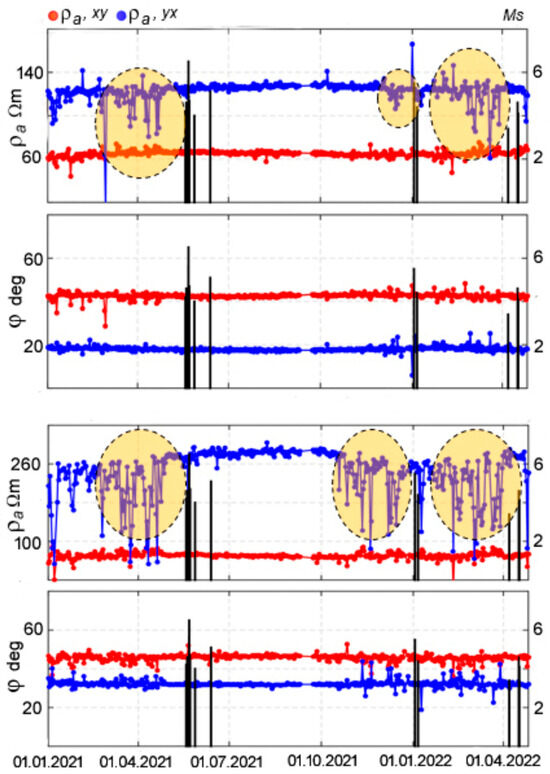
Figure 9.
Plots of apparent resistivity (ρa) and impedance phase (φ) at frequencies of 3.9 Hz (top) and 0.9 Hz (bottom) obtained from measurements at the Lijiang station from 1 January 2021 to 14 April 2022. Adapted from [43]. The series of Yangbi earthquakes (2021) are shownon the left, and the Ninglang earthquakes are shown on the right. Anomalies of apparent resistivity are shown by circles. The labels ρa(xy) and ρa(yx) correspond to the plots of apparent resistivity in the N-S and E-W directions, respectively (the same applies to the impedance phase). Horizontal axes—dates, Ms—magnitude of earthquakes.
The plots of ρa exhibit a pulsed behavior, which can be considered a manifestation of electromagnetic emission. Significant decreases in ρa values were observed before the two series of earthquakes. The relative values of ρa anomalies for the YX direction (receiver line direction E-W) in this case are substantially larger (more than 100%) than the characteristic anomalies for DC measurements using the VES method (a few percent). More pronounced anomalies are observed at the lower frequency of 0.9 Hz compared to 3.9 Hz. Note that immediately before the series of Yangbi (2021) and Wenchuan earthquakes, the ρa values returned to background levels.
Ji Tang et al. [43] attribute the registered ρa anomalies to a sub-latitudinal fault located close to the Lijiang monitoring station. In our opinion, this interpretation of the obtained data is correct, unlike the previously discussed examples for the Yangbi (2017) and Wenchuan earthquakes, which were obtained at the Dali monitoring station. However, the estimation of the possible depth of the source of these anomalies at 5–15 km, as given in [43], is questionable. As noted previously, the depth of a source located close to the monitoring station cannot be estimated using the conventional magnetotelluric approach based on the skin-layer thickness.
The sub-latitudinal fault south of the Lijiang monitoring station is not shown in Figure 7. However, out of four seismic events with magnitudes of M 5-6 near the Lijiang station, three form a sub-latitudinal chain. An additional indication of the presence of a sub-latitudinal fault is the higher anomalous values of ρa for the YX direction (E-W), corresponding to the E-polarized field, which has higher sensitivity to objects located to the side of the measuring electric line compared to the H-polarized field.
A possible explanation for the negative sign of the E-polarized field ρa anomalies for the Yangbi (2021) and Wenchuan earthquakes recorded at the Lijiang station, as compared to the positive ρa anomalies of the E- and H-polarized fields for the Yangbi (2017) earthquake recorded at the Dali station, may be as follows. The active fault near the Dali station is located relatively close, and the station is in the near-field zone of the source where a significant increase in ρa values is observed. The active fault near the Lijiang station is located farther away, and the station is in the transition zone of the source where no increase in ρa values is observed. In this case, the measurement data for the E-polarized field shows the influence of the conductive fault. For the H-polarized field, which has lower sensitivity to horizontally distant objects, anomalies are virtually absent.
An additional indication of the influence of the sub-latitudinal fault on the measurement data at the Lijiang station is the difference in the anomalies at frequencies of 0.9 Hz and 3.9 Hz (Figure 9). When estimating the possible distance of the station from the fault, it should be borne in mind that the horizontal skin depth for the E-polarized field is approximately three times larger than the vertical skin depth. At the frequency of 0.9 Hz, the thickness of the vertical skin depth is greater than at 3.9 Hz, and accordingly the size of the horizontal skin depth is larger. Therefore, the anomalous changes in ρa for the Yangbi (2021) and Wenchuan earthquakes are most likely associated with a sub-latitudinal fault located south of the Lijiang monitoring station.
The salient features of anomalies—earthquake precursors discussed in this section—are based on the analysis of several examples obtained from recent observations using the magnetotelluric sounding method. It should be borne in mind that the appearance of anomalies can be more diverse depending on the geological features of the sites where monitoring stations are located. Whereas the experience of using magnetotelluric monitoring is more limited than the VES monitoring described above, the examples of anomalies (Figure 8 and Figure 9) are quite convincing and can be considered to be related to subsequent earthquakes with a high degree of probability.
When conducting magnetotelluric monitoring, it should be borne in mind that industrial interference and nearby thunderstorms have a significant impact on the quality of the data obtained. With a high level of industrial noise or thunderstorm activity, it is difficult to obtain high-quality data and, accordingly, reliable conclusions about whether or not the recorded anomalies are precursors of earthquakes. In addition, electromagnetic emission anomalies may manifest themselves not explicitly as contrasting pulses significantly exceeding background values but as hidden anomalies in time series of observed parameters. The identification of the latter requires further development of approaches and methods for data processing. Qualitative data analysis is not sufficient for reliable interpretation of magnetotelluric monitoring results. It is necessary to conduct modeling and use quantitative methods to estimate the parameters of anomalies, which is the subject of further work.
Naturally, the considered method alone cannot reliably solve the problem of earthquake prediction. The data obtained should be interpreted taking into account data from other methods of monitoring seismic activity—seismic, geodeformation, geochemical, geothermal, hydrogeological, etc. To determine the place of magnetotelluric monitoring in early warning systems, it is necessary to conduct research in this area.
The possible nature of electromagnetic emission in fault zones, including the presented examples from the Dali and Lijiang monitoring stations, is beyond the scope of this paper.
4. Conclusions
We discuss the performance of the VES monitoring system in China for the registration of variations in apparent resistivity as an earthquake precursor, along with observations before the Tangshan (1976) and Wenchuan (2008) earthquakes. Typically, the decreases in ρa values were observed, which were relatively smooth and occurred over a period of 2–2.5 years before the earthquakes.
We further discuss the technique for recording variations in apparent resistivity and electromagnetic emission based on measurements of natural electromagnetic fields during magnetotelluric monitoring of earthquake precursors in the ULF-ELF ranges. Standard data processing for the studying of variations in rock resistivity is advisable in the frequency range of 7–300 Hz, where measurements of natural electromagnetic fields are the most reliable and yield high-quality data. The use of measurement data at frequencies below 7 Hz should be based on the analysis of variations in the magnetic and electrotelluric field components.
The authors’ experience in selecting stress–strain sensitive zones for installing measurement equipment is outlined. The research roadmap includes analyzing the geological features of the territory, conducting field studies to investigate the geoelectric structure of preliminarily selected sites, and performing test-monitoring sessions to assess the electromagnetic response of the medium to tidal deformations.
Information is provided about the new WEM monitoring system in China based on recording electromagnetic fields from a powerful radio transmitter in the frequency range of 0.1–300 Hz and natural electromagnetic fields in the frequency range of 0.001–1000 Hz. The results obtained by Chinese researchers using the WEM system during magnetotelluric monitoring based on measurements of natural electromagnetic fields are discussed.
The analysis of monitoring data obtained at the Dali station at a frequency of 74 Hz before the Yangbi earthquake (2017) shows that the plots of apparent resistivity and impedance phase have a pulsed behavior and should be considered as manifestations of electromagnetic emission. Relative anomalies of ρa (over 100%) significantly exceed the relative variations in DC measurements using a VES method (a few percent). In this case, a more likely source of electromagnetic emission is an active fault (or faults) located close to the monitoring station, rather than the earthquake’s focal zone itself. The increase in ρa values before the earthquake indicates a nearby source, as suggested by the behavior of this parameter in the near-field zone of the source. The ρa values for the N-S direction (E-polarized field) exceed those for the E-W direction (H-polarized field). It can be explained by the higher sensitivity of the E-polarized field to objects located to the side of the receiving electric line. This indicates the presence of a fault oriented N-S relative to the Dali station. The presence of sub-meridional active faults around the Dali station is also indicated by the chain of epicenters of seismic events along the N-S direction.
Unlike the positive anomalies for the Yangbi earthquake (2017), negative anomalies of ρa were recorded at the Lijiang station in other cases, with a pulsed behavior corresponding to manifestations of electromagnetic emission before the Yangbi (2021) and Ninglang (2022) earthquake series. In this case, Chinese experts consider a sub-latitudinal fault located close to the Lijiang station as the source. It is confirmed by the chain of seismic events along the E-W direction. The ρa values in the E-W direction correspond to the E-polarized field, which has higher sensitivity to objects located to the side of the receiving electric line, confirming the presence of a sub-latitudinal fault.
The different signs of ρa anomalies before the Yangbi (2017) earthquake and the Yangbi (2021) and Ninglang (2022) earthquake series can be explained by that in the first case, the active fault near the Dali station is located relatively close, and the station is in the near-field zone of the source where an increase in ρa values is observed. The active fault near the Lijiang station is located farther away, and the station is located in the transition zone of the source where no significant increase in ρa values is observed, and this fault appears as a conductive object in the measurement data.
Chinese experts suggest that faults in the focal zones of the Wenchuan (2008) and Yangbi (2017) earthquakes should be viewed as sources of electromagnetic emission. However, this requires an unrealistically large current in the source (108 A for the Wenchuan earthquake) and dipole moment of the source ((2–3)∙109 A·m for the Yangbi earthquake). The likely sources of anomalies in the ULF-ELF ranges before the Yangbi (2017), Yangbi (2021), and Ninglang (2022) earthquakes in China are active faults located close to the monitoring stations. Their influence manifests itself during the preparation periods of earthquakes due to tectonic activation of the region. For powerful earthquakes like the Wenchuan one, the activation region can be very large, several thousand kilometers. Accordingly, precursor anomalies can occur at big distances from the earthquake epicenters on monitoring stations located at active faults.
Measurements of natural electromagnetic fields show that variations in apparent resistivity have a pulsed behavior and are manifestations of electromagnetic emission. Different signs of anomalies can be explained by the varying distances between the monitoring stations and the faults corresponding to the near-field or transition zones of the sources. However, estimating possible depths of precursor anomalies sources, making use of generally accepted procedures of magnetotellurics, such as the plane wave model and skin-layer thickness, may yield inadequate results when analyzing records of electromagnetic emissions from nearby sources.
The approaches to the analysis of magnetotelluric monitoring data in a wide frequency range proposed in this study require further development and verification based on observations at prognostic test sites, taking into account the influence of industrial noise, space weather and thunderstorm activity. It is necessary to obtain additional data on the manifestation of tidal variations in the recorded values of apparent resistivity and impedance phase, as well as in the parameters of electromagnetic emission. It should be borne in mind that electromagnetic emission can manifest itself both as pulse anomalies in the graphs of the parameters used and as hidden anomalies in the time series of the components of the electrotelluric and magnetic fields, the latter requiring the development of special data processing methods.
Author Contributions
Conceptualization, A.K.S.; methodology, A.K.S. and V.S.; software, A.A.S.; validation, V.P.; formal analysis, V.S.; investigation, A.K.S., A.A.S. and S.A.; resources, M.D.; data curation, A.A.S., D.Z. and S.A.; writing—original draft preparation, A.K.S.; writing—review and editing, V.S., V.P., N.B., M.D. and S.A.; visualization, N.B. and D.Z.; project administration, N.B. All authors have read and agreed to the published version of the manuscript.
Funding
This work was supported by the Russian Science Foundation (project 25-47-01004) and the Ministry of Science and Technology of India (project TPN/120765).
Data Availability Statement
The original contributions presented in this study are included in the article. Further inquiries can be directed to the corresponding author.
Acknowledgments
The studies in Russia and Kyrgyzstan were performed with the facilities provided by the Research Park of St. Petersburg State University, «Center for Geo-Environmental Research and Modeling (GEOMODEL)».
Conflicts of Interest
The authors declare no conflicts of interest.
Abbreviations
The following abbreviations are used in this manuscript:
| ULF | Ultra-low frequency |
| ELF | Extremely low frequency |
| MT | Magnetotelluric |
| AMT | Audiomagnetotelluric |
| DC | Direct current |
| VES | Vertical electrical sounding |
| WEM | Wireless electromagnetic method |
References
- Uyeda, S.; Nagao, T.; Kamogawa, M. Short-term earthquake prediction: Current status of seismo-electromagnetics. Tectonophysics 2009, 470, 205–213. [Google Scholar] [CrossRef]
- Fraser-Smith, A.C. The ultra-low frequency magnetic fields associated with and preceding earthquakes. In Electromagnetic Phenomena Associated with Earthquakes; Hayakawa, M., Ed.; Transworld Research Network: Trivandrum, India, 2009; pp. 1–20. [Google Scholar]
- Kopytenko, Y.; Ismagilov, V.; Nikitina, L. Study of local anomalies of ULF magnetic disturbances before strong earthquakes and magnetic fields induced tsunami. In Electromagnetic Phenomena Associated with Earthquakes; Hayakawa, M., Ed.; Transworld Research Network: Trivandrum, India, 2009; pp. 20–40. [Google Scholar]
- Surkov, V.; Hayakawa, M. Ultra and Extremely Low Frequency Electromagnetic Fields; Springer: Tokyo, Japan, 2014; 486p. [Google Scholar]
- Park, S.K.; Johnston, M.J.S.; Madden, T.R.; Morgan, F.D.; Morrison, H.F. Electromagnetic precursors to earthquakes in the ULF band: A review of observations and mechanism. Rev. Geophys. 1993, 31, 117–132. [Google Scholar] [CrossRef]
- Johnston, M.J.S. Review of electric and magnetic fields accompanying seismic and volcanic activity. Surv. Geophys. 1997, 18, 441–475. [Google Scholar] [CrossRef]
- Surkov, V.; Pilipenko, V. The physics of pre-seismic electromagnetic ULF signals. In Atmospheric and Ionospheric Electromagnetic Phenomena Associated with Earthquakes; Hayakawa, M., Ed.; Terra Scientific Publishing Company: Tokyo, Japan, 1999; pp. 357–370. [Google Scholar]
- Hattori, K. ULF Geomagnetic Changes Associated with Large Earthquakes. Terr. Atmos. Ocean. Sci. 2004, 15, 329–360. [Google Scholar] [CrossRef]
- Thomas, J.; Love, J.; Johnston, M.; Yumoto, K. On the reported magnetic precursor of the 1993 Guam earthquake. Geophys. Res. Lett. 2009, 36, 1–5. [Google Scholar] [CrossRef]
- Masci, F.; Thomas, J. Are there any new findings in the research for ULF magnetic precursors to earthquakes? J. Geophys. Res. Space Phys. 2015, 120, 10289–10304. [Google Scholar] [CrossRef]
- Zhao, G.; Zhang, X.; Cai, J.; Zhan, Y.; Ma, Q.; Tang, J.; Du, X.; Han, B.; Wang, L.; Chen, X.; et al. A review of seismo-electromagnetic research in China. Sci. China Earth Sci. 2022, 65, 1229–1246. [Google Scholar] [CrossRef]
- Saraev, A.K.; Antaschuk, K.M.; Simakov, A.E.; Bakirov, K.B. Multiparameter Monitoring of Electromagnetic Earthquake Precursors in the Frequency Range 0.1 Hz–1 MHz. Seism. Instrum. 2014, 50, 52–66. [Google Scholar] [CrossRef]
- Barsukov, O.M.; Sorokin, O.N. Variations in apparent resistivity of rocks in the seismically active Garm region. Izv. Phys. Solid Earth 1974, 9, 685–687. [Google Scholar]
- Mogi, K. Earthquake Prediction; Academic Press: Tokyo, Japan, 1985; 382p. [Google Scholar]
- Sobolev, G.A. Fundamentals of Earthquake Prediction; Nauka: Moscow, Russia, 1993; 314p. (In Russian) [Google Scholar]
- Lu, J.; Qian, F.; Zhao, Y. Sensitivity analysis of the Schlumberger monitoring array: Application to changes of resistivity prior to the 1976 earthquake in Tangshan, China. Tectonophysics 1999, 307, 397–405. [Google Scholar] [CrossRef]
- Sobolev, G.A.; Ponomarev, A.V. Earthquake Physics and Precursors; Nauka: Moscow, Russia, 2003; 270p. (In Russian) [Google Scholar]
- Gere, J.M.; Shah, H.C. Terra Non Firma. Understanding and Preparing for Earthquakes; W.H. Freeman and Company: Madison, NY, USA, 1984; 203p. [Google Scholar]
- Rybin, A.K.; Bataleva, E.A.; Aleksandrov, P.N.; Nepeina, K.S. Electromagnetic Studies of Present Geodynamic Processes in the Lithospheres of the Regions of Intracontinental Orogeny: The Tien Shan Example. Izv. Phys. Solid Earth 2022, 58, 690–705. [Google Scholar] [CrossRef]
- Seminsky, I.K.; Pospeev, A.V. Reflection of Strong 2020–2021 Baikal Rift Earthquakes in the Earth’s Magnetotelluric Field Observation Data. Izv. Phys. Solid Earth 2022, 58, 484–492. [Google Scholar] [CrossRef]
- Kopytenko, Y.A.; Matiashvili, T.G.; Voronov, P.M.; Kopytenko, E.A.; Molchanov, O.A. Detection of ULF emissions connected with the Spitak earthquake and its aftershock activity, based on geomagnetic pulsation data at Dusheti and Vardzia observations. Phys. Earth Planet. Inter. 1993, 77, 85–95. [Google Scholar] [CrossRef]
- Hayakawa, M.; Kawate, R.; Molchanov, O.A.; Yumoto, K. Results of ultra-low frequency magnetic field measurements during the Guam earthquake of 8 August 1993. Geophys. Res. Lett. 1996, 23, 241–244. [Google Scholar] [CrossRef]
- Hattoi, K.; Akinaga, Y.; Hayakawa, M.; Yumoto, K.; Nagao, T.; Uyeda, S. ULF magnetic anomaly preceding the 1997 Kagoshima Earthquakes. In Seismo Electromagnetics; TERRAPUB: Tokyo, Japan, 2002; pp. 19–28. [Google Scholar]
- Hobara, Y.; Koons, H.C.; Roeder, J.L.; Yamaguchi, H.; Hayakawa, M. New ULF/ELF observation in Seikoshi, Izu, Japan, and the precursory signal in relation with recent large seismic events near Izu. In Seismo Electromagnetics: Lithosphere-Atmosphere-Ionosphere Coupling; Hayakawa, M., Molchanov, O.A., Eds.; TERRAPUB: Tokyo, Japan, 2002; pp. 41–44. [Google Scholar] [CrossRef]
- Sobolev, G.A. Prospects for operational earthquake forecasting based on electrotelluric observations. Harbingers Earthq. 1973, 5498, 172–185. (In Russian) [Google Scholar]
- Varotsos, P.; Alexopulos, K. Physical properties of the variations of the electric fields of the Earth proceeding earthquakes. Tectonophysics 1984, 110, 73–125. [Google Scholar] [CrossRef]
- Gokhberg, M.B.; Morgunov, V.A.; Pokhotelov, O.A. Seismoelectromagnetic Phenomena; Nauka: Moscow, Russia, 1988; 174p. (In Russian) [Google Scholar]
- Eftaxias, K.; Kapiris, P.; Polygiannakis, J.; Bogris, N.; Kopanas, J.; Antonopoulos, G.; Peratzakis, A.; Hadjicontis, V. Signature of pending earthquake from electromagnetic anomalies. Geophys. Res. Lett. 2001, 28, 3321–3324. [Google Scholar] [CrossRef]
- Nagao, T.; Enomoto, Y.; Fujinawa, Y.; Hata, M.; Hayakawa, M.; Huang, Q.; Izutsu, J.; Kushida, Y.; Maeda, K.; Oike, K.; et al. Electromagnetic anomalies associated with 1995 Kobe earthquake. J. Geodyn. 2002, 33, 401–411. [Google Scholar] [CrossRef]
- Hayakawa, M. Electromagnetic Phenomena Associated with Earthquakes; Transworld Research Network: Trivandrum, India, 2009; 279p. [Google Scholar]
- Xie, T.; Xue, Y.; Ye, Q.; Lu, J. Anisotropic change in apparent resistivity before earthquakes of MS ≥ 7.0 in China mainland. Geomat. Nat. Hazards Risk 2022, 13, 1207–1228. [Google Scholar] [CrossRef]
- Qian, F.; Zhao, B.; Lu, F. Georesistivity precursors to the Tangshan earthquake of 1976. Ann. Geophys. 1997, 40, 251–260. [Google Scholar] [CrossRef]
- Lu, J.; Zhuo, X.; Liu, Y.; Zhao, G.; Di, Q. The Extremely Low Frequency Engineering Project for Underground Exploration. Engineering 2022, 10, 13–20. [Google Scholar] [CrossRef]
- Simpson, F.; Bahr, K. Practical Magnetotellurics; Cambridge University Press: Singapore, 2005; 254p. [Google Scholar]
- Saraev, A.K.; Pertel, M.I.; Malkin, Z.M. Monitoring of tidal variations of apparent resistivity. Geol. Acta 2010, 8, 5–13. [Google Scholar] [CrossRef]
- Al’tgauzen, N.M.; Barsukov, O.M. On time variations of electrical conductivity. In Physical Grounds of Searches for Earthquake Prediction Methods; Nauka: Moscow, Russia, 1970; pp. 104–110. (In Russian) [Google Scholar]
- Avagimov, A.A.; Ataev, A.I.; Ataev, S.A. Connection of abnormal changes in the electrical resistivity of rocks in the fault zone with tidal deformations of the Earth’s crust. Izv. Akad. Nauk Turkm. Ser. Fiz.-Mat. Tekh. Khim. Geol. Nauk. 1988, 5, 50–52. (In Russian) [Google Scholar]
- Saraev, A.K.; Pertel, M.I.; Malkin, Z.M. Manifestation of deformations of the Earth’s crust caused by tides and changes in the impedance of the electromagnetic field of the ELF radio station. Probl. Geophys. 1998, 35, 136–147. (In Russian) [Google Scholar]
- Han, B.; Hu, W.; Zhao, G.; Tang, J. Identifying and localizing of seismogenic electromagnetic anomalies from data observed by permanent MT stations. Sci. China Earth Sci. 2024, 67, 1698–1713. [Google Scholar] [CrossRef]
- Li, M.; Tan, H.; Cao, M. Ionospheric influence on the seismo-telluric current related to electromagnetic signals observed before the Wenchuan MS 8.0 earthquake. Solid Earth 2016, 7, 1405–1415. [Google Scholar] [CrossRef]
- Fan, Y.; Hu, W.; Han, B.; Tang, J.; Wang, X.; Ye, Q. Characteristic identification of seismogenic electromagnetic anomalies based on station electromagnetic impedance. Front. Earth Sci. 2023, 11, 1110056. [Google Scholar] [CrossRef]
- Saraev, A.K.; Antaschuk, K.M.; Eremin, I.S. Audio-frequency magnetotelluric surveys with non-grounded lines for imaging the resistivity structure of the Rybachiy Peninsula (Murmansk region). Earth’s Cryosph. 2018, 22, 57–66. [Google Scholar]
- Tang, J.; Wang, L.; Han, B.; Dong, Z.; Yang, S. Study on the relationship between pre-earthquake variation of resistivity and regional stress field. In Proceedings of the Abstract, 26th EM Induction Workshop, Beppu, Japan, 7–13 September 2024; pp. 1–3. [Google Scholar]
Disclaimer/Publisher’s Note: The statements, opinions and data contained in all publications are solely those of the individual author(s) and contributor(s) and not of MDPI and/or the editor(s). MDPI and/or the editor(s) disclaim responsibility for any injury to people or property resulting from any ideas, methods, instructions or products referred to in the content. |
© 2025 by the authors. Licensee MDPI, Basel, Switzerland. This article is an open access article distributed under the terms and conditions of the Creative Commons Attribution (CC BY) license (https://creativecommons.org/licenses/by/4.0/).