Abstract
This paper presents a Python-based simulation technique that can be used to predict the behavior of switch-mode non-isolated (SMNI) DC-DC converters operating in closed loop. The proposed technique can be implemented in an open-source numerical computation software, such as Scilab, Octave or Python, which makes it versatile and portable. The software that will be used to implement the proposed technique is Python, since it is an open-source programming language, unlike MATLAB, which is one of most-used programming and numeric computing platforms to simulate this type of system. The proposed technique requires the discretization of the equations that govern the open-loop operation of the converter, as well as the discretization of the transfer function of the controller. To simplify the implementation of the simulation technique, the code must be subdivided into different modules, which together form a package. The converter under analysis will be a buck converter operating in CCM. The proposed technique can be extended to any other SMNI DC-DC converter. The validation of the proposed technique will be carried out by comparing it with the results obtained in LTspice.
1. Introduction
Power electronics is a branch of electronics whose purpose is to develop systems that convert power from one form (source) to another form (load), as efficiently as possible. The aforementioned systems can be designed to operate in the power range from few W to MW, and can be found in home appliances, electric drives, renewable energy applications, electric trains, electric and hybrid cars and buses, industrial drives, and wireless power charging (smartphones and cars) [1], among others.
The aforementioned applications require different types of systems, which can be subdivided into four categories: AC/AC, AC/DC, DC/DC and DC/AC. In turn, each of these systems may have multiple circuits which can be used for a particular application. Usually, an application is composed of several stages which may contain different categories of power converters.
This paper focuses on the DC/DC converters, which are widely used in computer power supplies (ATX power supply) and servers, as well as in different types of charges and adapters (smartphones, tablet, laptops, etc.) that are used in our daily life.
The design of power converters requires the understanding of the working principle of the circuits and their analysis, but also the use of simulation tools.
One of the most commonly used tools to simulate power converters [2,3,4,5,6,7,8,9,10,11], as well as its components [12], is MATLAB/Simulink. The simplicity of the design of power converters, the high level of precision and user-friendly graphical interface makes this software very appealing [13,14], especially with regard to Simulink as it allows for Model-Based Design (MBD). MATLAB/Simulink plays a key role in carrying out research tasks [2,3,4,5,6,7,8,9,10,11,12,13,14].
One of the major disadvantages of MATLAB is the fact that it is a proprietary programming language unlike Python. As the algorithms implemented in MATLAB are proprietary, it is not possible to access their code. This particularity can significantly limit the implementation of control methods, as well as the development of fault diagnosis techniques [15].
Although Python does not allow MBD as MATLAB does, it has computational power and tools that make it possible to simulate DC/DC converters, as will be demonstrated in this paper.
On the other hand, the use of Python is clearly advantageous when applying machine-learning algorithms. Python has many libraries and packages for old and new machine-learning models, being widely used in this context in both industry and academia [16,17]. MATLAB has also some machine-learning algorithms that can provide immediate visual feedback, however these algorithms are proprietary.
The use of machine-learning algorithms can be very useful in converter design, in particular with regard to the control methods [7,8,9], and in the development of fault diagnosis techniques [18,19,20,21], making the proposed technique particularly suitable in these contexts.
The rest of this article is organized as follows. Section 2 describes the application of the proposed technique to a converter operating in open loop. Section 3 presents the converter design process and Section 4 shows how to apply the proposed technique to a converter operating in closed loop. Section 5 shows the feasibility of the proposed technique through its comparison with LTspice. Finally, Section 6 presents the conclusions.
2. Simulation of the Open-Loop Operation
The buck converter is suitable for IC (Integrated Circuit) power supplies, such as those used in Internet of Things (IoT) [22], rural DC micro-grids [23], fast charging of electric vehicles (EV) [24], solar photovoltaic (PV) systems [25].
Figure 1 shows the electric circuit of a buck converter.
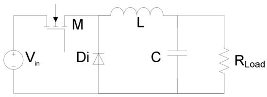
Figure 1.
Buck converter circuit.
The buck converter (Figure 1) is composed of two semiconductors—a diode (Di) and a transistor (M), and two reactive elements—an inductor (L), and a capacitor (C). It can operate in two conduction modes: continuous conduction (CCM) and discontinuous conduction mode (DCM). The DCM will rise if the inductor current reaches a zero value.
In this paper it will be considered that the buck converter is operating in CCM, thus, only two stages will be analyzed: the conduction state and the non-conduction state.
2.1. Stage I—Conduction State
During the conduction stage, the transistor M turns on and the diode Di is reverse-biased, so the current will pass through the inductor L which stores energy in the form of a magnetic field; simultaneously, the capacitor C is charged (Figure 2).
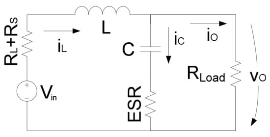
Figure 2.
Buck converter circuit during the conduction state.
Through the analysis of the previous circuit, it is possible to write the following equations:
2.2. Stage II—Non-Conduction State
During the non-conduction state, the transistor is turned off, which forces the current to free wheel around the path consisting of L, C and Di (Figure 3).
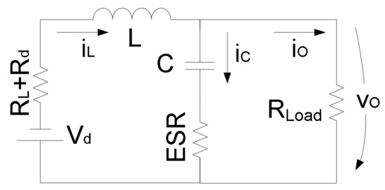
Figure 3.
Buck converter circuit during the non-conduction state.
Through the analysis of the previous circuit, it is possible to write the following equations:
where Vin, RL, L, RS, Vd, Rd, C, ESR, RLoad, iL, iC, iO, vO and vC, represent the input voltage, inductor resistance, inductor inductance, drain-source resistance, diode forward voltage drop, diode internal resistance, capacitor capacitance, capacitor internal resistance, load resistance, inductor current, capacitor current, load current, output voltage and output voltage component due exclusively to C, respectively.
Finally, the following set of equations can be presented, that apply to both states.
2.3. Open-Loop Simulation
As previously mentioned, the simulation technique will be implemented in Python. Thus, it is important to briefly introduce the main tools that will be used in this context.
Python is a high-level, general-purpose programming language that can be used to develop numerical computation applications, such as simulation of physical systems. For this purpose, it is essential to use some Python libraries. The most important ones, in this context, are NumPy and Matplotlib. The Numerical Python package (Numpy) is used to manipulate arrays and matrices, and the Matplotlib package is used for plotting.
To simplify the implementation of the simulation technique, the code must be subdivided into different modules, which together form a package. The first module must contain two functions that compute iL, iC, vC and vO values during the conduction state (Figure 4) and during the non-conducting state (Figure 5).
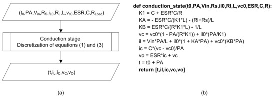
Figure 4.
Function that models the behavior of the converter during the on state: (a) Algorithm and (b) Python code.
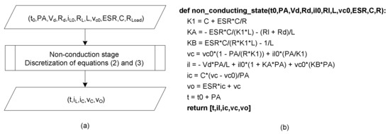
Figure 5.
Function that models the behavior of the converter during the off state: (a) Algorithm and (b) Python code.
Thus, after discretizing Equation (1), it is possible to construct a function that describes the operation of the converter during the conduction state (Figure 4). This function must receive as input arguments the initial time, t0, the sampling period, PA, the characteristics of the converter (Vin, RS, L, ESR, C and RLoad) and the initial conditions (the inductor current, iL0, and capacitor voltage, vC0, at the initial time).
Following this, the same procedure must be applied for the non-conduction state, in order to obtain the non-conducting state function (Figure 5).
The previous function (Figure 5) takes practically the same input arguments as the function in Figure 4. The difference between the two functions is related to the input arguments, as can be seen by comparing Equations (1) and (2).
After creating the module which reproduces the conduction and non-conducting states, it is necessary to create a new one: the module that will be responsible for generating the output signal of the Pulse Width Modulator (PWM). This module will be composed of a single function that receives as input arguments the converter switching period (P), the duty cycle (DC), the final simulation time (tf) and the total number of iterations (TAM). In turn, the function returns the time vector, as well as a square waveform with period P and duty cycle DC.
Finally, it is necessary to create a new module that contains the main function. The main function needs to import the previous modules (Figure 4, Figure 5 and Figure 6), as well as the Numpy and Matplotlib packages, so that it can simulate the buck converter.
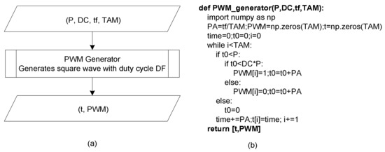
Figure 6.
Function that generates the output PWM signal: (a) Algorithm and (b) Python code.
Figure 7 shows the main function flowchart.
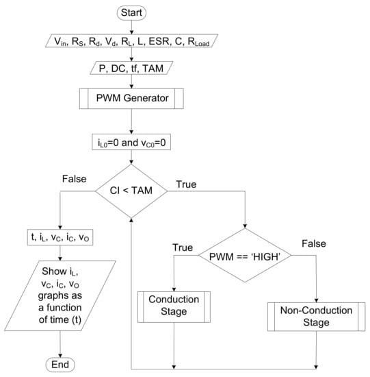
CI represents the current iteration and t, iL, vC, iC and vO represent the vectors referring to the following quantities: time, inductor current, output voltage component due exclusively to C, capacitor current and output voltage, respectively.
3. Power-Stage Design Process
To obtain design formulas for the buck converter power section, it is necessary to consider the following rules:
- Converter is operating in steady-state regime (Vin > VO);
- Average voltage across inductor is zero (⟨vL⟩ = 0);
- Average current through capacitor is zero (⟨iC⟩ = 0);
- All components are considered ideal;
- Capacitor capacitance is large enough.
Considering the converter conduction state (Figure 2), it is possible to write the following equations:
where Vin, VO, vLON, ΔiL, D, T, f, vM, iM, iD and vD represent the input voltage, mean value of output voltage, voltage across the inductor during the conduction state, inductor current ripple, duty cycle, switching period, switching frequency, MOSFET voltage, MOSFET current, diode current and diode voltage, respectively.
Considering the non-conduction state (Figure 3), it is possible to write the following equations:
From the previous equations, it is possible to compute the Di and M ratings:
- Maximum voltage value across both Di and M is equal to Vin (minimum voltage rating).
- Peak current through Di and M is equal to maximum inductor peak current (minimum current rating).
The inductor peak current can be calculated as follows:
Assuming that the average voltage across the inductor is zero, it is possible to write:
Assuming that the average value of the capacitor current is zero and neglecting the ESR effect (ESR << RLoad), it is possible to conclude that the AC component of the inductor current is equal to the capacitor current. In this way, it is possible to write:
Using Equation (5), it is possible to rewrite Equation (8) as follows
Equation (9) is commonly used to choose the capacitor capacitance. Following this, formulas that allow for the computation of the inductor inductance will be presented.
The critical inductance value takes into account the bound condition between the CCM and the DCM. The above condition occurs when the average inductor current is equal to half the ripple of the inductor current. Thus, using Equation (4), it is possible to calculate the critical value of L (Lcritical) as:
In DCM, the relationship obtained in Equation (7) no longer holds, which makes the control system more complex.
If the converter operates in CCM, as the circuit under analysis, it is usual to specify a limit to the ripple value of iL (ΔiLMax). In this case, Equation (5) can be used.
Following this, the passive components of the converter power section will be chosen considering Equations (5), (7) and (9). For this purpose, the following specifications (Table 1) will be used.

Table 1.
Power section specifications.
At first, it is important to calculate the duty cycle; so using Equation (7), it is possible to compute D:
The inductor ripple will be greater when the load current is minimum. Thus, the minimum L value can be computed as follows, using Equation (5):
Finally, it is possible to calculate C through Equation (9):
Considering the above conditions, the component tolerance and a safety margin, it was decided to choose the following passive elements:
Since the capacitance value is relatively high, an Alcap capacitor was chosen. As the ESR value of a 220 μF Alcap is in the order of 0.2 Ω at 1 kHz [26], it is possible to conclude that the output voltage ripple will be essentially the result of the ESR:
4. Simulation of the Closed-Loop Operation
In this section, the implementation of the proposed technique for a converter operating in closed loop will be shown.
At first, it is important to analyze the control circuit (Figure 8).
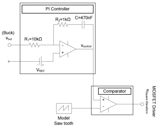
Figure 8.
Schematics of the control circuit.
As can be seen in Figure 8, the control circuit is composed of three fundamental elements: the PI controller, the Comparator and the Saw Tooth Generator.
To implement the PI controller in Python it is necessary to discretize its transfer function Equation (12):
The saw tooth generator must be implemented in a specific function (Figure 9). The function should receive as input arguments the amplitude of the Saw Tooth waveform (Amp), the period (P), the final simulation time (tf) and the total number of iterations, TAM. In turn, the function returns the time vector, as well as a saw tooth waveform with period P.
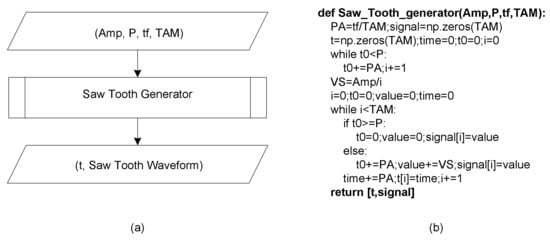
Figure 9.
Function that generates the Saw Tooth Waveform: (a) Algorithm and (b) Python code.
The comparator can be implemented through a simple control-of-flow statement (if…elif…else). The previous instruction must take into account the possibility of op-amp saturation.
Finally, the previous functions must be properly included into the algorithm presented in Figure 7.
5. Comparison—Proposed Technique versus LTspice
To show the applicability of the proposed simulation technique, a comparison of the proposed technique with LTspice will be presented in this section.
Figure 10 shows the implementation of the circuit under analysis in LTspice.
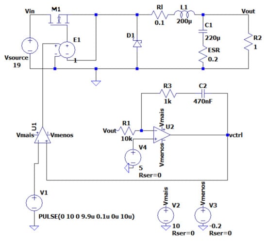
Figure 10.
Circuit implementation in LTspice.
To assess the feasibility of the proposed simulation technique, four different operating conditions are considered: steady state (Figure 11), start up (Figure 12), load variation (Figure 13) and input voltage variation (Figure 14).
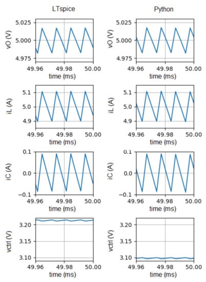
Figure 11.
Waveforms of vO, iL, iC and vctrl obtained in steady-state regime, with LTspice (left plots) and with the proposed simulation technique (right plots).
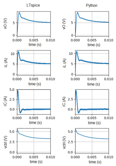
Figure 12.
Waveforms of vO, iL, iC and vctrl obtained during the converter start up, with LTspice (left plots) and with the proposed simulation technique (right plots).
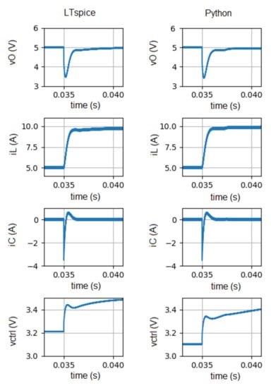
Figure 13.
Waveforms of vO, iL, iC and vctrl obtained during a load variation (from 5 A to 10 A) at 35 ms, with LTspice (left plots) and with the proposed simulation technique (right plots).
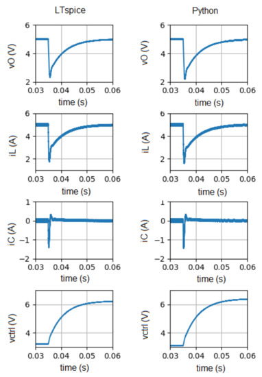
Figure 14.
Waveforms of vO, iL, iC and vctrl obtained during an input voltage variation (from 19 V to 9 V) at 35 ms, with LTspice (left plots) and with the proposed simulation technique (right plots).
Figure 11, Figure 12, Figure 13 and Figure 14 show the time evolution of vO, iL, iC, and vctrl obtained in LTspice (left plots) and also with the proposed simulation technique (right plots).
Figure 11 shows the waveforms related to the steady state regime.
Next, the results related to converter start up (Figure 12) will be presented.
Figure 13 shows the behavior of the converter when subjected to a load variation (from 5 A to 10 A at 35 ms).
Figure 14 shows the behavior of the converter when subjected to an input voltage variation (from 19 V to 9 V at 35 ms).
Figure 11, Figure 12, Figure 13 and Figure 14 show the waveforms of the output voltage (vO), inductor current (iL), capacitor current (iC) and control voltage (vctrl) obtained with the proposed technique and in LTspice. vctrl shows a slight difference between both simulations, which is essentially due to the time taken by the MOSFET to switch. This time period is not taken into account in Python simulation.
In summary, it is possible to conclude that the results of both simulators are quite similar. Thus, it can be concluded that the proposed solution can be used profitably to predict the behavior of DC-DC converters.
6. Conclusions
In this paper, a Python-based simulation technique for SMNI DC-DC converters, operating in closed loop, was presented. It was demonstrated that the proposed simulation technique can be used to predict the behavior of DC-DC converters, and for that purpose, LTspice was used to validate the results. This conclusion can be corroborated when a finer comparison is made between the waveforms obtained in LTspice and the proposed technique. Thus, regarding the average value, the maximum error is 0.01%, and as far as ripple is concerned, the maximum error is 1.8%. The errors are essentially due to the sampling period, which in the case of LTspice, is variable (variable-step). In the previous analysis, the control signal was not considered because in the simulation performed in Python, the time taken by the MOSFET to switch was not considered.
MATLAB/Simulink is one of the most commonly used pieces of software in the simulation of power converters, However, since it is a commercial software, the algorithms implemented in MATLAB are proprietary. This characteristic makes the implementation of control methods and the development of fault diagnosis techniques difficult.
The major advantage of the proposed solution is that it can be implemented in any open-source numerical computational software, making it versatile and portable. Therefore, in the authors’ opinion, the proposed simulation technique makes the implementation of control methods, as well as the development of fault diagnosis techniques in DC-DC converters, much simpler.
On the other hand, an algorithm was presented that can be used in the selection of the components that compose the power section of the converter.
Author Contributions
Conceptualization, A.M.R.A.; methodology, A.M.R.A.; software, A.M.R.A.; validation, A.M.R.A.; formal analysis, A.M.R.A. and A.J.M.C.; investigation, A.M.R.A. and A.J.M.C.; resources, A.M.R.A.; data curation, A.M.R.A.; writing—original draft preparation, A.M.R.A.; writing—review and editing, A.M.R.A. and A.J.M.C.; visualization, A.M.R.A. and A.J.M.C.; supervision, A.M.R.A. and A.J.M.C.; project administration, A.M.R.A. and A.J.M.C.; funding acquisition, A.M.R.A. and A.J.M.C. All authors have read and agreed to the published version of the manuscript.
Funding
This work was supported by the European Regional Development Fund (ERDF) through the operational program for competitiveness and internationalization (COMPETE 2020), under project POCI-01-0145-FEDER-029494 and by national funds through the FCT—Portuguese Foundation for Science and Technology, under projects PTDC/EEI-EEE/29494/2017, UIDB/04131/2020 and UIDP/04131/2020.
Institutional Review Board Statement
Not applicable.
Informed Consent Statement
Not applicable.
Data Availability Statement
The data presented in this study are available on request from the corresponding author.
Conflicts of Interest
The authors declare no conflict of interest.
References
- Jung, G.; Hosani, K.; Song, B.; Seo, D.; Kim, J.; Cho, D. Semi-Dynamic Wireless Power Charging System for Autonomous Electric Vehicle. In Proceedings of the 2021 IEEE Wireless Power Transfer Conference, San Diego, CA, USA, 1–4 June 2021. [Google Scholar]
- Mohammad, K.; Rashid, M.F.; Rahat, H.; Khan, F.; Rahman, K. Detailed Analysis of DC-DC Converters Fed with Solar-PV System with MPPT. In Proceedings of the 2022 International Conference for Advancement in Technology, Goa, India, 21–22 January 2022. [Google Scholar]
- Dias, N.; Naik, A.J. Design, Modeling and Simulation of Bidirectional Buck and Boost Converter for Electric Vehicles. In Proceedings of the 2022 International Conference for Advancement in Technology, Goa, India, 21–22 January 2022. [Google Scholar]
- Jeelani, N.; Bhat, A.H.; Mir, T.N. Comparative Analysis of Voltage Control Techniques for Single Phase AC-AC Buck Converter. In Proceedings of the 2022 IEEE International Conference on Power Electronics, Smart Grid, and Renewable Energy, Trivandrum, India, 2–5 January 2022. [Google Scholar]
- Chapparya, V.; Singh, S.P.; Dey, A. Novel Non-isolated Boost-Zeta Interleaved DC-DC Converter for Low Voltage Bipolar DC Micro-grid Application. In Proceedings of the 2022 IEEE International Conference on Power Electronics, Smart Grid, and Renewable Energy, Trivandrum, India, 2–5 January 2022. [Google Scholar]
- Stala, R.; Waradzyn, Z.; Folmer, S. Input Current Ripple Reduction in a Step-Up DC–DC Switched-Capacitor Switched-Inductor Converter. IEEE Access 2022, 10, 19890–19904. [Google Scholar] [CrossRef]
- Andries, V.; Goras, L.; Buzo, A.; Pelz, G. Automatic tuning for a DC-DC Buck Converter with adaptive controller. In Proceedings of the 2017 International Symposium on Signals, Circuits and Systems, Iasi, Romania, 13–14 July 2017. [Google Scholar]
- Prag, K.; Woolway, M.; Celik, T. Data-Driven Model Predictive Control of DC-to-DC Buck-Boost Converter. IEEE Access 2021, 9, 101902–101915. [Google Scholar] [CrossRef]
- Andino, J.; Ayala, P.; Llanos-Proaño, J.; Naunay, D.; Martinez, W.; Arcos-Aviles, D. Constrained Modulated Model Predictive Control for a Three-Phase Three-Level Voltage Source Inverter. IEEE Access 2022, 10, 10673–10687. [Google Scholar] [CrossRef]
- Nupur, N.; Nath, S. Effect of Coupling on Discontinuous Conduction Mode of Coupled Inductor SIDO Boost Converter. IEEE Trans. Power Electron. 2022, 37, 4991–5002. [Google Scholar] [CrossRef]
- Navamani, J.D.; Geetha, A.; Almakhles, D.; Lavanya, A.; Ali, J.S. Modified LUO High Gain DC-DC Converter With Minimal Capacitor Stress for Electric Vehicle Application. IEEE Access 2021, 9, 122335–122350. [Google Scholar] [CrossRef]
- Castiglia, V.; Campagna, N.; Tommaso, A.; Miceli, R.; Nevoloso, C.; Pellitteri, F.; Puccio, C.; Viola, F. Modeling, Simulation, and Characterization of a Supercapacitor in Automotive Applications. IEEE Trans. Ind. Appl. 2022, 58, 2421–2429. [Google Scholar] [CrossRef]
- Khader, S.; Hadad, A.; Abu-aisheh, A.A. The application of PSIM & Matlab/Simulink in power electronics courses. In Proceedings of the 2011 IEEE Global Engineering Education Conference, Amman, Jordan, 4–6 April 2011. [Google Scholar]
- Showers, O.; Raji, A. Modelling and Simulation of Fuel Cell Hybrid Electric Vehicle Powertrain. In Proceedings of the 30th Southern African Universities Power Engineering Conference, Durban, South Africa, 25–27 January 2022. [Google Scholar]
- Ranjani, J.; Sheela, A.; Meena, K.P. Combination of NumPy, SciPy and Matplotlib/Pylab-a good alternative methodology to MATLAB-A Comparative analysis. In Proceedings of the 1st International Conference on Innovations in Information and Communication Technology, Chennai, India, 25–26 April 2019. [Google Scholar]
- Janarthanam, K.; Kamalesk, P.; Basil, V.; Judeson, J. Electrical Faults-Detection and Classification using Machine Learning. In Proceedings of the International Conference on Electronics and Renewable Systems, Tuticorin, India, 16–18 March 2022. [Google Scholar]
- Khond, S.; Kale, V.; Ballal, M. A combined Data Mining and Machine Learning approach for High Impedance Fault Detection in Microgrids. In Proceedings of the IEEE International Conference on Power Electronics, Smart Grid, and Renewable Energy, Trivandrum, India, 2–5 January 2022. [Google Scholar]
- Sun, Q.; Wang, Y.; Jiang, Y. A Novel Fault Diagnostic Approach for DC-DC Converters Based on CSA-DBN. IEEE Access 2018, 6, 6273–6285. [Google Scholar] [CrossRef]
- Amaral, A.; Sahraqui, M. Capacitors. In Diagnosis and Fault Tolerance of Electrical Machines Power Electronics and Drives; Chapter 5; Cardoso, A.J.M., Ed.; IET-The Institution of Engineering and Technology: London, UK, 2018; pp. 195–286. [Google Scholar]
- Xia, Y.; Xu, Y. A Transferrable Data-Driven Method for IGBT Open-Circuit Fault Diagnosis in Three-Phase Inverters. IEEE Trans. Power Electron. 2021, 36, 13478–13488. [Google Scholar] [CrossRef]
- Li, Z.; Gao, Y.; Zhang, X.; Wang, B.; Ma, H. A Model-Data-Hybrid-Driven Diagnosis Method for Open-Switch Faults in Power Converters. IEEE Trans. Power Electron. 2021, 36, 4965–4970. [Google Scholar] [CrossRef]
- Zhao, M.; Li, M.; Song, S.; Hu, Y.; Yao, Y.; Bai, X.; Hu, R.; Wu, X.; Tan, Z. An Ultra-Low Quiescent Current Tri-Mode DC-DC Buck Converter With 92.1% Peak Efficiency for IoT Application. IEEE Trans. Circuits Syst. 2022, 69, 428–439. [Google Scholar] [CrossRef]
- Malik, M.S.; Khan, H.A.; Zaffar, N.A. Evaluation of a Single Inductor based Single-Input Dual-Output Buck Converter for DC Microgrid Applications. In Proceedings of the IEEE 7th World Conference on Photovoltaic Energy Conversion, Waikoloa, HI, USA, 10–15 June 2018. [Google Scholar]
- Garg, A.; Das, M. High Efficiency Three Phase Interleaved Buck Converter for Fast Charging of EV. In Proceedings of the 1st International Conference on Power Electronics and Energy, Bhubaneswar, India, 2–3 January 2021. [Google Scholar]
- Venkatramanan, D.; John, V. Dynamic Modeling and Analysis of Buck Converter Based Solar PV Charge Controller for Improved MPPT Performance. IEEE Trans. Ind. Appl. 2019, 55, 6234–6246. [Google Scholar] [CrossRef]
- Amaral, A.M.R.; Cardoso, A.J.M. A Simple Offline Technique for Evaluating the Condition of Aluminum–Electrolytic–Capacitors. IEEE Trans. Ind. Electron. 2009, 56, 3230–3237. [Google Scholar] [CrossRef]
Publisher’s Note: MDPI stays neutral with regard to jurisdictional claims in published maps and institutional affiliations. |
© 2022 by the authors. Licensee MDPI, Basel, Switzerland. This article is an open access article distributed under the terms and conditions of the Creative Commons Attribution (CC BY) license (https://creativecommons.org/licenses/by/4.0/).