Article

A Simple Method for Porous Structure Characterization of Ultrafiltration Membranes from Permeability Data and Hydrodynamic Models: A Semi-Empirical Approach


by
Manuel Palencia
1,*,
Jina M. Martínez-Lara
1,2,
Jorge M. Durango
2,
José Sebastián López Vélez
3 and
Enrique M. Combatt
4
1
Research Group in Science with Technological Applications (GI-CAT), Department of Chemistry, Faculty of Natural and Exact Sciences, Universidad del Valle, Cali 760032, Colombia
2
Mindtech Research Group (Mindtech-RG), Mindtech S.A.S, Cali 760032, Colombia
3
Fundación Instituto de Pensamiento Complejo (IPC), Manizales 170001, Colombia
4
Department of Agricultural Engineering and Rural Development, Faculty of Agricultural Sciences, Universidad de Córdoba, Montería 230002, Colombia
*
Author to whom correspondence should be addressed.
Surfaces 2026, 9(1), 5; https://doi.org/10.3390/surfaces9010005
Submission received: 2 November 2025 / Revised: 9 December 2025 / Accepted: 22 December 2025 / Published: 27 December 2025

Abstract

New approaches to the characterization of porous materials must satisfy principles of green analytical chemistry; in addition, they should be reproducible, versatile, and capable of providing relevant information for specific applications. Membrane characterization techniques often fail to meet some of these requirements. Specifically, hydrodynamic porous-based model methods (HPMMs) enable the simulation and evaluation of membrane properties, as well as the monitoring of changes in the response to controlled and uncontrolled modifications. Nevertheless, HPMMs are limited by the multifactorial relationships between their variables and by the generation of only single-value responses. Here, a semi-empirical approach to the characterization of membrane pore structure is proposed and evaluated using simple experimental measurements from pristine and modified membranes. The model enables the determination of the effective pore radius based on two size descriptors related to porosity and permeability, the construction of pore size distributions, and the estimation of structural parameters, such as the number of pores, pore size, and surface porosity. Furthermore, it allows for the simulation of Darcy-type flow behavior in both linear and nonlinear regimes. The model was evaluated on pristine and poly(vinyl alcohol)-modified poly(ethersulfone) ultrafiltration membranes (60–120 mmolL−1) by diafiltration (100–400 kPa). Results demonstrate the usefulness of the model in characterizing membrane pore structure by using simple, fast, and non-destructive methods, thereby enabling advances in analytical diafiltration for membrane characterization.

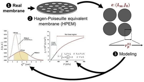
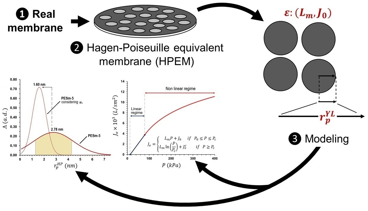
Graphical Abstract

1. Introduction

Ultrafiltration membranes (UFMs) represent a versatile technology with numerous applications. They are used in water treatment as pretreatment for other filtration operations (e.g., nanofiltration and reverse osmosis), for the removal and concentration of ions and other solutes in bioprocessing; the purification of drugs, polymers, and other substances; and operations in the food and beverage industry [1,2]. UFMs are manufactured from a variety of materials, including polysulfones, polyimines, cellulose acetate, and polyvinylidene fluoride, among others. Among commercial UFMs, poly(ether sulfone) membranes (PESms) are widely used due to their chemical resistance, mechanical stability, and ease of modification [3]. To design, optimize, and predict their performance over time, it is necessary to understand their porous structure, including their pore size distribution, effective pore size, surface porosity, pore number density, tortuosity, and active layer thickness [4,5,6]. These structural parameters govern critical functional properties, such as hydraulic permeability ( L m ), solute rejection, fouling resistance, flux decline by effect of pressure ( P ), and mechanical durability; moreover, they provide valuable insights for the scaling of membrane processes to evaluate the impact of membrane modifications and for the development of new membranes [7,8,9,10,11].
The effective pore size, defined in terms of the effective mean pore diameter or effective mean pore radius ( r p ) is the property most directly linked to the separation capacity of membranes. It is a key parameter for estimating which molecules or particles can be retained or pass through the membrane. In ultrafiltration (UF), membranes are typically characterized by the molecular exclusion cut-off, and in some cases, this parameter is related to the average pore radius, although their permeation properties are more accurately defined by pore size distribution [12]. In general terms, an excessively large pore size reduces solute rejection, while an excessively small pore size restricts flow and can increase fouling. Furthermore, pore size influences the critical blocking pressure and behavior under nonlinear regimes, for example, when cake compression or pore closure occurs at high pressures [13,14,15]. In the design of composite membranes and hierarchical structures, fine control of pore size at the active layer level is crucial to achieving high permeability and adequate rejection [16,17]. In turn, transport models require the assumption of a mean pore size to estimate aspects such as internal diffusion and convection rates in porous channels [18,19,20].
Surface porosity ( ε ) is another structural property of UFMs and is defined as the fraction of porous area relative to the total membrane surface area.
ε = A p n e t A m = V p n e t V m
where A m is the membrane area, A p n e t is the total surface area of the pores, V m is the membrane volume, and V p n e t is the total volume of the pores. Assuming cylindrical pores,
ε = n p π r p 2 A m
where n p is the number of pores, r p is the pore radius, and π = 3.1416 . But also,
ε = n p r p r m 2
where r m is the radius of the membrane, which is assumed to have a disk shape [12]. Note that (3) can be used to correct the order of magnitude of the results, since they should be consistent with ε (scaling correction): ε ~ 1 × 10 1 , r m ~ 1 × 10 2 , and r p ~ 1 × 10 9 [21]; therefore, it is expected that n p ~ 1 × 10 13 .
Surface porosity defines the density of hydraulic channels available for the passage of fluids, commonly water and dissolved solutes; moreover, according to (1), it can be interpreted as the void space contained within the membrane. For equal pore size, greater surface porosity allows for greater hydraulic flow. Furthermore, when porosity is high, the internal volume available to distribute the flow increases, and the entry velocity in each individual pore is greater, thereby mitigating the polarization effects of fluid local concentration or particle cake formation [22,23]. The number of pores per unit area ( δ p ) (or pore density) is a complementary measure used to compare membrane efficiency. Thus, two membranes can exhibit the same ε but different n p values, depending on whether the pores are larger but fewer or smaller but more numerous. The balance between δ p and size is important to optimize flow within each channel and to minimize hydrodynamic losses induced by the local interconnection of adjacent pores. A greater number of well-distributed pores improves the utilization of the membrane’s effective area and reduces entry velocity in pores [18,24]. In addition, ε and δ p influence the crossflow distribution within the support substrate in composite membranes and the uniformity of the local velocity profile, which is critical to avoiding dead zones (i.e., a membrane’s porous areas through which fluid does not pass; these areas act as non-permeable regions) or low-drag regions in porous-supported membranes [24,25].
The active layer thickness ( y m ) is the parameter influencing transport through the membrane, as it corresponds to the porous functional layer responsible for separation and flow, that is, the portion of the membrane that exerts actual hydraulic resistance. A lower thickness favors higher flow for the same pore size, reducing hydraulic resistance. However, too low a thickness value can compromise mechanical integrity or fouling resistance [1,2]. In addition, y influences how local pressure and flux velocity are distributed within the pore; thus, in long pores, the effects of internal pressure drop (i.e., gradients within the pore channel) can be significant, whereas in shorter pores, the pressure drop can be considered uniform [26,27,28]. In asymmetric membranes, the transition interface between the support and active layers also contributes to the total thickness and can introduce hidden resistance, thereby limiting effective permeability and affecting ion rejection [29,30,31].
On the other hand, tortuosity ( τ ) is a measure of how indirect, or nonlinear, the path of a water molecule passing through the porous medium is, compared with a straight path defined from one side of the membrane to the other. It is described as the ratio of the internal path, or effective pore path ( y p ), to the membrane thickness.
τ = y p y m
High tortuosity implies that pores bend, bifurcate, or branch extensively, thereby increasing hydraulic resistance for the same pore size. Even with relatively large pores and good porosity, high tortuosity can significantly restrict flow [32]. Tortuosity also influences solute diffusion within the pore, concentration polarization and the resistance resulting from local diffusion. In membrane transport models, the inclusion of a tortuosity factor is essential to correcting effective diffusion within the pore relative to that in the free solution; moreover, in membranes with a hierarchical structure, the tortuosity of the supporting substrate can be as critical as that of the active layer [32,33,34].
Due to the micro- and nanoporous nature of membranes, characterized by relatively high spatial microheterogeneity, variable pore morphology, small thickness for proper functionality, and the changes they undergo during operation, the characterization of their structural parameters is inherently complex. For example, although techniques such as scanning electron microscopy (SEM), transmission electronic microscopy (TEM) or atomic force microscopy (AFM), and mercury porosimetry are widely used, they provide only information about the membrane in a non-operational state. In addition, although the geometric pore size can be determined by SEM or AFM, this value is unrealistic under operating conditions because permeation properties will be the result of a smaller pore size. Consequently, the information provided by SEM or TEM corresponds more closely to an average maximum pore size limit than to the effective mean pore radius [35,36,37,38].
Typical problems arising during analysis of membrane structural properties are related to their heterogeneity; for example, when point measurements are performed using SEM, TEM, or AFM, there is a risk that the analyzed area does not represent the region of interest under real operating conditions [37,38]. In addition, sample preparation steps such as cutting, drying, impregnation with contrast fluids, and the use of coating scan alter or collapse the original structure of the membrane. Many porous membranes undergo deformation under pressure-based measurement techniques (e.g., porosimetry and capillary pressure), which biases the results toward smaller apparent pore sizes. Some techniques, such as porosimetry, do not distinguish between pores that that contribute to actual flow and inaccessible internal cavities, dead zones, or non-functional regions [24]. When tracers or gases are used, diffusion or permeation may be affected by adsorption, internal diffusion retardation, or wall effects, which are directly related to the nature and chemical composition of membranes. In imaging-based techniques, many pores or their internal connections in the nanometer range are not adequately captured, leading to underestimated results [39,40]. Another aspect that often goes unnoticed is the difference between the standard conditions under which measurements should be performed and the conditions under which the membranes are used. This leads to a lack of information on the effect of in situ variables such as pH, temperature, humidity, ionic strength, and others [13,41]. This means that many results are nominal or referential and therefore do not provide a faithful description of the membranes under the conditions of interest. Different methods for determining various structural parameters of membranes are reported in Table 1.
Note that membrane characterization using conventional methods such as mercury porosimetry, liquid–liquid displacement porosimetry, and SEM can deviate from several principles of green analytical chemistry. The main advantages of the proposed method are the use of water as the working fluid and the possibility of reusing the membrane (i.e., it is a non-sample-destructive method). This contrasts with techniques such as mercury porosimetry, which uses mercury, a well-known highly toxic element. Other techniques, such as liquid–liquid displacement porosimetry, use solvent mixtures like isobutanol, methanol, isopropanol, chloropentane, pentanol, and octanol to wet the surface, which can cause membrane swelling, distort the results, and even destroy the sample. These solvents have a higher relative toxicity than water, and their difficult recovery increases the environmental footprint of the analysis. In addition, techniques such as SEM have high energy consumption, specifically to maintain vacuum conditions. They also require the vaporization of metals for coating operations, which must be vaporized; these include Au, Pd, and Pt. In both porosimetry and microscopic-based techniques, samples cannot be reused, which increases waste generation. Furthermore, other aspects, such as the environmental costs of manufacturing and maintaining these techniques, should be highlighted.
On the other hand, equations describing permeability ( L m ), ε , and flow behavior, although well established, involve significant oversimplification, usually related to geometric assumptions [42,43,44]. Recently, new approaches based on more complex mathematical methods in conjunction with computational tools have been proposed, and although these are interesting, like high-resolution microscopic techniques such as SEM, TEM, and AFM, although they are useful for investigations, they are often impractical for industrial processes due to their high cost, which is frequently a limiting factor [45,46,47,48]. Therefore, semi-empirical approaches offer a lower-cost alternative that can minimize the effects of oversimplification while providing a more realistic description of the processes, since data are acquired under real operating conditions. Currently, many semi-empirical models have been developed; a recent review describes around 63 different models, developed for a wide range of specific conditions and phenomena [49]. Their complexity varies, and their usefulness depends on the researcher’s interest. They all start from the same basic set of laws or mathematical relationships, generally Darcy’s law, the Hagen–Poiseuille equation, and the inverse relationship between hydraulic permeability and resistance, among others. However, these models mainly focus on describing and predicting membrane flux, fouling, permeability, and resistance. They are, therefore, not usually applied to the structural characterization of membranes, but rather to the analysis of transport, retention, and fouling processes (mass transport coefficient, pore blockage, filter cake formation, flux prediction, and concentration polarization). The restriction on the use of these models for structural membrane characterization is due to the multifactorial relationships among membrane structural variables. In particular, the relationship among L m , ε , r p , and n p is particularly complex due to their strong interdependence.
In this study, a semi-empirical approach to structural membrane characterization based on simple experimental measurements is proposed and evaluated using both pristine and modified membranes.

2. Details on the Modeling of Porous Membrane Structure

As a starting point, the concept of the Hagen–Poiseuille equivalent membrane (HPEM) is introduced. This membrane is flat, with evenly distributed cylindrical pores and a permeability equal to that of the real membrane. Under this premise, every membrane has an equivalent membrane that, although it may differ in shape, has structural characteristics that result in the same permeability. This concept also allows for the definition of a reference point from which comparisons can be made. Although this is not developed further in this document, a reference HPEM could, for example, be defined as one having L m = 8 μ y = 1   s m 1 (or L m 1 s P a 1 ) at 25 °C.
According to the Young–Laplace equation, the pressure ( P ) necessary to force the passage of fluid through a membrane depends on r p , the surface tension ( γ ), and the contact angle ( θ ) at the liquid–solid interface [24]; for water, this is given by
P = 2 γ w c o s ( θ w ) r p
where γ w and θ w are the surface tension and contact angle of water, respectively. Furthermore, since membrane pore sizes are very small, P must exceed a minimum pressure ( P 0 ), which depends on the membrane permeability characteristics; here, P 0 is defined to be related to a dry membrane prior to hydration. By replacing r p from (5) into (2), it follows that
ε = π n p A m 2 γ w c o s ( θ w ) P 0 2
In addition, the Young–Laplace radius ( r p Y L ) is defined to be the radius related to L m through P 0 . Thus,
r p Y L = 2 γ w c o s ( θ w ) P 0
This definition is useful because it simplifies the equations, as it is a recurring term in many of them; in addition, it is necessary later for model prediction and interpretation. Thus,
ε = π n p A m r p Y L 2
On the other hand, for the HPEM, L m is given by
L m = ε r p 2 8 μ y
By combining (7) and (9), we obtain
L m = ε 8 μ y 2 γ w c o s ( θ w ) P 0 2
L m = ε 8 μ y r p Y L 2
where μ is the viscosity of the fluid. Thus, by experimental determination of P 0 , L m , and θ w , ε can be easily estimated.
According to Darcy’s law, which is commonly represented by a flux-versus-pressure plot ( P ) , or J v : ( P ) plot, the volumetric flux ( J v ) is directly proportional to P at low pressures, that is, J v = L m P (linear regimen); however, as P increases beyond the critical value of P ( P c ), linearity is lost (nonlinear regimen), and the flux decreases until it reaches a plateau. Therefore, from Darcy’s formulation, L m = d J v / d P .
Hence, if (10) is generalized for any value of P , it is concluded that
L m P = J v = ε k θ Y L 2 8 μ y 1 P
Obviously, the equality does not hold for the same values of P , except at P = 1 , because the left side of (12) defines a linear flow behavior (linear regime of the J v : P plot) and therefore the values of P P c , whereas the right side defines a nonlinear behavior (nonlinear regime of the J v : P plot), corresponding to P P c . However, Equation (12) is shown to explicitly illustrate the deductive reasoning underlying the previous conclusion. Here, k θ Y L = 2 γ w c o s ( θ w ) . By re-writing (12), we have
J v = L m P i f   P 0 P P c ε k θ Y L 2 8 μ y 1 P i f   P P c
From (13), L m in each regime can be defined: L m = d J v / d P (linear regime) and L m = d J v / d 1 / P (nonlinear regime). By integrating the above, we have
J v = L m P + J 0 i f   P 0 P P c L m ln P P c + J v c i f   P P c
The integration limits used are, for the linear regimen, J 0 J v and P 0 P , and for the nonlinear regimen, J v c J v and P c P . Implicitly y was assumed to be constant. The above is a valid approximation when water is used as the working fluid, so there is no concentration polarization or fouling. In addition, it is assumed that membrane compression is absent, which is valid if pressures above P c are kept relatively low. Thus, (14) is completely consistent with experimental data, and its importance is demonstrated in the Section 4.
On the other hand, ε can be calculated from (11), whereas two expressions are possible for r p : one derived from (9) (Hagen–Poiseuille equation) and another defined by (7) (Young–Laplace equation). By introducing the Hagen–Poiseuille radius ( r p H P ), we obtain
r p H P = 8 μ y L m ε 1 / 2
Also, two expressions are possible to obtain n p . From (8),
n p = ε A m π r p Y L 2
and by combining (2) and (9),
n p = 8 μ y A m L m π r p Y L 2 r p H P 2
From (17), it can be seen that r p is the geometric mean ( r p g ) calculated from r p L Y and r p H P . Thus,
r p g 2 = r p Y L 2 r p H P 2
In other words, the conclusion that the geometric mean, rather than any other parameter, should be the descriptor of the mean value of effective pore radius arises directly from the underlying assumptions of the model, rather than from physical or statistical interpretations. By defining two radii instead of one and showing that they converge to the same expression, it is interesting to note that the use of the geometric mean appears as a natural descriptor in the model. Finally, it is concluded that
n p = 8 μ y A m L m π r p g 4
However, the results indicate that a better description of n p is obtained using r p H P derived from (17).
Note that it is implicitly assumed that the flow, although not strictly laminar, occurs in pores that are sufficiently small for inertial effects to be negligible. However, this assumption can be verified by determining the Reynolds number. In UF membranes, pore size is at the nanometer scale; therefore, even at high flow rates, the Reynolds number is less than 1 (in our case, Re ~ 2.3 × 10⁻⁷).
The approach proposed here is based on deriving the result through sequential approximations, which are based on scale criteria and congruency between equations. Further details are provided in the Section 3.

3. Materials and Methods

3.1. Reagents and Equipment

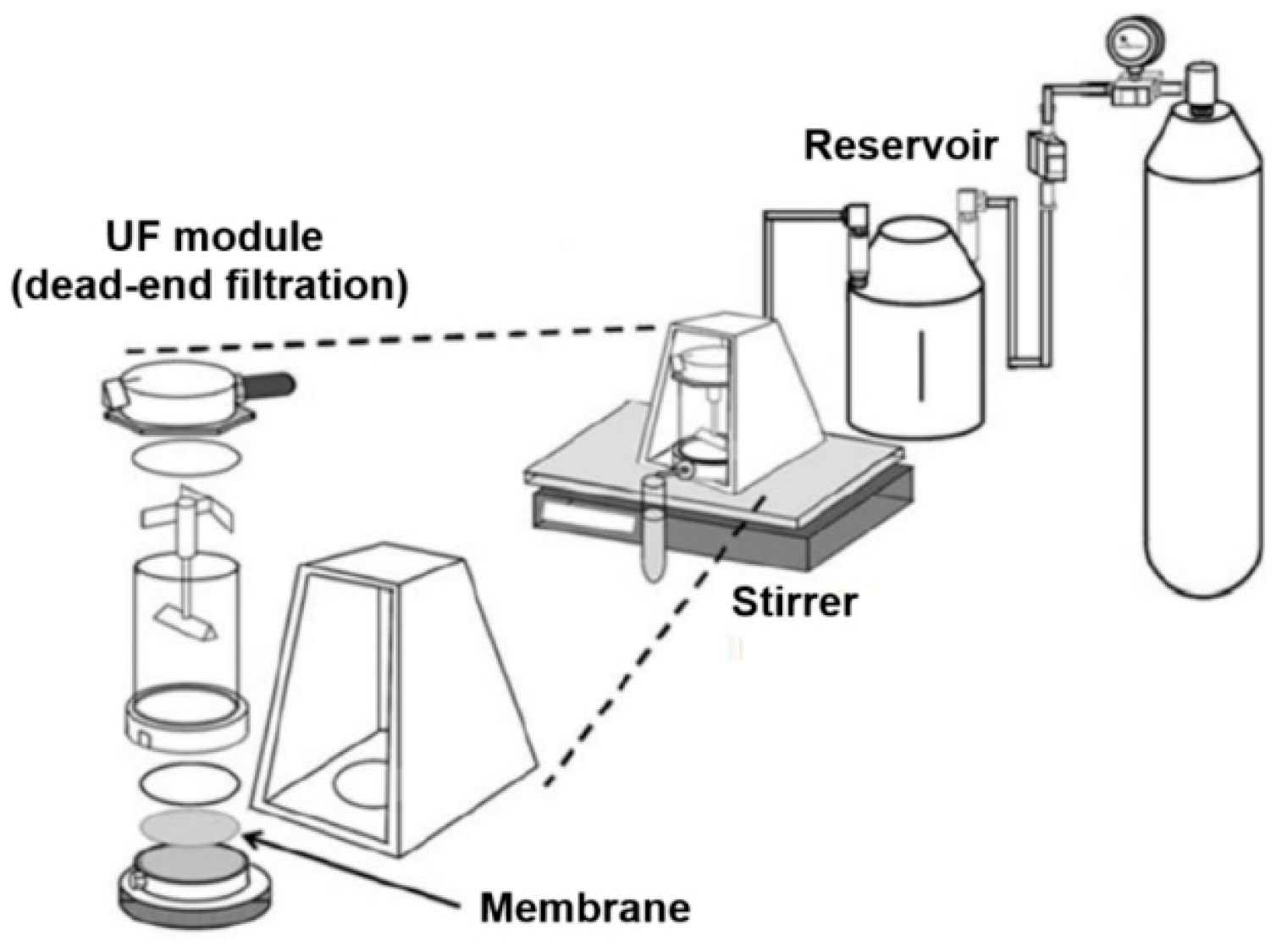
Ultrafiltration membranes of poly(ether sulfone) (PESms) were used for filtration experiments (Millipore, NH, USA; molecular weight cut-off of 10 kDa). These membranes are asymmetric membranes made from a thin layer of PES on a microporous layer of polypropylene. Deionized water (Milli-Q, Germany) was used in hydraulic permeability tests. Pristine membranes were used in all experiments. Poly(vinyl alcohol) (PVA; 30   k D a ; Aldrich, MO, USA) was used as a surface modification agent. Permeability tests were performed using a dead-end UF system including one stirred-cell UF module (Amicon, MA, USA; maximum volume of 50–60 mL), one feed tank with the capacity of 1 L, one pressure source (N2 was used), one pressure gauge, and one control valve for the flow of water or gas from the reservoir to the filtration cell (see Figure 1).

3.2. Hydraulic Permeability Tests and Membrane Surface Modification by Diafiltration

Hydraulic permeability tests were performed according to the following sequence: (i) The membrane was hydrated for 2–3 h before use. (ii) The membrane was installed in the filtration unit, and water was passed from the reservoir to the filtration cell for removing additives. (iii) Flow’s measurements started from the highest pressure and subsequently decreased to the next pressure (working pressures were 100, 200, 300, and 400 kPa, and the stirring rate was 250 rpm); for this purpose, UF was performed using continuous diafiltration by the washing method (i.e., water is fed from the reservoir to the filtration cell while maintaining a constant volume at all times) [50]. (iv) A mass of water was collected in previously weighed tubes, and the permeate time was measured with a stopwatch. (v) Filtration was stopped, the water inside the cell was removed, and 50 mL of a PVA solution were added (60.0 mmol/L with respect to repeating units; in addition, the polymer concentration was sufficiently low to ensure a diluted regime). (vi) Filtration was restarted in washing mode; thus, precipitation, filtration cake formation, and gelation of polymer were avoided. The purpose of this step was to slightly modify the membrane surface to alter its permeation properties by decreasing r p and/or n p . (vii) After collecting ~50 mL of permeate, filtration was stopped, the polymer solution was removed from the cell, the system was rinsed with deionized water without disassembly, and steps (i)–(iv) were repeated for each pressure. (viii) The entire sequence from steps (i) to (vii) was repeated until three replicates were completed, and each replicate was performed using a pristine membrane. (ix) Finally, the entire sequence from steps (i) to (viii) was repeated using PVA solutions with concentrations of 80.0, 100.0, and 120.0 mmol/L at a pressure of 400 kPa. This pressure was selected because it lies within the working pressure range of UF equipment, which has a maximum operating pressure of 550 kPa. Furthermore, it is the maximum pressure used in the permeability tests. At higher pressures, deformation of the internal porous structure of the membrane and PVA fouling within the pores may occur. This is reflected in the reduction in surface porosity (see Section 4.2.3 and Section 4.3 and Supplementary Information in Table S1).

3.3. Data Processing

Some parameters were obtained from previous publications and used in modeling calculations as comparative information (see Table 2). In addition, J v : P plots were obtained for each membrane before and after contact with PVA solutions. A linear correlation was used for pristine membranes, whereas a logarithm correlation was applied to the modified membranes, as described in (14). Thus, the membrane structure was established before modification.

Determination of Membrane Structural Characteristics

The calculation sequence for pristine membranes can be performed in two ways: one, here named “forward scaling”, is based on the use of P 0 to find r p Y L (i.e., P 0 r p Y L , followed by the re-scaling method applied to ε , n p , and r p H G ), and another, here named “backward scaling”, is based on the use of P 0 to find r p Y L , followed by the re-scaling of r p Y L and then the correction of P 0 ( P 0 * ) (i.e., P 0 r p Y L , followed by the re-scaling method applied to ε , n p , and r p H G , and finally, r p Y L P 0 ).
(A)
Forward-scaling method steps are described below:
  • L m and J 0 are obtained from the linear correlation of the J v : P plot.
  • P 0 is obtained from P 0 = J 0 / L m .
  • r p Y L is obtained from (7).
  • The first approximation of ε is obtained with (10); however, it is necessary to introduce a scaling factor ( s ε ) due to (3). The new equation is given by
    ε = 8 v w s ε L m ( r p Y L ) 2
    where v w is the water flux rate at 25 °C and s ε = 10 1   o r   10 2 . s ε is required to satisfy that 0 < ε < 1 .
  • The first approximation of r p H P ( r p , 0 H P ) is obtained with (15).
  • The first approximation of n p ( n p 0 ) is obtained with (16) or (17).
  • According to (2) (scaling correction), a scaling factor ( s n ) may be introduced. Thus, s n can be easily determined as
    s n = 1 × 10 m
    where n p = s n n p 0 and m = 12 n or m = 13 n , with n being the exponent obtained for n p 0 ( n = ± 1 ).
  • r p H P is re-calculated by modifying (15) to be
    r p H P = 1 r p Y L 2 8 v w A m L m π s n n p 0
  • s n values satisfying expected conditions are sought. In our case, for PESms with a cut-off of 10 kDa, r p cannot be lower than 1 nm, but also it should be lower than 8–10 nm. From the data analysis, it was concluded that this condition corresponds to a change in n of ± 1 . Note that in item 7, a first value which can be an upper limit ( r p , u H P ) or lower limit ( r p , l H P ) for r p H P was found.
  • r p H P and r p Y L must satisfy (18), being an implicit characteristic in (9). Thus, geometric r p or mean surface pore radius ( r p ) is defined as the geometric mean according to (18).
(B)
Backward-scaling method steps are described below:
  • L m and J 0 are obtained from the linear correlation of the J v : P plot.
  • P 0 is obtained from P 0 = J 0 / L m .
  • r p Y L is obtained from (7) modified by s Y L , i.e., r p = s Y L r p Y L , with s Y L = 1 × 10 3 .
  • ε is obtained with (20) but using s ε = 1 × 10 5 .
  • The first approximation of r p H P ( r p , 0 H P ) is obtained with (15).
  • The first approximation of n p ( n p 0 ) is obtained with (16) or (17).
  • According to (2) (scaling correction), in (21), n p = s n n p 0 , and m = 12 n or m = 13 n , with n being the exponent obtained for n p 0 ( n = 1 ).
  • r p H P is re-calculated using (22).
  • s n values satisfying expected conditions are sought. From the data analysis, it was concluded that this condition corresponds to a change in n of ± 0.1 .
  • According to this procedure, the values of r p H P , n p , and ε are the same as those obtained by forward scaling. But, in this path, r p Y L = r p H P = r p ; however, the relationship between r p and P 0 cannot be adequately predicted. Thus, while forward scaling absorbs this difference, causing r p Y L r p H P , by backward-scaling, this difference is transferred to P 0 .

3.4. Impact of Experimental Error on Results

To evaluate the impact of experimental errors on the prediction of P 0 , a dataset obtained from one of the linear models was used as a reference. The use of one linear model ensures that all errors present in the simulated data arise from the simulation itself and are not errors inherited or transmitted from experimental measurements; in addition, it allows the simulation to work in the same scale order as the empirical data. Next, a generating function of random error ( F ϵ ) was used to introduce stochastic perturbations into the variables. Thus, the effect of random error on the results was analyzed by controlling a maximum and minimum threshold ( ϵ m a x and ϵ m i n , respectively). Here, f ϵ is given by
F ϵ ϵ n , n = ϵ n ϵ n ϵ n ϵ m a x ϵ m i n
where ϵ n is the random error resulting from the difference of two consecutive pseudo-random events ( ϵ 1 and ϵ 2 , respectively), i.e., ϵ n = ϵ 2 ϵ 1 , with ϵ 1 and ϵ 2 being random numbers ranging between 0.000 and 1.000; therefore, ϵ n 1 ,   1 . In addition, ϵ n ϵ n 1 , ϵ m a x ϵ m i n , and ϵ n determine randomly the sign (i.e., direction), scale, and direction, respectively. Thus, f ϵ generates a random perturbation on a variable with a percentage relative absolute error ranging between ϵ m a x and ϵ m i n . Finally, for one x variable, random perturbation ( y ) is given by
y = x + f ϵ 100 x
where f ϵ is the random error defined by F ϵ ϵ n , ϵ m a x .
For the simulation, random errors of the variables under analysis (i.e., P , w , and t ) were simulated using (23) and (24), and subsequently, the new values were introduced into the linear model to obtain the magnitude of the error on L m , J 0 , and P 0 . By applying (23) and (24), the Excel Microsoft function “= random ()” was used to produce the values of ϵ 1 and ϵ 2 . The thresholds evaluated were ( ϵ m a x % = 1 , 2   a n d   5 with respect to P (in kPa), w (in kg), and t (in c s ) and ϵ m i n % = 0 in all cases). Percentage relative absolute deviation ( ϵ r a d ) and mean square deviation ( ϵ m s d ) were used as error indicators; they were obtained by averaging ϵ r a e and ϵ m s d over 20 simulation cycles; in addition, the maximum possible error was set as the largest value observed within the observation window ( ϵ ¯ o b s and ϵ o b s m a x , respectively).

3.5. Pore Distribution Modeling

To simplify the notation, r p , l H P r p , 1 , r p , u H P r p , 2 , and r p ¯ = r p , 2 + r p , 1 / 2 . Two distributions were evaluated. In the first case, the normal distribution ( Λ ) is given by
Λ = 1 2 π 0.5 σ r e x p ( r p r p ¯ ) 2 2 σ r 2
where σ r is the standard deviation. For the normal distribution, two approaches were performed: (i) considering only values of r p to describe the distribution and (ii) considering r p and n p . In this case, the values of n p were used to define the weight ( w n ); thus, w n 1 = n p , 1 / n p , 1 + n p , 2 , and w n 2 = n p , 2 / n p , 1 + n p , 2 .

3.6. Darcy’s Curve Modeling for Linear and Nonlinear Regimes

In (14), the behavior of J v was shown to be described by two regimes: linear and nonlinear regimes. Thus, the nonlinear flux ( J v n l ) is described as
J v n l = ϕ m ln P + J v c ϕ m ln P c
J v n l = ϕ m ln P + J v , o b s c
with
ϕ m = ε k θ Y L 2 8 μ Δ y
J v , o b s c = J v c ϕ m ln P c
where ϕ m is the slope and is understood to be a constant, while J v , o b s c is the observed critic volumetric flux obtained for P c .
The procedure to obtain P 0 , P 0 n l , and P c is described below:
  • The J v : P plot is modeled using (14) and the cubic function given by
    J v n l = n = 0 n = 3 m n P n
    where m n denotes the coefficient with respect to the power n . Thus, from (14), we obtain P 0 n l at J v n l = 0 , whereas from (30), we obtain P 0 at J v n l = 0 using numeric methods.
  • From the above analysis, two points in the linear regimen are found and used for linear modeling.
  • The linear model is projected onto (14), since it is tangent to it. Thus, P c is obtained by replacing the respective value of J v n l ( = J v , o b s c ) in (14).

4. Results and Discussion

4.1. Analysis of Hydraulic Permeability Test of PESms

Examples of three hydraulic permeability tests on pristine membranes are shown in Figure 2. The models describing all results are summarized in Table 3 by using linear correlation parameters. In general, the behavior of the J v : P plot is as expected in all cases; that is, the membranes operate in a linear regime described by Darcy’s law. Results evidence that the selection of membranes with alike nature and the same molecular weight cut-off does not warrant the reproducibility of results in terms of P 0 because PESms are characterized by an inherent variability in terms of P 0 , and consequently, for small samples, the impact on reproducibility can be significant.
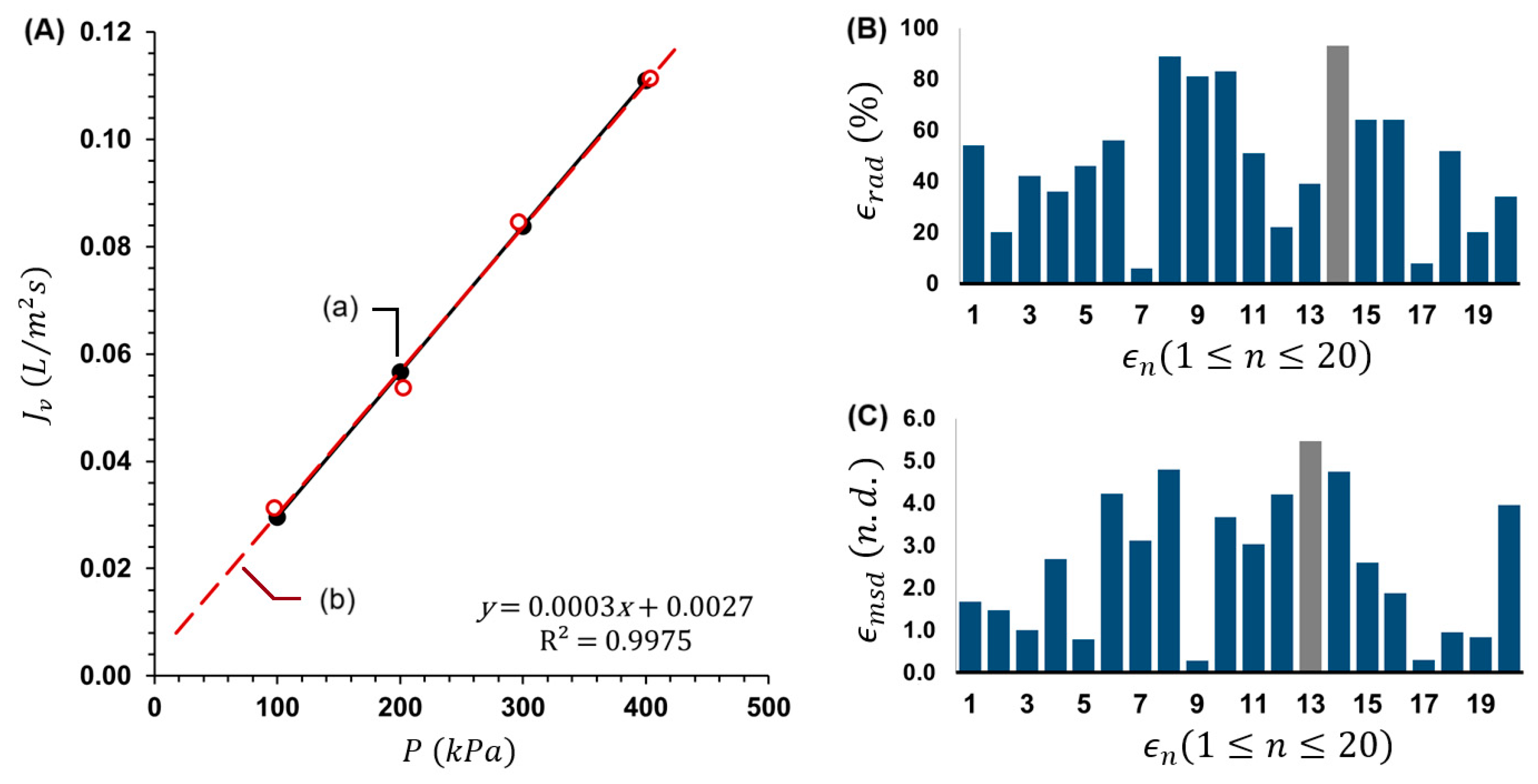
Results of random error evaluation on quality in the determination of L m and P 0 are shown in Table 4 and Table 5. In general, L m was the most stable parameter in all cases, as for this parameter, the impact of random errors on the measurements of P , t , and w is minimal within the maximum threshold evaluated. In contrast, the value of P 0 showed greater dependence on random errors that may arise during the hydraulic permeability tests (see Table 5). In addition, one example of perturbations on linear models using (23) and (24) are shown in Figure 3. According to the results, pressure is the variable of greatest concern, since the error in P 0 exceeded the defined threshold in some simulations. These results highlight the need for special care in pressure measurements, which in practice can be resolved by using manometers with the indicated accuracy. Furthermore, since the L m values are robust and the P 0 values can be obtained from carefully conducted experiments, the differences in the values shown in Table 3 cannot be entirely explained as results of internal variability within the experiments. Therefore, the variability in results is attributed to inherent variability of PESms, including variations in their porosity, pore shape and size, active layer thickness, and tortuosity.

4.2. Structural Characteristics of Pristine PESms

4.2.1. Results of Forward-Scaling Method

The values of r p Y L , r p Y L , ε , r p , 0 H P , n p 0 , n p , and r p H P describing all sequence of steps for the characterization of PESm-1, PESm-2, and PESm-3 are shown in Table 6. To simplify the analysis, results and discussion are shown for one membrane, are then compared with a small set of data, and are then generalized for all sets of PESms used.
For PESm-1, r p Y L = 3.99   μ m , which is small compared with commercial microfiltration membranes (e.g., ~12.3 μm for polypropylene membranes) and large compared with UF membranes. In addition, for ϵ r a d = 2 % , and considering ϵ o b s m a x , r p Y L ranges between 2.07 and 4.57 μm. From (7) it can be seen that r p Y L is derived directly from the fluid properties and J v : P plot, suggesting that the membrane is highly hydrophilic, and it is possible that the apparent radius may result from lower resistance to the passing of water. Typically, PESms contain various additives to improve their surface hydrophilicity, with the addition of poly(vinyl pyrrolidone) between 2 and 10% being common [52]; consequently, a decrease in θ w is related to an increase in L m , and an HPEM with a larger pore radius is modeled. Therefore, r p Y L is an apparent radius directly related to L m rather than to the real size of the pores. According to this argument, permeability characteristics are transferred to a single value, which corresponds to maximum value of r p ; that is, an HPEM with a pore size described by r p Y L will have the experimentally measured L m , from which P 0 is derived; however, there may be another HPEM with the same L m but with a smaller r p , which is possible physically by increasing n p . In this way, the analytical problem consists of reducing the pore size through progressive approximations until the minimum possible value is reached; this must be consistent with both equations and scale requirements.
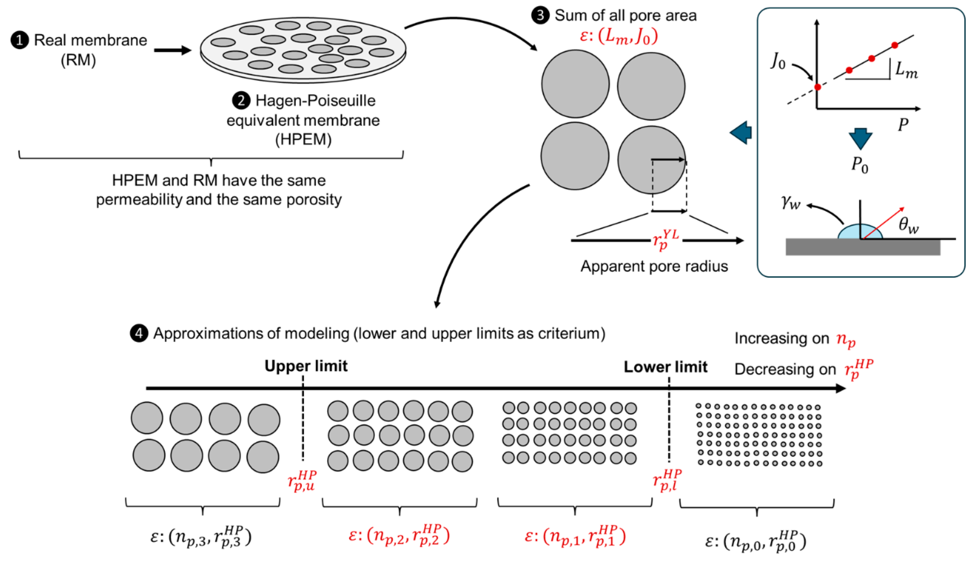
An illustration of how the model obtains the results is shown in Figure 4. For PESm-1, ε = 13%; therefore, PESm-1 can be considered a relatively dense membrane. The value of ε obtained is reasonable in terms of its magnitude, so it is important to highlight that its value is obtained from fluid properties ( μ and γ ), membrane properties ( y ), the balance of adhesive and cohesive forces between water and the membrane material ( θ w ), and the experimental information obtained from the J v : P plot ( L m and J 0 ). Furthermore, the scale factor is derived directly from (2). The values of r p Y L suggest that it the order L m : PESm-3 > PESm-1 > PESm-2 should be expected, which is consistent with the experimental values obtained. However, although the same order is concluded from ε , the relationship between the values in both cases is not linear. That is, L m k r p Y L and L m k ε , with k = constant. This line of analysis is discussed in more detail later. On the other hand, r p H P is related to ε in terms of total pore volume with respect to membrane volume.
By re-scaling, two values satisfy (20) at the same time and comply with the expected conditions defined by lower and upper limits ( r p , 1 H P and r p , 2 H P such that r p , 1 H P < r p , 2 H P ); consequently, the solution obtained for the problem of the determination of r p Y L is not a single point but a range, because of all values of r p H P within r p , 1 H P r p H P r p , 2 H P are satisfactory. Therefore, in terms of pore size distribution, it is suggested that a membrane’s heterogeneity descriptor is given by
Δ r p = r p , 2 H P r p , 1 H P
where Δ r p is the width of the pore size distribution. Thus, from (31), it is concluded that the pore size distributions for PESm-1, PESm-2, and PESm-3 show great differences in their porosities (with a variation coefficient of 39.2%) (see Table 6).
In addition, it is seen that r p H P is not a good descriptor of L m , contrary to what is observed for r p Y L ; but also, r p H P is a good descriptor of ε , contrary to what is observed for r p Y L . The mean surface pore radius for PESm-1, PESm-2, and PESm-3 is close to previously reported values [45] (see Table 2).
Two r p values to describe the membrane pore size might seem strange; however, it should be remembered that size and shape descriptors are generally concepts of equivalence, not absolute values, especially in systems characterized by a shape distribution [53,54]. Thus, r p Y L corresponds to the radius that a membrane must have to show a permeability equal to that experimentally measured for the real membrane; consequently, it is a parameter allowing one to describe the maximum surface porosity (here defined to be equal to ε 0 ). On the other hand, r p H P is the radius describing a membrane with the same permeability and porosity estimated for the real membrane but with a different pore distribution, so that the scaling conditions and defined pore size limits are satisfied. Consequently, this method requires prior information to properly calibrate the pore size thresholds.

4.2.2. Results of Backward-Scaling Method

This method is based on applying a scaling factor to r p Y L , which in principle breaks the direct association of its value with the experimental data defined by Equation (7). The introduction of s Y L triggers an increase in the value of s ε to satisfy the scaling correction deduced from (2). However, regardless of these changes, the relationship between the variables remains the same and the results are the same as those obtained using the forward-scaling method, except for r p Y L . This is explained because the values of n p and r p H P are derived from ε , which is re-scaled in both cases between 0 and 1 and remains numerically identical. Clearly, the scaling factors are the parameters that are changing. For PESm-1, PESm-2, and PESm-3, the respective calculation sequence is summarized in Table 7.
Using this method, r p Y L is equal to r p , u H P , and one characteristic is that this equality holds when s n = 10 0 . Thus, when P 0 is re-calculated for the full consistency of r p Y L using (7), it is necessary to introduce two intermediate concepts: apparent P 0 , which is obtained from the J v : P plot, and effective P 0 ( P 0 * ). These concepts are necessary to avoid the overmagnification of P 0 ; therefore, P 0 * is a scaling correction. Consequently,
P 0 = P 0 * s Y L
By comparison of the results in Table 6 and Table 7, it is concluded that two methods converge completely when s Y L is introduced into the forward-scaling method. Consequently, the overall effect is that while the forward-scaling method first finds r p , 1 H P and then r p , 2 H P , the backward-scaling method does the opposite, first estimating r p , 2 H P and then r p , 1 H P .

4.2.3. Evaluation of Generalization of Modeling: Linear Regime

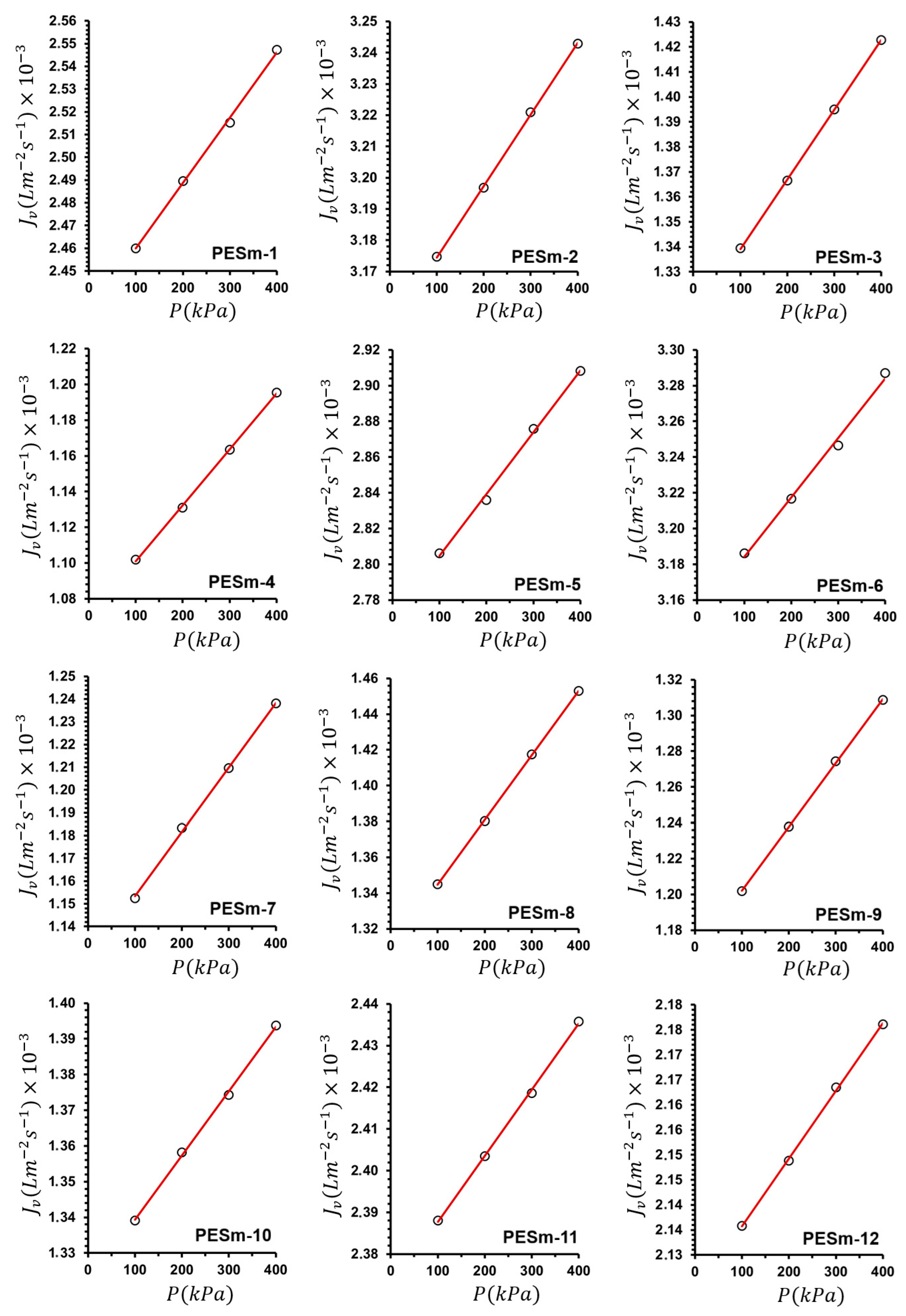
Model behavior was carried out for a set of 12 PES membranes (see Table 8). In addition, the J v : P plots for PESm-1 to PESm-12 are shown in Figure 5. The linear modeling for each membrane is shown in Table 9. Values of ε ranged from 13.0 to 55.5%, reflecting a wide variability in porosity characteristics. Similar observations in terms of variability among membranes were observed for the other parameters.
Regarding modeling, it showed the same behavior in all samples, which allowed us to define all parameters, and for pore radius, in all cases, we observed two values. Therefore, by direct comparison, it is observed that r p Y L is equal to r p , 2 H P when s Y L is used (i.e., r p , 2 H P = s Y L r p , 2 Y L ).
Thus, from the backward-scaling method, it is concluded that membranes are defined by two pore sizes acting as upper and lower limits ( r p Y L and r p H P , respectively). The above reflects several aspects of the model: (i) the differentiation of two pore radii is still necessary regardless of the scaling method used; (ii) the backward-scaling and forward-scaling methods are two different routes to achieve the same results; (iii) since r p H P corresponds to the lower limit and r p Y L corresponds to the upper limit, the description of r p as geometric mean between both radii is still necessary, which is consistent with (18); (iv) for the application of this modeling approach, prior information is required to determine the thresholds that delimit the solution set (i.e., information that can be used as calibration is required).
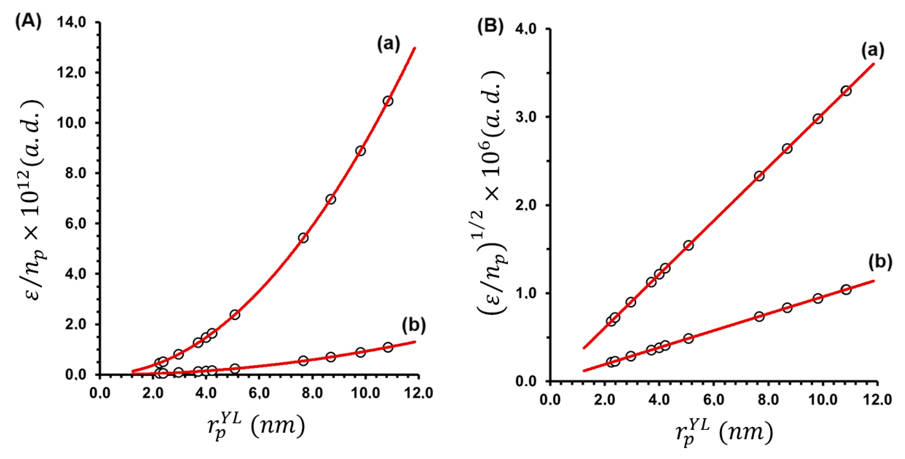
From the ordered values of r p Y L , a coherent relationship can be obtained from ε / n p as a function of r p Y L (see Figure 6A). Thus, the corresponding modeling is given by
ε n p = α r p Y L 2
where α is a constant. This behavior is predicted by (3); consequently, from (33), it is concluded that ε / n p 1 / 2 in function of r p should be described by a linear model (see Figure 6B).
In addition, the combinations of other variables do not show any trends. The above suggests that α should be analyzed in more detail, and since α 0.5 appears as a result of the overall behavior of all membranes, it is concluded that it must be associated with a common characteristic associated with all of them. By comparison with (3), it is concluded that α 1 = 10 / r m and α 2 = 10 / r m ; but also, α 2 / α 1 = 10 . The relationship with 10 is a consequence of the scale factor used. By defining an experimental ε to be ε e , it is seen that ε e = ε s ε , since s ε = 10 , and by combining this with (3), we obtain α 1 . From these relationships the prediction of r m is completely satisfactory: the calculated r m from A m is 0.0328976 m, while the r m obtained from α 1 and α 2 is 0.0328979 m (the sequence of decimals was extended in order to show the difference in the calculation; thus, the error was close to 0.001%).

4.2.4. Simulation of Pore Size Distribution

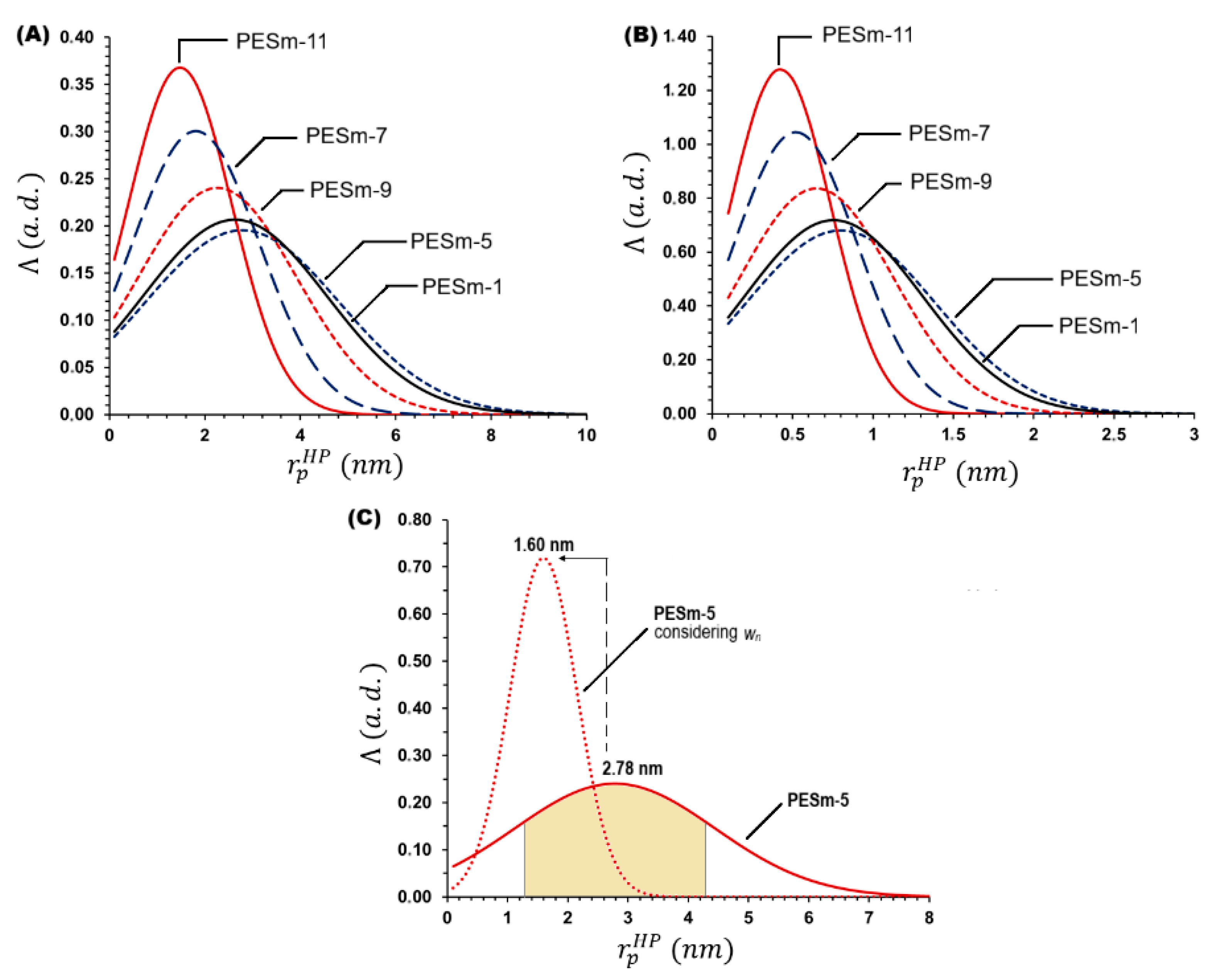
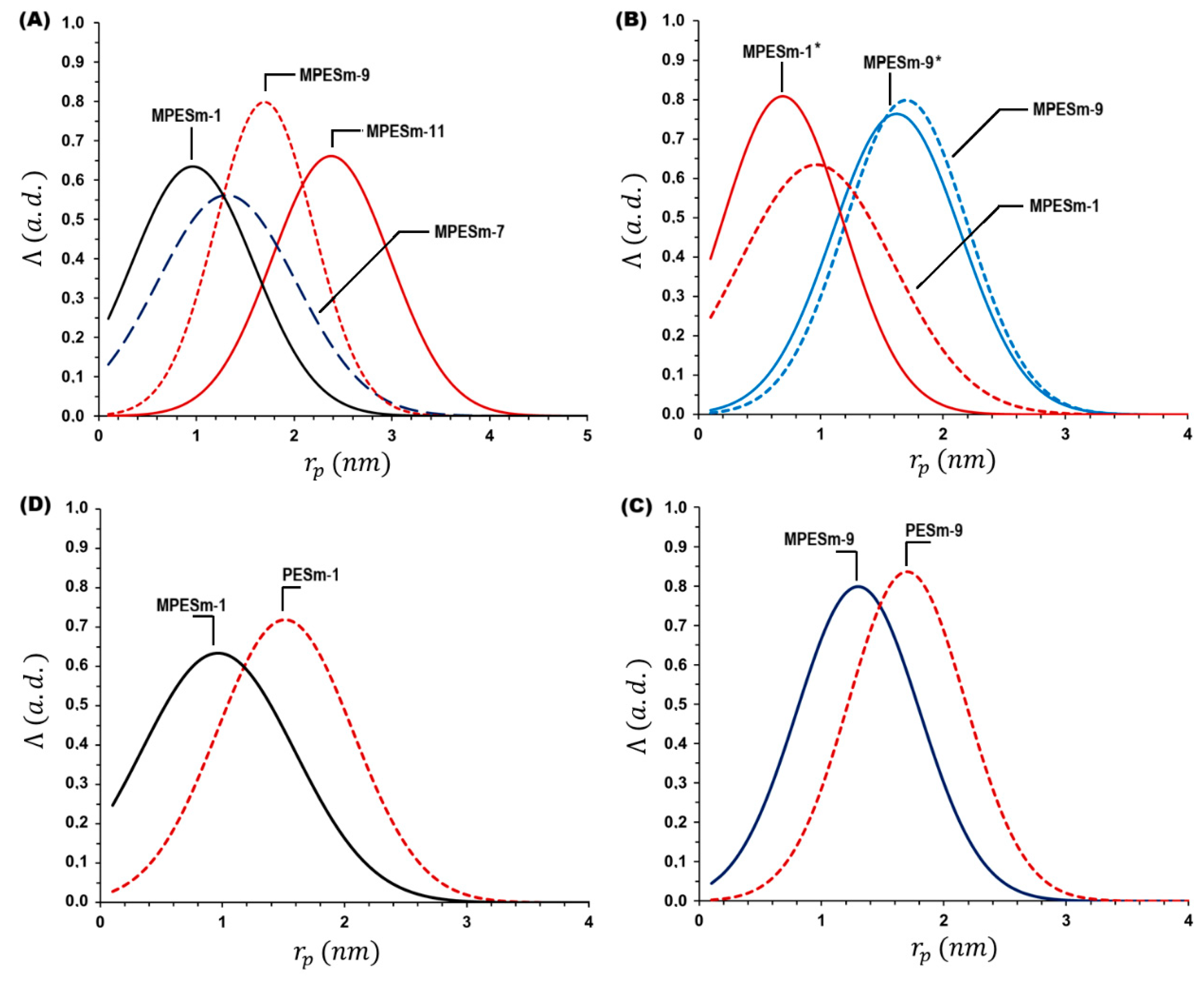
From the results shown in Table 8, pore size distribution can be simulated in different ways: (i) by assuming a normal distribution, based on the central limit theorem because n p takes very large values (see examples for five PESms in Figure 7A) and (ii) by assuming a normal distribution but assigning a weight based on n p , 1 and n p , 2 . In this case, the results show that small pores described by r p , 1 H P are much higher in number compared with the large pores defined by r p Y L ; thus, it is seen that the former accounts for approximately 90% (see examples for five PESms in Figure 7B). A comparison of the effect of applying these weights is shown in Figure 7C. Clearly, distribution is shifted toward smaller pore size values.

4.3. Structural Characteristics of Modified PESms

Darcy’s Curve Modeling for Linear and Nonlinear Regimes

Darcy’s curve simulation was based on (14); thus, this modeling allows us to establish the linear regime parameters necessary for characterizing the porous structure using information from the nonlinear regime. Note that in these experiments, because of the modification of membranes with PVA, in all cases, a loss of linearity was observed.
The loss of linearity can be attributed to different factors or a combination thereof. The first factor is the accumulation of solutes on the membrane surface. Note that as the flow rate increases, solute accumulation does not necessarily increase linearly; consequently, the relationship given by (14) is no longer proportional. However, considering that the membrane was modified with PVA, the swelling of the polymer may also play a role in nonlinearity. This phenomenon is related to a second factor. The high hydrophilicity of PVA and its macromolecular nature promotes gel formation; therefore, permeability is no longer constant, since at higher pressures, the density of the gel formed will be greater (i.e., the fouling formed is not rigid). Another aspect that cannot be overlooked is the fact that the linearity predicted by Darcy’s law is fulfilled under laminar flow, which is not necessarily maintained with the increase in pressure and the deposition of PVA both inside and on the surface of the membrane.
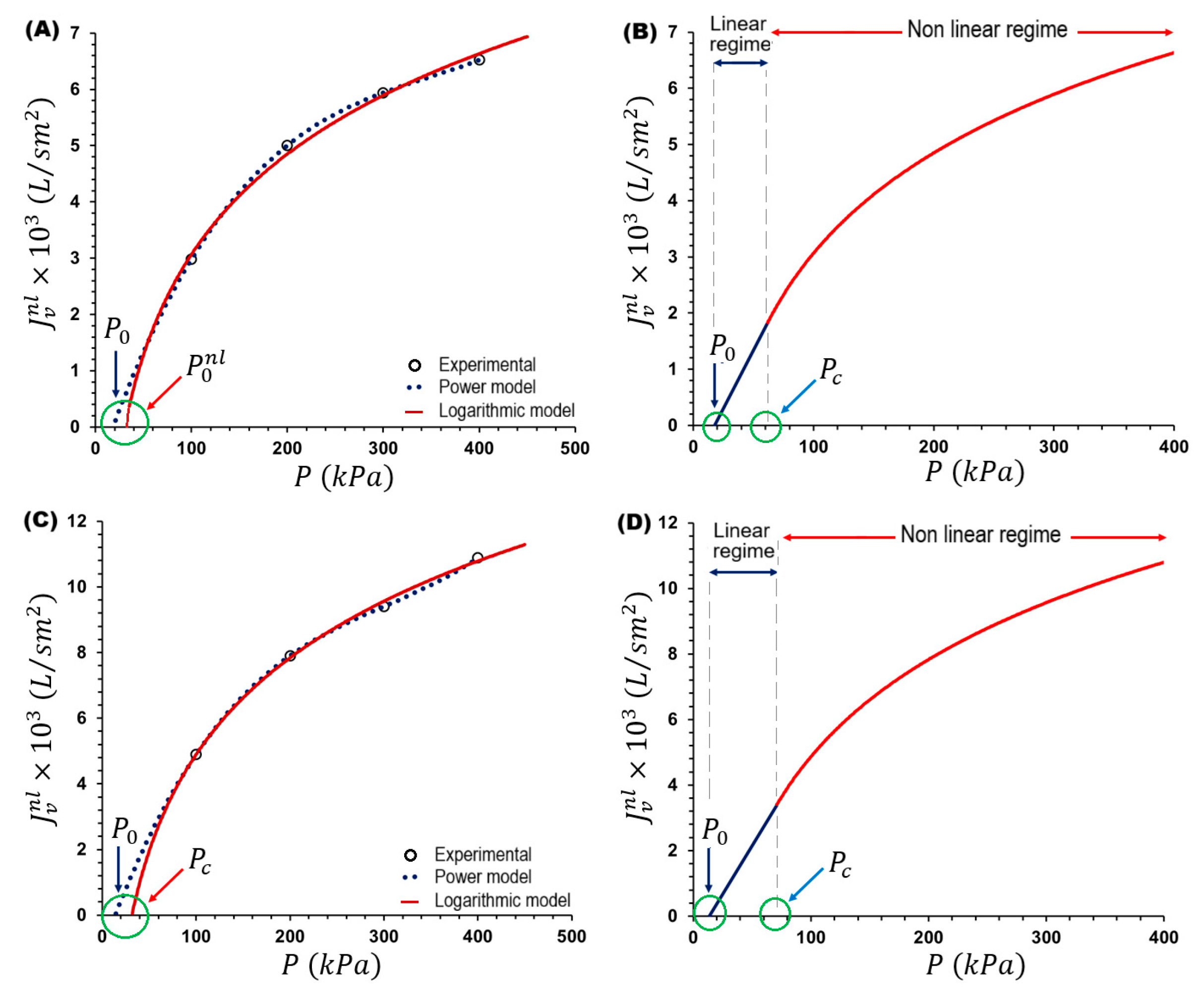
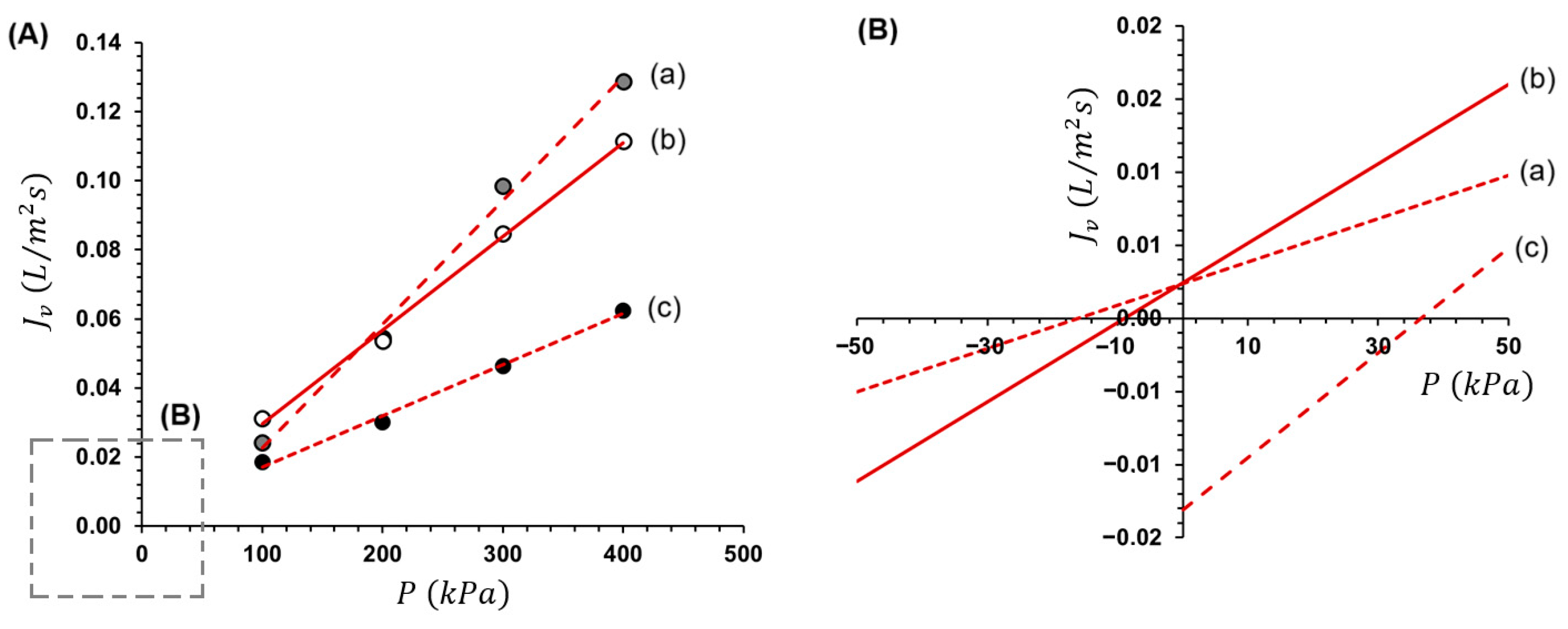
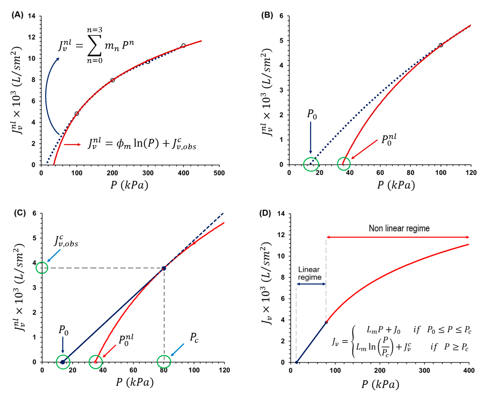
Figure 8 shows different stages of the model exemplified for one membrane. Figure 8A shows experimental data (white circles) for MPESm-1 and how these data can be fitted using two different models: an experimental power model defined by (30) and a logarithmic model, derived from (12) and (13) and shown in (14). In all cases, n = 3 in the power model; however, it might be expected that n = 3 would change for membranes with a larger pore size (e.g., microfiltration membranes). Figure 8B shows how each model is associated with two parameters: the potential model, at J v = 0 , allows us to establish P 0 , while the logarithmic model, at J v = 0 , allows us to establish P 0 n l . Figure 8C illustrates the position of P c , which is an important parameter because it allows us to differentiate between the linear and nonlinear regimes; it was seen that P c > P 0 n l > P 0 . In addition, P c is implicitly contained in both models, closely related to the maximum and minimum fluxes observed in the linear and nonlinear models, respectively. Finally, Figure 8D shows the complete simulation of Darcy’s curve for that specific membrane (MPESm-1).
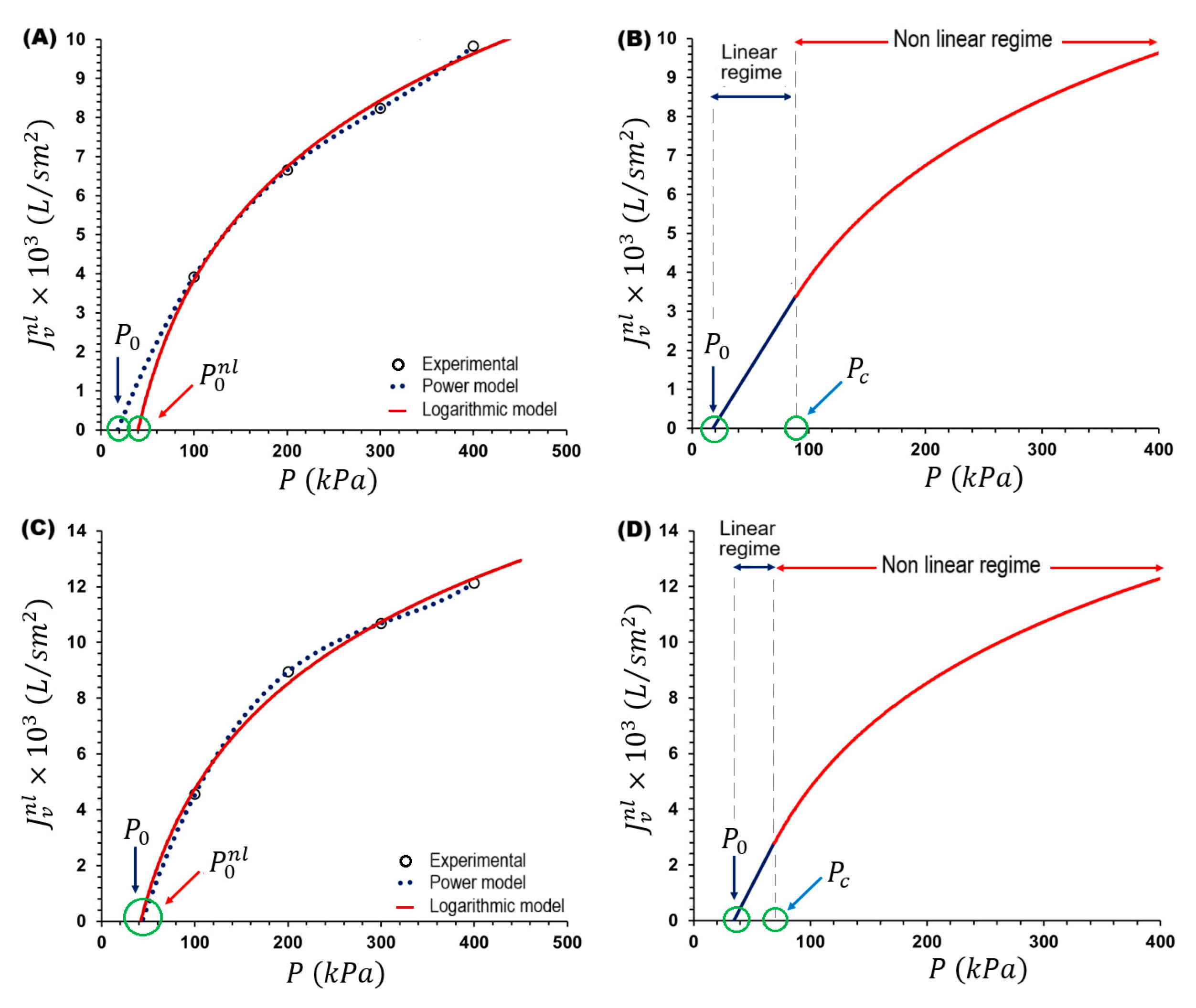
To illustrate the consistency of modeling against a wide set of PESms, J v : P plots were modeled for all modified membranes. Two examples are shown in Figure 9 and Figure 10. Note that these membranes were modified using different concentrations of PVA; therefore, different changes with respect to pristine membranes are expected. From the figures, it can be seen that the length of the linear segment ( Γ ) varies between the different membranes; therefore, it is suggested that this length is a characteristic related to porosity features.
Furthermore, for the same membrane, different relationships can be established between the different parameters, for example,
Γ 2 = P c P 0 y 2 + J v , o b s c 2
tan θ = J v , o b s c P c P 0 = J v , o b s n l P 0 n l P 0
where θ is the angle formed between the linear segment and the pressure axis, and J v , o b s n l is the flow on the linear segment corresponding to pressure P 0 n l . Note that in (34), y is introduced to achieve correct dimensional congruency (the above implies that Γ is a type of flow, but also, from the procedure approach, the graph should be re-scaled by replacing P with P / y .). Model parameters for all modified membranes are summarized in Table 9, Table 10, Table 11 and Table 12, in addition, the values of P c and J v , o b s c are shown for all membranes in Table 13.
The parameters describing the linear regimen for modified PESms are shown in Table 13. The results show that the L m and J 0 values are one order of magnitude lower than those obtained for the pristine membranes in both cases; that is, L m decreases from 10−7 to 10−8, while for J 0 , the change is from 10−3 to 10−4 (see Table 3 and Table 13). On the other hand, the P 0 values for the pristine membrane are in the range of ~3300 Pa to ~16,000 Pa, while for the modified membranes, P 0 is in the range of ~2000 to ~70,000 Pa. This suggests that although phenomena such as pore blockage may have occurred, since P 0 increased appreciably in some cases, another phenomenon directed the changes toward an increase in L m . In this regard, the polymer’s hydrophilicity suggests that the membrane became sufficiently hydrophilic in some cases to decrease flow resistance, whereas in others, pore clogging increased resistance. Consequently, both processes can occur (blocking and hydrophilicity). Furthermore, no specific behavior was identified in relation to PVA concentrations.
With the backward-scaling method and P 0 , the values of r p Y L , ε , and n p were calculated according to the procedure previously described in the methodology. However, since there was no predefined criterion for calibrating the threshold and membranes were modified by using PVA, the information used for pristine membranes is not necessarily adequate. Thus, in (21) and (22), s n was varied by changing n from 1 to 3 . As a result of this procedure, a set of values were obtained for each membrane in function of n . Because r p Y L defines the maximum pore size related to L m , a first criterion to establish the correct value is that r p Y L > r p H P . On the other hand, since r p Y L satisfies (20), the L m calculated from (22) and using r p H P must be consistent with the L m obtained from the experimental data. Thus, by comparing L m (Table 13) with the L m obtained from (202), it was possible to determine r p H P . In addition, from this procedure, it was observed that L m (in Table 13) < L m (from r p H P ), which is interpreted as a partial contribution of r p H P to the total value of L m . Results are summarized in Table 14, and a comparison between pore size distribution functions of pristine and modified membranes is shown in Figure 11.
For PES membranes, L m depends on the pore size (described by r p ), n p , and ε , while for MPESms, in addition to the aforementioned parameters, fouling will also have an influence, which is a function of the PVA concentration during filtration and the relative size of PVA chains with respect to the pore size (the smaller the difference between r g and r p is, the greater the fouling expected inside the membrane pores is). Thus, for example, the increase in L m when the PVA solution concentration is increased from 60 to 80 mmol/L reflects a decrease in r p but also an increase in ε and n p . However, it should be noted that the variability of the results is highly dependent on the accuracy of measurements during hydraulic permeability tests and the membrane’s inherent variability; therefore, a clearly defined behavior cannot be expected from the entire membrane assembly. One case that reflects the above is MPESm-10 (see Table 14), which has L m = 12.060 × 10 8 s/m, a relatively smaller r p (0.93 nm), and a high n p (i.e., high ε ) compared, for example, with MPESm-11. However, PESm-10 shows the highest r p Y L , which is almost double the r p Y L obtained for PESm-11 (see Table 8).
Figure 11A shows that membranes can be distinguished from one another by the mean value, as well as by the intensity and width of the distribution. In contrast, Figure 11B compares two modified membranes with and without taking into consideration the weight (here, weight is given by the relative contribution fraction of the different r p to L m ). The results show that while the difference is not significant for MPESm-9, it is significant for MPESm-1. Furthermore, the rightward shift in the distribution suggests that L m , in both cases, is controlled by a larger pore size fraction. Finally, Figure 11D,E illustrate the comparison of two membranes before and after modification. In both examples, the modification leads to a reduction in r p , with variations different in each case.

5. Remarks and Conclusions

This document presents the development of a model based on the HPEM concept, which is derived from the Young–Laplace equation, Darcy’s law, and the Hagen–Poiseuille permeability equation. The initial strategy supporting the model is not new, and one of the main disadvantages usually mentioned in this type of model is the need to assume geometric aspects to simplify the pore shape and the obtaining of a single-value result, which is usually referred to as an effective value. However, it should be noted that the membrane modeling approach using permeability, porosity, and flow laws allows one to describe properties that cannot be obtained by other techniques, particularly those related to real operating conditions. Furthermore, compared with traditional techniques such as SEM and mercury porosimetry, this analytical approach avoids the use of solvents and reagents (a valuable aspect from a green analytical chemistry perspective), reduces equipment and personnel costs, and enables the study of a membrane without its destruction; but also, the behavior of membranes can be studied under real operation conditions, including hydration, ionic strength, and fluids of different nature characterized by a polarity, viscosity, or surface tension different from that of water. This is particularly valuable in studies about the changes that membrane undergo due to fouling or because of controlled modifications aimed at altering or improving their properties.
On the other hand, while the use of permeability, porosity, and flow laws for modeling porous structures may initially seem unoriginal, the approach developed here is. Firstly, the difficulties inherent in the ε r p 2 product (or n p r p 4 , if preferred) result from a natural partitioning of the r p concept due to two well-established principles. Accordingly, the concepts of r p Y L (derived from the Young–Laplace capillarity equation) and r p H P (derived from the HP permeability equation) are introduced, and considering the definition of ε , the concept of r p g is also introduced. Note that the geometric mean appears naturally from the recognition that two radii derived from different physical laws exert different effects on membrane properties. Thus, although these radii can be numerically equivalent, they do not necessarily have to be. In this way, our results show that when r p Y L is consistent with surface porosity, r p H P is consistent with permeability, and vice versa. On the other hand, the introduction of two radii leads to a specific mathematical procedure that, considering only a single radius, is meaningless. The fact that two radii are defined in (17), instead of only one, allows for the separation of variables to obtain r p H P , while r p Y L is assumed as a known value. If this is not performed, the result is that the magnitude of the radius’s contribution corresponds to the fourth power, leading to drastic changes in the order of magnitude of the variables.
The proposed model is based on the premise that the void space within the membrane, which contributes to its permeability properties, can be molded into a shape without losing its spatial characteristics, since though these characteristics are distorted by the change in shape, the associated total space remains unchanged. This should be understood as follows: changes in the total pore volume can be distributed across a finite number of pores with a maximum size, in a manner consistent with the hydraulic permeability measurements. Thus, once this value is established, the analytical problem consists of finding n p , r p , and ε , which are parameters that should be compatible with the membrane’s characteristics. To achieve this, prior information is needed to calibrate the thresholds within which the results will be measured, but also, scaling corrections are needed. This procedure is supported in (2) and information obtained from the literature. Although calibration using thresholds and scaling factors may appear to be a disadvantage, it is a common strategy that allows us to correlate the results with those obtained by other techniques.
One feature of the model is the introduction of scaling factors, which depend on the available information and the results obtained. To visualize the scope of the results appropriately, greater clarity on these scaling factors should be given. Thus, the model proposed here is based on the following premises: the values taken of the model parameters must (i) satisfy a set of interrelated equations, (ii) be consistent with other analytical techniques, and (iii) agree with experimental measurements of hydraulic permeability. Since the calculation equations are not new, the novelty lies in the calculation strategy employed, which, if preferred, can be considered a calculation algorithm based on solving a system of equations using iterative numerical methods. Consequently, the scale factors are themselves iterations of the calculation rather than physical parameters of the model (in other words, they are adjustment variables).
The relationship among the four main parameters ( ε , n p , r p , and r m ) is introduced in (3). In particular, whereas r m is known from direct measurements, ε is determined from its fractional definition, such that 0 < ε < 1 . Consequently, if ε > 1 is obtained from physical equations, then an overestimation of ε is concluded, and the need of one adjustment parameter to achieve a congruent result is evident ( s ε ). Thus, by backward-scaling, the subsequent numerical problem is to find the value of s ε . Observing the results, s ε is easily defined. The strategy described here assumes that overestimation does not occur in its numerical value but in the magnitude of its scale; consequently, with s ε , only the scale is modified. Essentially, this corresponds to the value by which s ε must be multiplied for the result to be consistent with its fractional definition. However, by backward-scaling, r p Y L is calibrated, or re-scaled if preferred, using known information which can be obtained by any other technique (here, SEM from previous publications was used). Thus, the magnitude of r p Y L changes from micrometer to nanometer. Due to changes in r p Y L , s ε changes to 10−4 or 10−5 since its values must be consistent with (3) and its fractional definition. The above is explained by the interdependence of variables.
In addition, the model assumes cylindrical pores as a strategy for establishing equivalent porosity. That is, regardless of the pore shape, the membrane’s volumetric porosity remains unchanged. Note that strictly speaking, it is the surface porosity that is affected by the restriction of a cylindrical shape. However, the model does not address the membrane’s internal structure. We believe that tortuosity is a first approximation (with the simplest being the increase in the mean path length relative to the active layer thickness, assuming a cylindrical pore shape). However, the internal structure in terms of pore shape has not yet been incorporated into the model. Preliminary analyses allow us to conclude that the internal structure must be pre-defined in terms of shape categories (gaps formed by fibers, tubular bifurcations, etc.); thus, specific tortuosity models must be constructed for each category.
Finally, as shown in the results, values for n p , r p , and ε , as well as r p Y L and r p H P , were consistently established; in addition, it is demonstrated that it is possible to construct simple distribution models that facilitate the easy description of changes occurring in the membrane. This work also developed a strategy for simulating Darcy’s curve beyond the linear regime. This allows for the definition of, among other things, critical values and characteristic shapes (from models and modeling parameters), which make it possible to apply the model even when changes experienced by the membrane cause flow behavior outside the linear range. Likewise, this procedure allowed us to establish the linear range, which is useful for redirecting experiments both at the operational level and in terms of the nature of the changes. In addition, in the field of simulation and computational analysis, the model is easily programmable and adaptable to scenario planning.
Regarding the results of the PESm and MPESm study, it can be concluded that these membranes exhibit significant variability in their porous structure. Therefore, the results obtained from the average values of different membranes, based on a small sample, can have such high variation that the effects of a modification process can be easily masked, or the overall behavior of the results becomes erratic and difficult to reproduce.

Supplementary Materials

The following supporting information can be downloaded at: https://www.mdpi.com/article/10.3390/surfaces9010005/s1, Table S1: Experimental data for PESms and MPESms.

Author Contributions

Conceptualization, M.P., J.M.M.-L., J.M.D., J.S.L.V., and E.M.C.; methodology, J.M.M.-L., J.M.D., M.P., J.M.M.-L., J.M.D., J.S.L.V., and E.M.C.; investigation, data curation, writing—review and editing, and supervision, M.P.; project administration, M.P. and E.M.C.; funding acquisition, M.P. and J.M.M.-L. All authors have read and agreed to the published version of the manuscript.

Funding

This research study was funded by GENERAL ROYALTIES’ SYSTEM OF COLOMBIA (SGR/DNP/Mindtech), grant number BPIN 2020000100261; MINISTRY OF SCIENCE, TECHNOLOGY AND INNOVATION OF COLOMBIA (Minciencias), grant number C.I. 71320; and UNIVERSIDAD DE CÓRDOBA, UNIVERSIDAD DEL VALLE and MINDTECH S.A.S., grant number MT-012025, C.I. 71408 (agreement MT-AFICAT-202501).

Institutional Review Board Statement

Not applicable.

Informed Consent Statement

Not applicable.

Data Availability Statement

The main data are provided in the Supplementary Materials (Table S1) of this document.

Acknowledgments

The authors thank Eng. J.F. Benítez Cancimance and Eng. L.C. Lemos Vidarte for the data provided within the framework of their degree work related specifically to hydraulic permeability tests.

Conflicts of Interest

Jina M. Martínez-Lara and Jorge M. Durango were employed by Mindtech Research Group. The remaining authors declare that the research was conducted in the absence of any commercial or financial relationships that could be construed as a potential conflict of interest. The funders had no role in the design of the study; in the collection, analyses, or interpretation of data; in the writing of the manuscript; or in the decision to publish the results.

Abbreviations

The following abbreviations are used in this manuscript:
Latin symbols
A m Membrane   area   ( m 2 )
A p n e t Total   surface   area   of   pores   ( m 2 )
F ϵ Generating function of random error (dimensionless)
f ϵ Magnitude   of   random   error   defined   by   F ϵ (dimensionless)
J 0 Minimum   flux   ( L m 2 s 1 )
J v Volumetric   flux   ( L m 2 s 1 )
J v c Critical   volumetric   flux   ( L m 2 s 1 )
J v , o b s c Observed   critic   volumetric   flux   ( L m 2 s 1 )
J v n l Nonlinear   volumetric   flux   ( L m 2 s 1 )
L m Hydraulic   permeability   ( s m 1 )
n p Number of pores (dimensionless)
m n Coefficients of logarithmic and power models (depending on model)
n p 0 First   approximation   of   n p (dimensionless)
n p , l Lower   limit   of   n p (dimensionless)
n p , u Upper   limit   of   n p (dimensionless)
P Pressure   ( P a )
P c Critical   pressure   ( P a )
P 0 Minimum   pressure   ( P a )
P 0 * Correction   of   P 0   based   on   r p Y L   and   ε (Pa)
P 0 n l Non-lineal minimum pressure ( P a )
r m Membrane   radius   ( m )
r p Effective   mean   pore   radius   ( m )
r p ¯ Average   resulting   from   r p , 1   and   r p , 2   ( m )
r p , 1 Redefining   of   r p , l H P   ( m )
r p , 2 Redefining   of   r p , u H P   ( m )
r p Y L Young Laplace   pore   radius   ( m )
r p H P Hagen Poiseuille   pore   radius   ( m )
r p , l H P Lower   limit   of   r p H P   ( m )
r p , u H P Upper   limit   of   r p H P   ( m )
r p g Geometric   pore   radius   ( m )
s ε Scaling factor of surface porosity (dimensionless)
s n Scaling factor of pore number (dimensionless)
m Exponent   defining   s n (dimensionless)
n Variation   on   m (dimensionless)
t Time   ( s )
V m Membrane   volume   ( m 3 )
V p n e t Total   volume   of   pore   ( m 3 )
x Any independent variable (depending on variable)
y Any dependent variable (depending on variable)
y p Effective   pore   path   ( m )
w Mass   ( k g )
Greek symbols
α Constant   related   to   ε / n p   vs .   r p Y L   ( m 1 )
δ p Pore   density   ( m 2 )
ϵ n Relative random error (dimensionless)
ϵ m a x Maximum error threshold (%)
ϵ m i n Maximum error threshold (%)
ϵ m s d Mean square deviation (dimensionless)
ϵ r a d Relative absolute deviation (%)
ε Surface porosity (dimensionless)
ε e Experimental   ε (dimensionless)
σ r Standard   deviation   of   r p   ( m )
γ Surface   tension   ( N m 1 )
γ w Water   surface   tension   ( N m 1 )
μ Viscosity   of   fluid   ( P a s )
π 3.1416 (dimensionless)
τ Tortuosity (dimensionless)
θ Contact angle (radians)
v w Water   flux   rate   ( m 3 s 1 )
r p Percentage of pore size distribution (%)
y m Thickness   of   active   layer   ( m )
Λ Normal distribution (dimensionless)
Γ Length of linear segment in Darcy’s law (dimensionless)
Acronyms
AFMAtomic force microscopy
HPEMHagen–Poiseuille equivalent membrane
J v : ( P ) Flux-versus-pressure plot
MPESmModified poly(ether sulfone) membrane
PESmPoly(ether sulfone) membrane
PVAPoly(vinyl alcohol)
UFUltrafiltration
UFMUltrafiltration membrane
SEMScanning electron microscopy
TEMTransmission electronic microscopy

References

  1. Palencia, M.; Córdoba, A.; Vera, M. Membrane Technology and Chemistry. In Nanostructured Polymer Membranes: Volume 1: Processing and Characterization; Visakh, P.M., Olga, B.N., Eds.; Wiley: Hoboken, NJ, USA, 2016; pp. 27–54. [Google Scholar]
  2. Siddiqui, M.U.; Arif, A.F.M.; Bashmal, S. Permeability-Selectivity Analysis of Microfiltration and Ultrafiltration Membranes: Effect of Pore Size and Shape Distribution and Membrane Stretching. Membrane 2016, 6, 40. [Google Scholar] [CrossRef]
  3. Hidayati, N.; Hashimah, N.; Syazana, N.; Marpani, F.; Zaman, M.; Ming, C.; Meng, K.; Jye, W.; Fauzi, A. A Review on the Use of Membrane Technology Systems in Developing Countries. Membranes 2021, 12, 30. [Google Scholar] [CrossRef]
  4. Zhang, Y.; Gao, X.; Xiang, L.; Zhang, Y.; da Costa, J.C.D. Study on composite membranes with high selective permeance properties. J. Membr. Sci. 2010, 346, 318–326. [Google Scholar] [CrossRef]
  5. Lin, L.; Feng, C.; Lopez, R.; Coronell, O. Identifying facile and accurate methods to measure the thickness of the active layers of thin-film composite membranes—A comparison of seven characterization techniques. J. Membr. Sci. 2016, 498, 167–179. [Google Scholar] [CrossRef]
  6. Mudhoo, A.; Otero, M.; Chu, K.H. Insights into adsorbent tortuosity across aqueous adsorption systems. Particulogy 2024, 88, 71–88. [Google Scholar] [CrossRef]
  7. Fernandez-Pineada, C.; Serrano, F. A study of membrane hydraulic permeability obtained by different procedures. J. Mebrane Sci. 1984, 19, 325–332. [Google Scholar] [CrossRef]
  8. Palencia, M.; Lerma, M.; Palencia, V. Description of fouling, surface changes and heterogeneity of membranes by color-based digital image analysis. J. Membr. Sci. 2016, 510, 229–237. [Google Scholar] [CrossRef]
  9. Evans, C.E.; Noble, R.D.; Nazeri-Thompson, S.; Nazeri, B.; Koval, C.A. Role of conditioning on water uptake and hydraulic permeability of Nafion® membranes. J. Membr. Sci. 2006, 279, 521–528. [Google Scholar] [CrossRef]
  10. Xia, Q.-C.; Liu, M.-L.; Cao, X.-L.; Wang, Y.; Xing, W.; Sun, S.-P. Structure design and applications of dual-layer polymeric membranas. J. Membr. Sci. 2018, 562, 85–111. [Google Scholar] [CrossRef]
  11. Epstein, J.A.; Ramon, G.Z. Characterizing the permeability of a foulant layer under a transient applied pressure. J. Mebrane Sci. 2026, 738, 124683. [Google Scholar] [CrossRef]
  12. Palencia, M. Fundamental and Methodological Aspects of Porous Membrane Characterization by Hydrodynamic Permeability Test—A review. J. Sci. Technol. Appl. 2019, 7, 17–25. [Google Scholar] [CrossRef]
  13. Nakao, S.-I. Determination of pore size and pore size distribution: 3. Filtration membranas. J. Membr. Sci. 1994, 96, 131–165. [Google Scholar] [CrossRef]
  14. Rabiei, S.; Paterson, A.H.J. The Effect of Membrane Surface Hydrophobicity on the Performance and Water Production Cost of a Desalination Unit. Membranes 2025, 15, 63. [Google Scholar] [CrossRef]
  15. Mannaf, M.M.; Rahman, M.M.; Talukder, S.; Talukder, N.; Lee, E.S. Current Progress in Advanced Functional Membranes for Water-Pollutant Removal: A Critical Review. Membranes 2025, 15, 300. [Google Scholar] [CrossRef] [PubMed]
  16. Cheng, X.; Bae, J. Recent Advancements in Fabrication, Separation, and Purification of Hierarchically Porous Polymer Membranes and Their Applications in Next-Generation Electrochemical Energy Storage Devices. Polymers 2024, 16, 3269. [Google Scholar] [CrossRef]
  17. Li, S.; Zhang, H.; Li, S.; Wang, J.; Wang, Q.; Cheng, Z. Advances in hierarchically porous materials: Fundamentals, preparation and applications. Renew. Sustain. Energy Rev. 2024, 202, 114641. [Google Scholar] [CrossRef]
  18. Mason, E.A.; Lonsdale, H.K. Statistical-mechanical theory of membrane transport. J. Membr. Sci. 1990, 51, 1–81. [Google Scholar] [CrossRef]
  19. Rea, R.; Grazia de Angelis, M.; Giacinti, M. Models for Facilitated Transport Membranes: A Review. Membranes 2019, 9, 26. [Google Scholar] [CrossRef]
  20. Dong, Y.; Dai, X.; Zhao, L.; Xie, Z.; Zhang, J. Review of Transport Phenomena and Popular Modelling Approaches in Membrane Distillation. Membranes 2021, 11, 122. [Google Scholar] [CrossRef]
  21. Palencia, M.; Rivas, B.L.; Pereira, E.; Hernández, A.; Prádanos, P. Study of polymer–metal ion–membrane interactions in liquid-phase polymer-based retention (LPR) by continuous diafiltration. J. Membr. Sci. 2009, 336, 128–139. [Google Scholar] [CrossRef]
  22. Zydney, A.; Aimar, P.; Meireles, M.; Pimbley, J.; Belfort, G. Use of the log-normal probability density function to analyze membrane pore size distributions: Functional forms and discrepancies. J. Membr. Sci. 1994, 91, 293–298. [Google Scholar] [CrossRef]
  23. Zydney, A.L. High Performance Ultrafiltration Membranes: Pore Geometry and Charge Effects. Membr. Sci. Technol. 2011, 14, 333–352. [Google Scholar] [CrossRef]
  24. Tanis-Kanbur, M.B.; Peinador, R.I.; Calvo, J.I.; Hernández, A.; Chew, J.W. Porosimetric membrane characterization techniques: A review. J. Membr. Sci. 2021, 619, 118750. [Google Scholar] [CrossRef]
  25. Tran-Duc, T.; Phan-Thien, N.; Wang, J. A theoretical study of permeability enhancement for ultrafiltration ceramic membranes with conical pores and slippage. Phys. Fluids 2019, 31, 22003. [Google Scholar] [CrossRef]
  26. Tung, K.-L.; Wang, S.; Lu, W.-M.; Pan, C.-H. In situ measurement of cake thickness distribution by a photointerrupt sensor. J. Membr. Sci. 2001, 190, 57–67. [Google Scholar] [CrossRef]
  27. Pope, J.M.; Yao, S.; Fane, A.G. Quantitative measurements of the concentration polarisation layer thickness in membrane filtration of oil-water emulsions using NMR micro-imaging. J. Membr. Sci. 1996, 118, 247–257. [Google Scholar] [CrossRef]
  28. He, J.; Arbaugh, T.; Nguyen, D.; Xian, W.; Hoek, E.M.V.; McCutcheon, J.R.; Li, Y. Molecular mechanisms of thickness-dependent water desalination in polyamide reverse-osmosis membranes. J. Membr. Sci. 2023, 674, 121498. [Google Scholar] [CrossRef]
  29. Firpo, G.; Angeli, E.; Repetto, L.; Valbusa, U. Permeability thickness dependence of polydimethylsiloxane (PDMS) membranes. J. Membr. Sci. 2015, 481, 1–8. [Google Scholar] [CrossRef]
  30. Jadav, G.; Aswal, V.K.; Bhatt, H.; Chaudhari, J.C.; Singh, P.S. Influence of film thickness on the structure and properties of PDMS membrane. J. Membr. Sci. 2021, 415–416, 624–634. [Google Scholar] [CrossRef]
  31. Zhang, X.; Wei, M.; Xu, F.; Wang, Y. Thickness-dependent ion rejection in nanopores. J. Membr. Sci. 2020, 601, 117899. [Google Scholar] [CrossRef]
  32. Holzer, L.; Marmet, P.; Fingerle-Strab, M.; Wiegmann, A.; Neumann, M.; Schmidt, V. Review of Theories and a New Classification of Tortuosity Types. In Tortuosity and Microstructure Effects in Porous Media: Classical Theories, Empirical Data and Modern Methods; Springer Series in Materials Science; Springer: Berlin/Heidelberg, Germany, 2023. [Google Scholar] [CrossRef]
  33. Holzer, L.; Marmet, P.; Fingerle-Strab, M.; Wiegmann, A.; Neumann, M.; Schmidt, V. Tortuosity-Porosity Relationships: Review of Empirical Data from Literature. In Tortuosity and Microstructure Effects in Porous Media: Classical Theories, Empirical Data and Modern Methods; Springer Series in Materials Science; Springer: Berlin/Heidelberg, Germany, 2023. [Google Scholar] [CrossRef]
  34. Griffiths, I.M.; Mitevski, I.; Vujkovac, I.; Illingworth, M.R.; Stewart, P.S. The role of tortuosity in filtration efficiency: A general network model for filtration. J. Membr. Sci. 2020, 598, 117664. [Google Scholar] [CrossRef]
  35. Alqaheem, Y.; Alomair, A.A. Microscopy and Spectroscopy Techniques for Characterization of Polymeric Membranes. Membranes 2020, 10, 33. [Google Scholar] [CrossRef]
  36. Bohr, S.J.; Wang, F.; Metze, M.; Vukusik, J.L.; Sapalidis, A.; Ulbricht, M.; Nestler, B.; Barbe, S. State-of-the-art review of porous polymer membrane formation characterization—How numerical and experimental approaches dovetail to drive innovation. Front. Sustain. 2023, 4, 1093911. [Google Scholar] [CrossRef]
  37. Kim, K.J.; Fane, A.G.; Aim, R.B.; Liu, M.G.; Jonsson, G.; Tessaro, I.C.; Broek, A.P.; Bargeman, D. A comparative study of techniques used for porous membrane characterization: Pore characterization. J. Membr. Sci. 1994, 87, 35–46. [Google Scholar] [CrossRef]
  38. Tamime, R.; Wyart, Y.; Siozade, L.; Baudin, I.; Deumie, C.; Glucina, K.; Moulin, P. Membrane Characterization by Microscopic and Scattering Methods: Multiscale Structure. Membranes 2011, 1, 91–97. [Google Scholar] [CrossRef]
  39. Masselin, I.; Durand-Bourlier, L.; Laine, J.-M.; Sizaret, P.-Y.; Chasseray, X.; Lemordant, D. Membrane characterization using microscopic image analysis. J. Membr. Sci. 2001, 186, 85–96. [Google Scholar] [CrossRef]
  40. AlMarzooqi, F.A.; Bilad, M.R.; Mansoor, B.; Arafat, H.A. A comparative study of image analysis and porometry techniques for characterization of porous membranes. J. Mater. Sci. 2016, 51, 2017–2032. [Google Scholar] [CrossRef]
  41. Luo, J.; Wan, Y. Effects of pH and salt on nanofiltration—A critical review. J. Membr. Sci. 2013, 438, 18–28. [Google Scholar] [CrossRef]
  42. Fane, A.G.; Fell, C.J.D.; Waters, A.G. The relationship between membrane surface pore characteristics and flux for ultrafiltration membranas. J. Membr. Sci. 1981, 9, 245–262. [Google Scholar] [CrossRef]
  43. Pusch, W.; Walch, A. Membrane structure and its correlation with membrane permeability. J. Membr. Sci. 1982, 10, 325–360. [Google Scholar] [CrossRef]
  44. Mondal, S.; Griffiths, I.M.; Ramon, G.Z. Forefronts in structure–performance models of separation membranas. J. Membr. Sci. 2019, 588, 117166. [Google Scholar] [CrossRef]
  45. Santisukkasaem, U.; Olawuyi, F.; Oye, P.; Diganta, B.D. Artificial Neural Network (ANN) For Evaluating Permeability Decline in Permeable Reactive Barrier (PRB). Environ. Process 2015, 2, 291–307. [Google Scholar] [CrossRef]
  46. Hasnaoui, H.; Krea, M.; Roizard, D. Neural networks for the prediction of polymer permeability to gases. J. Membr. Sci. 2017, 541, 541–549. [Google Scholar] [CrossRef]
  47. Bestwick, T.; Beckmann, J.; Camarda, K.V. Using Artificial Neural Networks to Predict Physical Properties of Membrane Polymers. Chem. Ing. Tech. 2022, 95, 363–367. [Google Scholar] [CrossRef]
  48. Zhao, Y.; Altschuh, P.; Santoki, J.; Griem, L.; Tosato, G.; Selzer, M.; Koeppe, A.; Nestler, B. Characterization of porous membranes using artificial neural networks. Acta Mater. 2023, 253, 118922. [Google Scholar] [CrossRef]
  49. Quezada, C.; Estay, H.; Cassano, A.; Troncoso, E.; Ruby-Figueroa, R. Prediction of Permeate Flux in Ultrafiltration Processes: A Review of Modeling Approaches. Membranes 2011, 11, 368. [Google Scholar] [CrossRef] [PubMed]
  50. Espinosa-Duque, A.; Mora, M.A.; Palencia, M. Modeling of constant-volume continuous diafiltration by solute distribution space’s perturbations through geometric series: Part I: Inert system (Washing method). J. Sci. Technol. Appl. 2021, 11, 13–23. [Google Scholar] [CrossRef]
  51. Nist. Nist Chemistry Web Book (Revised 2025). Available online: https://webbook.nist.gov/chemistry/fluid/ (accessed on 30 October 2025).
  52. Otitoju, T.A.; Ahmad, A.L.; Ooi, B.S. Recent advances in hydrophilic modification and performance of polyethersulfone (PES) membrane via additive blending. RSC Adv. 2018, 8, 22710–22728. [Google Scholar] [CrossRef]
  53. Pons, M.-N.; Dodds, J. Chapter Fifteen—Particle Shape Characterization by Image Analysis. In Progress in Filtration and Separation; Academic Press: New York, NY, USA, 2015; pp. 609–636. [Google Scholar] [CrossRef]
  54. Jia, X.; Garboczi, E. Advances in shape measurement in the digital world. Particuology 2016, 26, 19–31. [Google Scholar] [CrossRef]
Figure 1. Dead-end UF system used for hydraulic permeability test and surface membrane modification.
Surfaces 09 00005 g001
Figure 2. (A) Examples of hydraulic permeability test on three PESms (from 100 to 500 kPa; PESms with molecular weight cut-off of 10 kDa). (B) Magnification of zone named “B” shown in (A) is the projection of linear correlation models: (a) PESm-5, (b) PESm-8, and (c) PESm-11.
Surfaces 09 00005 g002
Figure 3. (A) Example of J v : P plot simulated based on (22) and (23) with ϵ m a x = 5 % : (a) experimental data and (b) simulated data. (B) and (C) show values of twenty random events separately obtained for determining ϵ r a d , ϵ m s d , ϵ r a d m a x , and ϵ m s d m a x of P (maximum value in grey).
Surfaces 09 00005 g003
Figure 4. Illustration of how the model achieves the result: the permeability features of the real membrane are used to describe the permeability features of the HPEM; later, by re-scaling, model changes the values of n p and r p H P , maintaining ε constant. As selection criterium, r p , l H P r p H P r p , u H P is used.
Surfaces 09 00005 g004
Figure 5. J v : P plots for all membranes, from PESm-1 to PESm-12.
Surfaces 09 00005 g005
Figure 6. Behavior of data for all PESms in this study: (A) ε / n p in function of r p Y L : (a) n p , 2 and (b) n p , 1 . (B) ε / n p 0.5 in function of r p Y L : (a) n p , 2 and (b) n p , 1 .
Surfaces 09 00005 g006
Figure 7. Pore size distribution simulated from model: (A) Examples of PESms without taking in consideration n p . (B) Examples of PESm considering n p to define the weight ( w n ). (C) Illustration of effect of the defining of w n on distribution.
Surfaces 09 00005 g007
Figure 8. Description of parameters related to Darcy’s curve and its modeling: (A) Empirical power model ( n = 3 ) (dotted line) and logarithmic model (red line). Experimental data are shown as white circles. (B) Identification of P 0 and P 0 n l from different models (power and logarithmic models, respectively). (C) Determination of P c from tangent line to logarithmic model which contains P 0 . (D) Darcy’s curve modeling for MPESm-1.
Surfaces 09 00005 g008
Figure 9. Modeling of MPESms with PVA: Fits of experimental data with (14) and (30) for MPESm-2 and MPESm-5 are shown in (A) and (C), respectively, while their corresponding Darcy’s curves are shown in (B) and (D), respectively.
Surfaces 09 00005 g009
Figure 10. Modeling of MPESms with PVA: Fits of experimental data with (14) and (30) for MPESm-8 and MPESm-11 are shown in (A) and (C), respectively, while their corresponding Darcy’s curves are shown in (B) and (D), respectively.
Surfaces 09 00005 g010
Figure 11. Modeling of pore size distribution for MPESms. (A) Example of distribution obtained for four membranes using, as statistical weight, the contribution relative to L m . (B) Exemplification of effect of considering the statistical weight on the distribution (* denotes curves for which statistical weight is not considered). (C) and (D) show a comparison of two distributions before and after modification with PVA.
Surfaces 09 00005 g011
Table 1. Methods for determining membrane structural parameters [7,11,13,24,26,27,33,40].
ParameterMethodComments
Effective pore sizeMercury
porosimetry
It can cover a wide range of pore sizes (from nm to μm). The membrane must be ruptured to perform the analysis; mercury, which is toxic, is used; the method does not distinguish between connected and closed pores; and high pressure may compress the material. It is not directly applicable in situ; therefore, it does not offer any information about the membrane in operation.
Relative
permeability method
This method is non-destructive and applicable to dry or wet membranes. It requires assumptions about pore geometry (cylindrical and straight), makes it difficult to separate parallel effects of pores of different sizes, is affected by gas/liquid adsorption effect, and in liquids, permeation can be in a nonlinear regime due to polarization or saturation.
Electron
microscopy (SEM/TEM) in combination with image analysis
This technique provides direct visual information and allows for the analysis of size distribution, morphology, and irregular shapes. In SEM, membrane collapse or structural change during pretreatment (coating with gold) may occur. Observation is limited to the surface (it does not provide information on pore depth), small pores may not be visible, and image segmentation is subjective. Moreover, it does not provide information on membrane behavior during operation.
Atomic force
microscopy (AFM) by tipping
The dimensions of open pores on the surface can be estimated. However, this technique presents difficulties like those of SEM analysis, and the scan is slow and covers a small area. It does not provide information about membrane behavior during operation.
Surface
porosity and
number of pores
Mass
measurement of accessible pore volume
For a known liquid density, the surface pore volume is obtained. Liquid may not penetrate all pores (due to meniscus effects), and surface retention, weighing error, and inability to distinguish closed pores are possible.
Microscopy combined with pore counting
using image analysis
From SEM micrographs, visible pores in a known area can be counted, and using their diameters, the pore density (number/area) can be calculated. However, this approach is subject to sampling bias and failure to count small pores, does not account for small undetectable pores, neglects depth effects, and represents a 2D projection of a 3D structure. It does not provide information about membrane behavior during operation.
Flow porosimetry (using gas/liquid permeation)Assuming that each pore behaves as a capillary, permeation can be estimated from the number of effective pores contributing to the total flow. By knowing the flow rate, the mean pore diameter, and the tortuosity, the number of active pores can be inferred. However, this method requires a geometric model and assumptions of uniformity and can overestimate “ghost” pores that are not actually permeable.
TortuosityDiffusion of
tracers in the pore
The effective diffusion of a solute through the pore is measured and compared with its diffusion in free solution. However, solute interaction with the pore wall, absorption, local diffusion in boundary layers, internal concentration gradients, and crossflow conditions may alter the diffusion of tracers.
3D tomography imagesThis technique allows for the reconstruction of the 3D internal structure of membranes with adequate resolution, the plotting of simulated flow paths (Monte Carlo line method), and the calculation of the average true length relative to geometric length (thickness). However, it offers limited resolution for nanometer-sized pores and insufficient contrast between the polymer phase and void, and it requires long processing times. In addition, artifacts may arise during volume reconstruction and segmentation of 3D data.
Empirical
modeling using hydraulic
permeability and porosity data
A porous medium-type relationship must be assumed (e.g., modified Kozeny–Carman equation). This approach uses simplified models that assume uniform, cylindrical pores without confluence, neglects edge effects, and is sensitive to errors in various parameters.
Active layer
thickness
Cross-section
microscopy (SEM)
The method requires preparing a cross-section of the membrane (e.g., by freeze-fracture and ultramicrotomy), after which the thickness of the active layer is measured from SEM micrographs. However, local damage or deformation may occur during sectioning, and membrane layers may be indistinguishable because of low contrast or inadequate sample alignment.
Tracer penetration profiling
(diffusion
labeling)
This approach requires introducing a labeled solute (fluorescent or radiolabeled) on one side and monitoring its penetration depth over a controlled time frame. The maximum useful penetration depth is then taken as an estimate of the active layer thickness. However, inhomogeneous diffusion, drag effects, wall interactions, concentration gradients, and insufficient diffusion time may occur.
Methods based on acoustic or
ellipsometrical
responses
For thin membranes, ellipsometry or other optical techniques can be used to measure thin-layer thickness. These methods require optically flat membranes, knowledge of the refractive index, sufficient contrast, and proper calibration, and they are not always suitable for thick porous membranes.
Table 2. Parameters of PESms.
ParameterSymbolUnitValueTechniqueRef.
Effective area A m m 2 0.0034Direct[45]
Effective pore radius r p n m 3.15 ± 0.25 Solute retention test[45]
Active layer thickness y m 1.075 × 10 4 SEM[45]
Number of pores n p - 7.55 × 10 9 SEM[45]
Surface mean pore radius r p μ m 140.0   ± 0.31 SEM[45]
Contact angle (H2O/PESm) θ w ° 75.6 Sessile drop[46]
Water viscosity (25 °C) μ P a s 0.891Database[51]
Water flux rate (25 °C) J w m 3 s 1 9.578 × 10 8 Calculated -
Table 3. Linear models and P 0 for all PESms included in this work.
ID L m × 10 7 ( s m 1 ) J 0 × 10 3 ( L m 2 s 1 ) r 2 ( n . d . ) P 0 ( P a )
PESm-12.712.430.99658964.5
PESm-22.593.130.996812,086.3
PESm-32.811.310.99624671.0
PESm-43.231.070.99723300.1
PESm-53.272.770.99748472.3
PESm-63.253.150.99749675.2
PESm-72.731.120.94954121.3
PESm-83.581.310.99433649.0
PESm-93.531.170.99923299.0
PESm-101.871.320.99067045.9
PESm-111.492.370.994415,958.3
PESm-121.412.120.987215,055.1
x ¯ 2.711.940.99108024.8
s 0.750.810.01364511.8
C V   ( % ) 27.841.861.370056.22
ID (identification); r 2 (linear correlation coefficient); x ¯ (mean value); s (standard deviation); C V   ( % ) (coefficient of variation); n.d. (no dimension).
Table 4. Simulation results of random error in determining L m .
Error ϵ m a x ( % ) P ( k P a ) t ( s ) w ( k g )
ϵ ¯ o b s ϵ o b s m a x ϵ ¯ o b s ϵ o b s m a x ϵ ¯ o b s ϵ o b s m a x
ϵ r a d ( % ) 54.88.30.070.20.350.85
20.92.90.040.10.470.97
10.41.80.020.040.340.81
ϵ m s d   ( n . d . ) 55.410.737.03.4439.319.1
22.83.757.90.9306.120.1
10.61.733.20.90191724.3
n.d. (no dimension).
Table 5. Simulation results of random error in determining P 0 .
Error ϵ m a x ( % ) P ( k P a ) t ( s ) w ( k g )
ϵ ¯ o b s ϵ o b s m a x ϵ ¯ o b s ϵ o b s m a x ϵ ¯ o b s ϵ o b s m a x
ϵ r a d ( % ) 548.093.12.15.320.753.5
212.627.04.442.715.744.1
17.818.20.450.911.637.2
ϵ m s d   ( n . d . ) 52.65.5108.2279.165.613013.2
20.72.346.2109.32424.82638
10.151.21.5359.45132496.1
n.d. (no dimension).
Table 6. Results of porous structure characterization for three PESms by forward-scaling method.
ParameterMembrane
PESm-1PESm-2PESm-3
Young Laplace   r p r p Y L ( μ m ) 3.992.967.66
Surface porosity ε (n.d.)13.022.736.0
Scaling   factor   for   ε s ε (n.d.)101101101
Hagen Poiseuille   r p (first approx.) r p , 0 H P ( μ m ) 1.260.940.77
Number of pores (first approx.) n p 0 × 10 6 (n.d.)8.8527.956.74
Scaling   factor   for   n p for lower limit s n (n.d.)107106107
Lower   limit   of   n p n p , l × 10 13 (n.d.)8.852.796.74
Lower   limit   of   r p H P r p , l H P ( n m ) 1.262.962.42
Scaling   factor   for   n p for upper limit s n (n.d.)106105106
Upper   limit   of   n p n p , u × 10 12 (n.d.)8.852.796.74
Upper   limit   of   r p H P r p , u H P ( n m ) 3.999.377.66
Width of pore size distribution r p ( n m ) 2.736.415.24
Mean   r p H P r p ¯ ( n m ) 1.37 ± 1.933.21 ± 4.532.62 ± 3.71
Surface mean pore radius r p ( μ m ) 98.6130.1189.3
Standard   deviation   of   r p σ r ( n m ) ±39.1±51.5±75.0
n.d. (no dimension).
Table 7. Results of porous structure characterization for three PESms by backward-scaling method.
ParameterMembrane
PESm-1PESm-2PESm-3
Young Laplace   r p r p Y L ( n m ) 3.992.967.66
Scaling   factor   for   r p Y L s Y L (n.d.)10−310−310−3
Surface porosity ε (n.d.)0.130.230.36
Scaling   factor   for   ε s ε (n.d.)10−510−510−4
Hagen Poiseuille   r p (first approx.) r p , 0 H P ( μ m ) 1.260.940.77
Number of pores (first approx.) n p 0 × 10 12 (n.d.)8.8527.956.74
Scaling   factor   for   n p for upper limit s n (n.d.)10010−1100
Upper   limit   of   n p n p , u × 10 12 (n.d.)8.853.076.74
Upper   limit   of   r p H P r p , u H P ( n m ) 3.999.377.66
Lower   limit   of   n p n p , l × 10 12 (n.d.)88.52.7967.4
Scaling   factor   for   n p for lower limit s n (n.d.)101100101
Lower   limit   of   r p H P r p , l H P ( n m ) 1.262.962.42
n.d. (no dimension).
Table 8. Results of porous structure characterization for PESms (from PESm-1 to PESm-12).
Membrane ε r p Y L n p , 1 r p , 1 H P n p , 2 r p , 2 H P r p ¯ σ r
( % ) ( μ m ) ( n . d . ) ( n m ) ( n . d . ) ( n m ) ( n m ) ( n m )
PESm-113.03.9988.51.268.83.992.631.93
PESm-222.72.9627.92.962.89.376.164.53
PESm-336.67.666.72.4267.47.665.043.71
PESm-421.010.851.93.4319.310.857.145.24
PESm-514.04.238.54.2385.013.368.796.46
PESm-618.23.7014.43.701.411.707.705.66
PESm-727.78.693.92.7539.88.695.724.20
PESm-828.59.813.23.1032.19.816.464.74
PESm-923.010.852.13.4321.110.857.145.25
PESm-1055.55.0823.31.6123.35.083.342.46
PESm-1122.62.2448.72.2448.77.094.673.43
PESm-1219.12.3836.52.3836.57.524.953.64
Surface porosity ( ε ) ; number of pores ( n p , 1 × 10 11 and n p , 2 × 10 10 ); Young–Laplace radius ( r p Y L ); lower, upper, and mean Hagen–Poiseuille radii ( r p , 1 H P , r p , 2 H P , and r p ¯ , respectively, where r p , 2 H P = r p Y L s Y L ); standard deviation of r p ¯ ( σ r ); surface mean pore radius ( r p ); n.d. (no dimension).
Table 9. Model parameters obtained from (14) and (30) for three PESms modified using 60 mmol/L PVA (MPESm-1, MPESm-2, and MPESm-3): logarithmic model (a) and power model (b).
(a) Logarithmic model:  J v n l = m 1 l n ( P ) + m 0
ParameterunitMPESm-1MPESm-2MPESm-3
P ( × 10 3 ) P a 100–400100–400100–400
m 1 ( × 10 3 ) L / s m 2 4.56194.24984.0243
m 0 ( × 10 2 ) L / s m 2 −4.7720−4.4031−4.1328
r 2 (n.d.)0.99890.99810.9987
(b) Power model:  J v n l = m 3 P 3 + m 2 P 2 + m 1 P + m 0
ParameterunitMPESm-1MPESm-2MPESm-3
m 3 ( × 10 19 ) L / s m 2 P 3 2.05172.43052.1197
m 2 ( × 10 13 ) L / s m 2 P 2 −1.9439−2.2051−1.9615
m 1 ( × 10 8 ) L / s m 2 P 7.54247.91577.2396
m 0 ( × 10 4 ) L / s m 2 −9.8046−1.0545−4.8687
r 2 (n.d.)1.00001.00001.0000
n.d. (no dimension).
Table 10. Model parameters obtained from (14) and (30) for three PESms modified using 80 mmol/L PVA (MPESm-4, MPESm-5, and MPESm-6): Logarithmic model (a) and power model (b).
(a) Logarithmic model:  J v n l = m 1 l n ( P ) + m 0
ParameterunitMPESm-4MPESm-5MPESm-6
P ( × 10 3 ) P a 100–400100–400100–400
m 1 ( × 10 3 ) L / s m 2 5.99205.44625.1940
m 0 ( × 10 2 ) L / s m 2 −6.4632−5.7950−5.5084
r 2 (n.d.)0.99810.99230.9995
(b) Power model:  J v n l = m 3 P 3 + m 2 P 2 + m 1 P + m 0
ParameterunitMPESm-4MPESm-5MPESm-6
m 3 ( × 10 19 ) L / s m 2 P 3 1.84593.95282.0589
m 2 ( × 10 13 ) L / s m 2 P 2 −2.1245−3.7015−2.1102
m 1 ( × 10 8 ) L / s m 2 P 9.49401.27338.6308
m 0 ( × 10 4 ) L / s m 2 −3.3023−4.8747−2.0570
r 2 (n.d.)1.00001.00001.0000
n.d. (no dimension).
Table 11. Model parameters obtained from (14) and (30) for three PESm modified using 100 mmol/L PVA (MPESm-7, MPESm-8, and MPESm-9).
Logarithmic model:  J v n l = m 1 l n ( P ) + m 0
ParameterunitMPESm-7MPESm-8MPESm-9
P ( × 10 3 ) P a 100–400100–400100–400
m 1 ( × 10 3 ) L / s m 2 2.74842.57312.3600
m 0 ( × 10 2 ) L / s m 2 −2.8724−2.6556−2.3870
r 2 (n.d.)0.99450.99380.9968
Power model:  J v n l = m 3 P 3 + m 2 P 2 + m 1 P + m 0
ParameterunitMPESm-7MPESm-8MPESm-9
m 3 ( × 10 19 ) L / s m 2 P 3 7.83211.21876.2268
m 2 ( × 10 13 ) L / s m 2 P 2 −9.7024−1.2731−7.7447
m 1 ( × 10 8 ) L / s m 2 P 4.45804.98673.6424
m 0 ( × 10 4 ) L / s m 2 −7.2466−8.52693.2163
r 2 (n.d.)1.00001.00001.0000
n.d. (no dimension).
Table 12. Model parameters obtained from (14) and (30) for three PESm modified using 120 mmol/L PVA (MPESm-7, MPESm-8, and MPESm-9): Logarithmic model (a) and power model (b).
(a) Logarithmic model:  J v n l = m 1 l n ( P ) + m 0
ParameterunitMPESm-10MPESm-11MPESm-12
P ( × 10 3 ) P a 100–400100–400100–400
m 1 ( × 10 3 ) L / s m 2 4.02644.33643.9303
m 0 ( × 10 2 ) L / s m 2 −4.2405−4.6148−4.1327
r 2 (n.d.)0.98270.98380.9998
(b) Power model:  J v n l = m 3 P 3 + m 2 P 2 + m 1 P + m 0
ParameterunitMPESm-10MPESm-11MPESm-12
m 3 ( × 10 19 ) L / s m 2 P 3 3.0831 1.96110.7886
m 2 ( × 10 13 ) L / s m 2 P 2 −2.8313−1.7534−0.9775
m 1 ( × 10 8 ) L / s m 2 P 9.4953 6.62045.0443
m 0 ( × 10 4 ) L / s m 2 −3.2024−1.1414−2.0558
r 2 (n.d.)1.00001.00001.0000
n.d. (no dimension).
Table 13. Parameters describing the linear regimen for modified PESms. The linear model is described by J v = L m P + J 0 with P 0 P P c .
Membrane L m J 0 P 0 P c J v , o b s c
C P V A ( s / m ) ( L / s m 2 ) ( P a ) ( P a ) ( L / s m 2 )
( m m o l / L ) × 10 8 × 10 2 × 10 3 × 10 3 × 10 3
60MPESm-15.685−7.65213.45980.03.78
MPESm-26.004−8.29013.80875.03.67
MPESm-35.643−3.8666.851075.03.85
80MPESm-47.176−2.71937.88984.03.31
MPESm-57.949−2.75534.66270.02.81
MPESm-69.404−3.56325.36855.01.61
100MPESm-73.660−6.17216.86675.02.13
MPESm-84.168−7.46217.90462.01.84
MPESm-93.414−8.2732.423475.02.48
120MPESm-1012.060−4.56137.81443.00.63
MPESm-114.725−8.54718.08989.03.35
MPESm-124.093−1.6814.107398.03.84
Table 14. Porous structure characterization of MPESms.
PVAMPESm ε r p Y L n p Y L r p H P n p H P r p ¯ ±   σ r
× 10 13 × 10 13
( m M ) ( % ) ( n m ) ( a . d . ) ( n m ) ( a . d . ) ( n m ) ( n m )
6016.02.670.92.260.92.470.29
27.02.611.12.151.12.380.32
316.00.5361.50.2861.50.400.18
80461.00.9573.10.9073.10.930.03
557.01.0456.80.3456.80.690.49
636.01.4219.30.6419.31.030.55
10076.02.131.51.441.51.790.49
88.02.012.11.282.11.640.52
912.01.485.80.705.81.090.56
1201010.00.9512.20.9112.20.930.03
119.01.992.51.252.51.620.52
1241.00.8857.60.7757.60.820.08
mM (mmol/L); n.d. (no dimension).
Disclaimer/Publisher’s Note: The statements, opinions and data contained in all publications are solely those of the individual author(s) and contributor(s) and not of MDPI and/or the editor(s). MDPI and/or the editor(s) disclaim responsibility for any injury to people or property resulting from any ideas, methods, instructions or products referred to in the content.