Bias Analysis and Correction in Weighted-L₁ Estimators for the First-Order Bifurcating Autoregressive Model

Abstract

This study examines the bias in weighted least absolute deviation ($\mathrm{W}{L}_1$) estimation within the context of stationary first-order bifurcating autoregressive (BAR(1)) models, which are frequently employed to analyze binary tree-like data, including applications in cell lineage studies. Initial findings indicate that $\mathrm{W}{L}_1$ estimators can demonstrate substantial and problematic biases, especially when small to moderate sample sizes. The autoregressive parameter and the correlation between model errors influence the volume and direction of the bias. To address this issue, we propose two bootstrap-based bias-corrected estimators for the $\mathrm{W}{L}_1$ estimator. We conduct extensive simulations to assess the performance of these bias-corrected estimators. Our empirical findings demonstrate that these estimators effectively reduce the bias inherent in $\mathrm{W}{L}_1$ estimators, with their performance being particularly pronounced at the extremes of the autoregressive parameter range.

1. Introduction

The bifurcating autoregressive (BAR) model is widely employed to analyze binary tree-structured data, as illustrated in Figure 1, which frequently arise in various applications, most notably in cell lineage studies (see, e.g., [1,2,3,4]). The BAR(1) model was initially proposed by [5] to model cell lineage data. This model extends the first-order autoregressive AR(1) model by accounting for a unique aspect: observations on two sister cells, which share the same mother cell, that are correlated. In practical settings, the BAR(1) model is useful for modeling the single-cell reproduction progress c.f. [3]. A number of studies have addressed the estimation and inference challenges associated with the BAR model (see, e.g., [5,6,7,8,9,10,11,12,13], among others).

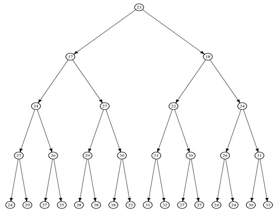
Figure 1. The lifetimes (in minutes) of E. coli cells are represented in this tree, constructed using data from [5].

Maximum likelihood (ML) estimators for the model coefficients and the correlation between errors for the BAR(1) model were introduced by [5] under the assumption of normally distributed errors. Building on this foundation, ref. [8] examined the asymptotic properties of the ML estimators for the BAR(p) model, also assuming the normality of errors. In contrast, ref. [10] explored least squares (LS) estimation for BAR(p) models without imposing distributional assumptions on the errors. In their study, they developed LS estimators for the model coefficients and introduced consistent estimators for the correlation between model errors. They further derived the asymptotic distribution of the LS estimators. However, the study did not address the finite-sample properties of these estimators. While LS estimators of BAR model coefficients are asymptotically unbiased, ref. [13] demonstrated that the finite sample bias of these estimators can be substantial, potentially leading to inaccurate inferences. This outcome is consistent with the well-known fact that LS estimators for the AR(1) model often exhibit significant bias, especially when the autoregressive parameter is near its limitations ($\pm 1$) (e.g., [14]).

To address this issue, ref. [13] introduced two bias correction techniques for the LS estimator of the autoregressive parameter in the BAR(1) model: one based on asymptotic linear bias functions and another using a bootstrapping approach. Their results indicated that both methods effectively reduce the bias, with the bootstrap bias-correction method proving more efficient than the asymptotic linear bias function method, particularly when the parameter is close to the upper boundary (i.e., near $+1$).

A related challenge in analyzing cell lineage data involves handling outliers. Several approaches have been proposed to develop robust estimators that mitigate the impact of outliers within the BAR model context, including quasi-maximum likelihood estimation methods (cf., [15,16]). In this direction, ref. [12] developed robust estimators for the first-order BAR model based on weighted absolute deviations. They demonstrated that, when the weights are fixed, the resulting estimator is an $L_1$-type estimator, offering robustness against outliers in the response space and showing greater efficiency than the least squares (LS) estimator in the presence of heavy-tailed error distributions. In contrast, when the weights are random and dependent on the points in the factor space, the weighted $L_1$ ($\mathrm{W}{L}_1$) estimator shows robustness against outliers in the factor space. Additionally, they derived the asymptotic distribution of the $\mathrm{W}{L}_1$ estimator and analyzed its large sample properties. However, they did not examine the bias of $\mathrm{W}{L}_1$ estimators under finite sample conditions (i.e., small or moderate sample sizes). The present study seeks to address this gap in the literature.

In this paper, we concentrate on examining the bias of the weighted $L_1$ ($\mathrm{W}{L}_1$) estimators for BAR(1) models. Our findings indicate that the $\mathrm{W}{L}_1$ estimators of the BAR(1) autoregressive parameter (${\varphi }_1$, the parameter of interest) can show considerable bias, particularly when working with small to moderate sample sizes. To address this issue, we employ bootstrapping techniques to develop bias-corrected $\mathrm{W}{L}_1$ estimators. We assess both the bias and mean squared error (MSE) of these estimators. It is important to note that bias is typically influenced by the true, unknown parameter values, and that bias correction may not always be advisable. This is because bias reduction can lead to increased variance, potentially resulting in a higher MSE than that of the uncorrected estimates [17].

The layout of this paper is as follows. In the following section, we provide an overview of the BAR(1) model and the $\mathrm{W}{L}_1$ estimation of its parameters. Section 3 empirically examines the bias of the $\mathrm{W}{L}_1$ estimators for the autoregressive parameter in the BAR(1) model. In Section 4, we propose bias-corrected $\mathrm{W}{L}_1$ estimators. Section 5 presents a summary of the empirical findings, based on Monte Carlo simulations and a real data application, comparing the performance of the bias-corrected and uncorrected $\mathrm{W}{L}_1$ estimators. Finally, this paper is concluded in Section 6 with a discussion of the key results and directions for future research.

2. The BAR(1) Model and WWL₁ Estimation

Consider the random variables $X_1,X_2,\cdots ,X_n$, which represent observations on a perfect binary tree with g generations. The initial observation, $X_1$, corresponds to generation 0, while the observations $X_{2^i},X_{2^i+1},\cdots ,X_{2^{i+1}-1}$ correspond to the $2^i$ observations in generation i, where $i=1,2,\cdots ,g$. The total sample size is given by $n=2^{g+1}-1$.

The first-order bifurcating autoregressive (BAR(1)) model is formulated as

$$X_t={\mathbf{Y}}_t^{\prime }\mathit{\varphi }+{\epsilon }_t,\mathrm{for}\mathrm{all}t\ge 2,$$

(1)

where $X_t$ represents the observed value of a quantitative characteristic at time t, and ${\mathbf{Y}}_t^{\prime }=[1,X_{\lfloor t/2\rfloor }]$, with $X_{\lfloor t/2\rfloor }$ denoting the “mother” of $X_t$ for all $t\ge 2$, and with $\lfloor u\rfloor$ representing the greatest integer less than or equal to u. The vector ${\mathit{\varphi }}^{\prime }=[{\varphi }_0,{\varphi }_1]$ contains the unknown model coefficients: the intercept, ${\varphi }_0$, and the autoregressive parameter, ${\varphi }_1$ (also referred to as the inherited effect or maternal correlation), where ${\varphi }_1\in (-1,1)$. This range for ${\varphi }_1$ ensures that the process is stationary.

The pairs $({\epsilon }_{2t},{\epsilon }_{2t+1})$ are supposed to be independently and identically distributed (i.i.d.) according to a joint distribution F. Each pair $({\epsilon }_{2t},{\epsilon }_{2t+1})$ has a zero mean vector and a variance–covariance matrix given by

$${\mathbf{\Sigma }}_{{\epsilon }_t}=\left(\begin{array}{cc}1& \theta \\ \theta & 1\end{array}\right){\sigma }^2,$$

where $\theta$ represents the linear correlation between ${\epsilon }_{2t}$ and ${\epsilon }_{2t+1}$, commonly referred to as the environmental effect or sister–sister correlation given their shared mother. Additionally, ${\sigma }^2$ represents the variance of the errors.

The underlying rationale for this correlation structure is rooted in the assumption that sister cells, particularly in the early stages of their development, are exposed to a common environment. Consequently, two distinct forms of correlation are expected: (i) environmental correlation between sisters and (ii) maternal correlation deriving from inherited effects from the mother. In contrast, more distantly related cells, such as cousins, experience less environmental overlap, making it reasonable to assume that their environmental effects are independent. Ref. [12] introduced the weighted L₁ estimators of the intercept and the autoregressive coefficient, ${\varphi }_0$ and ${\varphi }_1$, respectively, for the first-order BAR model by minimizing the following dispersion function:

$$D\left(\varphi \right)=\sum _{2\le t\le n}w\left(X_{[t/2]}\right)|X_t-{\mathbf{Y}}_t^{\prime }\mathit{\varphi }|,$$

(2)

where $w(·)$ is a weight function chosen such that the product $w\left(X_{[t/2]}\right)X_{[t/2]}$ remains bounded, thereby providing robustness against outliers in the design points (i.e., outlying values of $X_{[t/2]}$). When $w(·)=1$, the estimator reduces to the standard ${\mathrm{L}}_1$-norm estimator. The dispersion function $D\left(\varphi \right)$ is non-negative, piecewise linear, and convex, provided that $w(·)>0$. These properties are sufficient to guarantee that $D\left(\varphi \right)$ attains a minimum, yielding the estimate ${\widehat{\varphi }}_n$.

2.1. Weighted and Non-Weighted Estimates for BAR(1) Model

In this section, we introduce two types of estimators for the BAR(1) model based on the weight function, $w(·)$, in (2). These estimators were studied by [12] in the context of bifurcating autoregressive (BAR) models.

2.1.1. Least Absolute Deviation ($L_1$) Estimator

The first estimator is the least absolute deviation ($L_1$) estimator, which is a non-weighted version. This estimator is derived by setting the weight function in (2) to 1 for all x (i.e., $w\left(X_{[t/2]}\right)=1$). The $L_1$ estimator is known to be sensitive to bad leverage points in a multivariate autoregressive context [18]. Ref. [12] demonstrated that this sensitivity persists in the BAR(1) model when confronted with bad leverage points caused by additive outliers.

2.1.2. Weighted Least Absolute Deviation (W$L_1$) Estimators

The second type is the weighted least absolute deviation ($\mathrm{W}{L}_1$) estimator, which incorporates a weighting scheme defined by

$$w\left(X_{[t/2]}\right)=:w_t=min\left(1,{\left({\displaystyle \frac{k}{{\left(X_{[t/2]}-\mu \right)}^{\prime }{\Sigma }^{-1}\left(X_{[t/2]}-\mu \right)}}\right)}^{\delta /2}\right),$$

(3)

The weight is determined based on the Mahalanobis distance between $X_{\lfloor t/2\rfloor }$ and a robust measure of location and dispersion, $(\mu ,\Sigma )$, utilizing the minimum covariance determinant (MCD) estimates, as outlined in [19]. The constant k serves as a cutoff point, set at the 95th percentile of the chi-squared distribution with one degree of freedom, while the parameter $\delta$ is fixed at 2. The weighting scheme in (3) is similar to that used by [20].

This weighted estimator provides an advantage over the non-weighted L₁ estimator by being less sensitive to bad leverage points in both the response and factor spaces. For more detailed discussions, refer to [21] in the context of linear regression, ref. [22] for autoregressive time series models, and [12] for bifurcating autoregressive models. Ref. [12] derived the joint limiting distribution of the $\mathrm{W}{L}_1$ estimators of the BAR(1) model coefficients. Under some regularity conditions, they showed that

$$\sqrt{n}({\widehat{\mathit{\varphi }}}^{\mathrm{W}{L}_1}-\mathit{\varphi })\stackrel{d}{\to }N(0,{\tau }^2{\mathit{C}}^{-1}\mathbf{\Sigma }{\mathit{C}}^{-1}),$$

where $\tau ={\displaystyle \frac{1}{2}}f\left(m\right)$, $\mathit{C}=E\left(w\left(X_{[t/2]}\right){\mathit{Y}}_1{\mathit{Y}}_1^{\prime }\right)$, $\mathbf{\Sigma }=E\left(w\left(X_{[t/2]}\right){\mathit{Y}}_1\Phi {\mathit{Y}}_1^{\prime }w\left(X_{[t/2]}\right)\right)$, $\Phi =1+{\rho }_{sgn\left({ϵ}_{2t}\right),sgn\left({ϵ}_{2t+1}\right)}$. Here, $\tau$ is denoted as the asymptotic standard error of the sample median, where $f\left(m\right)$ is the value of the probability density function of the population distribution evaluated at the median (m), and ${\rho }_{sgn\left({ϵ}_{2t}\right),sgn\left({ϵ}_{2t+1}\right)}$ denotes the correlation coefficient between the signs of the pairs of errors $\left({ϵ}_{2t},{ϵ}_{2t+1}\right)$. The methods of moment estimators for $\mathit{C}$ and $\mathbf{\Sigma }$ are given by

$$\widehat{\mathit{C}}=\left(\begin{array}{cc}{\displaystyle \frac{1}{n-1}}{\displaystyle \sum _{t=2}^n}w\left(X_{[t/2]}\right)& {\displaystyle \frac{1}{n-1}}{\displaystyle \sum _{t=2}^n}w\left(X_{[t/2]}\right)X_{[t/2]}\\ {\displaystyle \frac{1}{n-1}}{\displaystyle \sum _{t=2}^n}w\left(X_{[t/2]}\right)X_{[t/2]}& {\displaystyle \frac{1}{n-1}}{\displaystyle \sum _{t=2}^n}w\left(X_{[t/2]}\right)X_{[t/2]}^2\end{array}\right),$$

$$\widehat{\mathbf{\Sigma }}=\widehat{\Phi }\left(\begin{array}{cc}{\displaystyle \frac{1}{n-1}}{\displaystyle \sum _{t=2}^n}{w}^2\left(X_{[t/2]}\right)& {\displaystyle \frac{1}{n-1}}{\displaystyle \sum _{t=2}^n}{w}^2\left(X_{[t/2]}\right)X_{[t/2]}\\ {\displaystyle \frac{1}{n-1}}{\displaystyle \sum _{t=2}^n}{w}^2\left(X_{[t/2]}\right)X_{[t/2]}& {\displaystyle \frac{1}{n-1}}{\displaystyle \sum _{t=2}^n}{w}^2\left(X_{[t/2]}\right)X_{[t/2]}^2\end{array}\right),$$

and

$$\widehat{\Phi }=1+{\widehat{\rho }}_{sgn\left({ϵ}_{2t}\right),sgn\left({ϵ}_{2t+1}\right)},$$

where

$${\widehat{\rho }}_{sgn\left({ϵ}_{2t}\right),sgn\left({ϵ}_{2t+1}\right)}={\displaystyle \frac{1}{m}}\sum _{t=1}^{m}sgn\left({\widehat{ϵ}}_{2t}\right)sgn\left({\widehat{ϵ}}_{2t+1}\right),$$

with $m=(n-1)/2$ and ${\widehat{ϵ}}_t=(X_t-{\mathbf{Y}}_t^{\prime }\widehat{\mathit{\varphi }})$. Ref. [12] suggested to follow the estimation procedure proposed by [23,24] to estimate the parameter $\tau$, as follows:

$$\widehat{\tau }={\displaystyle \frac{\left({\widehat{ϵ}}_{(\frac{n}{2}+\sqrt{n})}-{\widehat{ϵ}}_{(\frac{n}{2}-\sqrt{n})}\right)}{4}}.$$

3. Bias in the WL₁ Estimators for the BAR(1) Model

In this section, we perform an empirical investigation using Monte Carlo simulations to assess the finite-sample bias of the $\mathrm{W}{L}_1$ estimator for the autoregressive coefficient ${\varphi }_1$, examining how it varies with the model parameters ${\varphi }_1$ and $\theta$. The simulations follow a specific setup. Perfect binary trees of sizes n = 31, 63, 127, and 255 (corresponding to different numbers of generations, $g=4,5,6$, respectively) are generated for each combination of ${\varphi }_1=\pm (0.10,0.35,0.60,0.85)$ and $\theta =\pm (0.30,0.60,0.90)$, capturing a range of maternal and environmental effect correlation levels. The model intercept, ${\varphi }_0$, is fixed at 10 in all simulations. All generated trees are assumed to be stationary, with the initial observation $X_1$ randomly drawn from a larger simulated perfect binary tree of size 127.

Outliers are introduced by contaminating the errors through the use of two bivariate normal distributions. These distributions combine a standard bivariate normal distribution with contamination rates of 5% and 10%, drawn from an additional bivariate normal distribution with a mean of zero and a variance of 25. For each simulation scenario, $N=10,000$ binary trees are generated, and the $\mathrm{W}{L}_1$ estimator ${\widehat{\varphi }}_1^{\mathrm{W}{L}_1}$ is computed for each tree. Subsequently, we assess the empirical bias, absolute relative bias (ARB), variance, and mean squared error (MSE) of ${\widehat{\varphi }}_1^{\mathrm{W}{L}_1}$ as follows:

$$\widehat{\mathrm{BIAS}}\left({\widehat{\varphi }}_1^{\mathrm{W}{L}_1}\right)={\displaystyle \frac{1}{N}}\sum _{j=1}^N\left({\widehat{\varphi }}_1^{\mathrm{W}{L}_1,\left(j\right)}-{\varphi }_1\right),$$

(4)

$$\widehat{\mathrm{ARB}}\left({\widehat{\varphi }}_1^{\mathrm{W}{L}_1}\right)=|\widehat{\mathrm{BIAS}}\left({\widehat{\varphi }}_1^{\mathrm{W}{L}_1}\right)/{\varphi }_1|,$$

(5)

where ${\widehat{\varphi }}_1^{\mathrm{W}{L}_1,\left(j\right)}$ is the $\mathrm{W}{L}_1$ estimator from iteration $j=1,2,\cdots ,N$.

Figure 2 presents the empirical bias and ARB ($\times 100\%$) of ${\widehat{\varphi }}_1^{\mathrm{W}{L}_1}$. The results indicate that the bias of ${\widehat{\varphi }}_1^{\mathrm{W}{L}_1}$ can be significant across various combinations of ${\varphi }_1$ and $\theta$, particularly for smaller sample sizes. Specifically, it is evident that the volume of the bias is concerning when $\theta$ is positive and ${\varphi }_1$ exceeds $-0.5$. In general, ${\widehat{\varphi }}_1^{\mathrm{W}{L}_1}$ tends to underestimate ${\varphi }_1$ for values of ${\varphi }_1$ greater than $-0.5$, with the degree of underestimation increasing as ${\varphi }_1$ approaches $+1$. Furthermore, the bias appears to exhibit a linear relationship with ${\varphi }_1$.

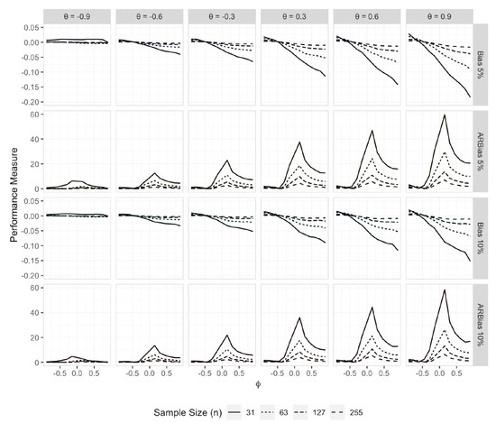
Figure 2. Empirical bias and ARB (%) of the $\mathrm{W}{L}_1$ estimator of ${\varphi }_1$ when the error distribution is a 5% or 10% contaminated bivariate normal distribution.

The extent of the bias is further emphasized by the ARB results, which show that for small sample sizes ($n=31$) and ${\varphi }_1$ near zero (in the range $-0.3$ to $+0.3$), the bias of ${\widehat{\varphi }}^{\mathrm{W}{L}_1}$ can range from 5% to 60% of the true value of ${\varphi }_1$ as $\theta$ varies from $-1$ to $+1$. For the smallest sample size ($n=31$), the relative bias remains considerably large for values of ${\varphi }_1$ greater than $-0.5$, provided $\theta$ does not approach $-1$. While the bias remains considerable in most cases for $n=63$ and $n=127$, it becomes negligible for larger sample sizes ($n=255$), except when ${\varphi }_1$ is near zero (in the range $-0.3$ to $+0.3$) and $\theta$ is positive.

4. Bias-Corrected WL₁ Estimators for the BAR(1) Model

In this section, we outline two bootstrap methods designed to correct the bias of the $\mathrm{W}{L}_1$ estimators, ${\widehat{\varphi }}_1^{\mathrm{W}{L}_1}$, for the autoregressive coefficient ${\varphi }_1$ in the BAR(1) model. Specifically, we introduce the single bootstrap bias-corrected version of ${\widehat{\varphi }}_1^{\mathrm{W}{L}_1}$, as well as a fast double bootstrap bias-corrected version.

The model-based bootstrap technique has been widely used to correct bias in the least squares (LS) estimation of the AR(1) model, with its properties thoroughly explored in the literature (see [25,26,27,28], among others). This approach involves generating a large number of bootstrap samples based on the estimated model parameters and resampled residuals. These samples are then used to compute multiple replicates of the estimator, which allows for the estimation of the sampling distribution, variance, and bias of the estimator. Recently, ref. [13] extended this method to correct bias in the LS estimation of the BAR(1) model coefficients. In this section, we focus on describing two model-based bootstrap bias correction methods specifically designed for the BAR(1) model.

We begin by rewriting the BAR(1) model, originally presented in Equation (1), as follows:

$$\begin{array}{cc}\hfill X_{2t}=& {\varphi }_0+{\varphi }_1{X}_t+{\epsilon }_{2t},\hfill \\ \hfill X_{2t+1}=& {\varphi }_0+{\varphi }_1{X}_t+{\epsilon }_{2t+1},\hfill \end{array}$$

for $t\ge 1$. Here, $X_{2t}$ and $X_{2t+1}$ represent the observations for the two daughter nodes branching from $X_t$.

The single bootstrap bias correction procedure for the autoregressive coefficient in the BAR(1) model is described in Algorithm 1. It is important to note that the bias in the corrected estimate, ${\widehat{\varphi }}_1^{\mathrm{SBC}}$, is of the order $O\left(n^{-2}\right)$, whereas the original estimator, ${\widehat{\varphi }}_1^{\mathrm{W}{L}_1}$, shows bias of the order $O\left(n^{-1}\right)$.

Algorithm 1 Single bootstrap bias-corrected $\mathrm{W}{L}_1$ estimation for ${\varphi }_1$ (SBC).

Input Observed tree: ${\mathbf{X}}^n=(X_1,X_2,\cdots ,X_n)$ $\mathrm{W}{L}_1$ estimates of the BAR(1) model coefficients: ${\widehat{\varphi }}_0^{\mathrm{W}{L}_1}$ and ${\widehat{\varphi }}_1^{\mathrm{W}{L}_1}$ Centered residuals: ${\tilde{\epsilon }}_t={\widehat{\epsilon }}_t-{(n-1)}^{-1}{\sum }_{i=2}^n{\widehat{\epsilon }}_i$ for $t\ge 2$ Number of bootstrap resamples: B  1: for each $b\leftarrow 1$ to B do  2:     Set $X_{1,b}^{\ast }=X^0$, the final observation from an initial binary tree of size $n^0=31$, where $X_1$ is the first observation in the original tree  3:     for each $j\leftarrow 1$ to $m=(n-1)/2$ do  4:         Sample with replacement a pair $({\tilde{\epsilon }}_{2j,b}^{\ast },{\tilde{\epsilon }}_{2j+1,b}^{\ast })$ from the set of pairs $\{({\tilde{\epsilon }}_{2t},{\tilde{\epsilon }}_{2t+1});t\ge 1\}$  5:         Compute $$X_{2j,b}^{\ast }={\widehat{\varphi }}_0^{\mathrm{W}{L}_1}+{\widehat{\varphi }}_1^{\mathrm{W}{L}_1}{X}_{j,b}^{\ast }+{\tilde{\epsilon }}_{2j,b}^{\ast },$$ $$X_{2j+1,b}^{\ast }={\widehat{\varphi }}_0^{\mathrm{W}{L}_1}+{\widehat{\varphi }}_1^{\mathrm{W}{L}_1}{X}_{j,b}^{\ast }+{\tilde{\epsilon }}_{2j+1,b}^{\ast }$$  6:     end for  7:     Construct the bootstrap tree ${\mathbf{X}}_b^{\ast n}=(X_{1,b}^{\ast },X_{2,b}^{\ast },\cdots ,X_{n,b}^{\ast })$  8:     Compute the $\mathrm{W}{L}_1$ estimate ${\widehat{\varphi }}_{1_b}^{\ast }$ from ${\mathbf{X}}_b^{\ast n}$  9: end for 10: Estimate the bias of ${\widehat{\varphi }}_1^{\mathrm{W}{L}_1}$ as ${\widehat{\beta }}_{{\widehat{\varphi }}_1^{\mathrm{W}{L}_1}}={\displaystyle \frac{1}{B}}{\displaystyle \sum _{b=1}^B}({\widehat{\varphi }}_{1_b}^{\ast }-{\widehat{\varphi }}_1^{\mathrm{W}{L}_1})$ Output: The single bootstrap bias-corrected $\mathrm{W}{L}_1$ estimate of ${\varphi }_1$ is given by $${\widehat{\varphi }}_1^{\mathrm{SBC}}={\widehat{\varphi }}_1^{\mathrm{W}{L}_1}-{\widehat{\beta }}_{{\widehat{\varphi }}_1^{\mathrm{W}{L}_1}}$$

The double bootstrap technique involves performing the single bootstrap procedure twice. This method has been shown to enhance the accuracy of bootstrap bias correction in the AR(1) model (e.g., [29,30,31,32]), and similarly for the BAR(1) model (see [13]). However, a notable drawback of the standard double bootstrap method is its high computational cost. To address this issue, a modified double bootstrap bias correction algorithm, referred to as the fast double bootstrap, was proposed by [33]. This algorithm offers greater computational efficiency compared to the traditional double bootstrap, as it requires only one bootstrap resample in phase 2 (i.e., $B_2=1$) for each bootstrap sample generated in phase 1, in contrast to the conventional double bootstrap, which generates $B_2$ resamples within each phase 1 bootstrap sample. Consequently, while the computational complexity of the standard double bootstrap algorithm is of the order $O\left(B_1{B}_2\right)$, the fast double bootstrap reduces this to $O\left(B_1\right)$. Despite this significant reduction in computational cost, ref. [13] observed that the bias correction performance of both algorithms remains comparable. The fast double bootstrap approach for correcting the bias in the $\mathrm{W}{L}_1$ estimator of ${\varphi }_1$ under the BAR(1) model is outlined in Algorithm 2.

Algorithm 2 Fast double bootstrap bias-corrected $\mathrm{W}{L}_1$ estimation for ${\varphi }_1$ (FDBC).

Input: Observed tree: ${\mathbf{X}}^n=(X_1,X_2,\dots ,X_n)$ $\mathrm{W}{L}_1$ estimates of the BAR(1) model coefficients: ${\widehat{\varphi }}_0^{\mathrm{W}{L}_1}$ and ${\widehat{\varphi }}_1^{\mathrm{W}{L}_1}$ Centered residuals: ${\tilde{\epsilon }}_t={\widehat{\epsilon }}_t-{(n-1)}^{-1}{\sum }_{i=2}^n{\widehat{\epsilon }}_i$, for $t\ge 2$ Number of phase 1 bootstrap resamples: $B_1$ Number of phase 2 bootstrap resamples: $B_2$  1: for each $b\leftarrow 1$ to $B_1$ do  2:     Set $X_{1,b}^{\ast }=X^0$, where $X^0$ is the last observation in an initial binary tree of size $n^0=31$, with $X_1$ as the first observation in ${\mathbf{X}}^n$  3:     for each $j\leftarrow 1$ to $m=(n-1)/2$ do  4:         Sample with replacement a pair $({\tilde{\epsilon }}_{2j,b}^{\ast },{\tilde{\epsilon }}_{2j+1,b}^{\ast })$ from the set $\{({\tilde{\epsilon }}_{2t},{\tilde{\epsilon }}_{2t+1})\mid t\ge 1\}$  5:         Compute $$X_{2j,b}^{\ast }={\widehat{\varphi }}_0^{\mathrm{W}{L}_1}+{\widehat{\varphi }}_1^{\mathrm{W}{L}_1}{X}_{j,b}^{\ast }+{\tilde{\epsilon }}_{2j,b}^{\ast },$$ $$X_{2j+1,b}^{\ast }={\widehat{\varphi }}_0^{\mathrm{W}{L}_1}+{\widehat{\varphi }}_1^{\mathrm{W}{L}_1}{X}_{j,b}^{\ast }+{\tilde{\epsilon }}_{2j+1,b}^{\ast }$$  6:     end for  7:     Construct the bootstrap tree ${\mathbf{X}}_b^{\ast n}=(X_{1,b}^{\ast },X_{2,b}^{\ast },\dots ,X_{n,b}^{\ast })$  8:     Compute the first-phase bootstrap $\mathrm{W}{L}_1$ estimates ${\widehat{\varphi }}_{0_b}^{\ast }$ and ${\widehat{\varphi }}_{1_b}^{\ast }$ from ${\mathbf{X}}_b^{\ast n}$  9:     Obtain the first-phase bootstrap residuals: $${\widehat{\epsilon }}_{2t,b}^{\ast }=X_{2t,b}^{\ast }-({\widehat{\varphi }}_{0_b}^{\ast }+{\widehat{\varphi }}_{1_b}^{\ast }{X}_{t,b}^{\ast }),$$ $${\widehat{\epsilon }}_{2t+1,b}^{\ast }=X_{2t+1,b}^{\ast }-({\widehat{\varphi }}_{0_b}^{\ast }+{\widehat{\varphi }}_{1_b}^{\ast }{X}_{t,b}^{\ast }),t\ge 1$$ 10:     Compute centered bootstrap residuals: $${\tilde{\tilde{\epsilon }}}_{t,b}^{\ast }={\widehat{\epsilon }}_{t,b}^{\ast }-{(n-1)}^{-1}\sum _{i=2}^n{\widehat{\epsilon }}_{i,b}^{\ast },t\ge 2$$ 11:     for each $k\leftarrow 1$ to $B_2=1$ do 12:         Apply steps 2–6 to ${\mathbf{X}}_b^{\ast n}$ using ${\widehat{\varphi }}_{0_b}^{\ast }$, ${\widehat{\varphi }}_{1_b}^{\ast }$, and the centered residuals ${\tilde{\tilde{\epsilon }}}_{t,b}^{\ast }$ 13:         Construct the second-phase bootstrap tree ${\mathbf{X}}_{k,b}^{\ast \ast n}=(X_{1,kb}^{\ast \ast },X_{2,kb}^{\ast \ast },\dots ,X_{n,kb}^{\ast \ast })$ 14:         Compute the second-phase bootstrap $\mathrm{W}{L}_1$ estimate ${\widehat{\varphi }}_{1_{kb}}^{\ast \ast }$ from ${\mathbf{X}}_{k,b}^{\ast \ast n}$ 15:     end for 16: end for 17: Estimate the single bootstrap bias of ${\widehat{\varphi }}_1^{\mathrm{W}{L}_1}$: $${\widehat{\beta }}_{{\widehat{\varphi }}_1^{\mathrm{W}{L}_1}}={\displaystyle \frac{1}{B_1}}\sum _{b=1}^{B_1}({\widehat{\varphi }}_{1_b}^{\ast }-{\widehat{\varphi }}_1^{\mathrm{W}{L}_1})$$ 18: Compute the double bootstrap bias adjustment factor: $${\widehat{\gamma }}_{{\widehat{\varphi }}_1^{\mathrm{W}{L}_1}}={\widehat{\beta }}_{{\widehat{\varphi }}_1^{\mathrm{W}{L}_1}}-{\displaystyle \frac{1}{B_1{B}_2}}\sum _{b=1}^{B_1}\sum _{k=1}^{B_2}({\widehat{\varphi }}_{1_{kb}}^{\ast \ast }-{\widehat{\varphi }}_{1_b}^{\ast })$$ Output: The fast double bootstrap bias-corrected $\mathrm{W}{L}_1$ estimate for ${\varphi }_1$: $${\widehat{\varphi }}_1^{\mathrm{FDBC}}={\widehat{\varphi }}_1^{\mathrm{W}{L}_1}-{\widehat{\beta }}_{{\widehat{\varphi }}_1^{\mathrm{W}{L}_1}}-{\widehat{\gamma }}_{{\widehat{\varphi }}_1^{\mathrm{W}{L}_1}}$$

In each bootstrap iteration, the initial tree is generated from a BAR(1) model with coefficients set to the observed $\mathrm{W}{L}_1$ estimates, ${\widehat{\varphi }}_0^{\mathrm{W}{L}_1}$ and ${\widehat{\varphi }}_1^{\mathrm{W}{L}_1}$, while the errors are sampled in pairs from the centered residuals. It is important to note that using $X_1$ from the observed tree as the initial observation in all bootstrap trees could introduce artificial correlation among the bootstrap samples. This issue may become more significant in higher-order BAR(p) models, where $2^p-1$ initial observations are required. In such cases, our method utilizes the final $2^p-1$ observations from the initial tree to avoid this potential problem. Any appropriate initial tree size, $n^0$, can be chosen. The suggested size of $n^0=31$ provides a reasonable compromise between computational efficiency and result stability.

5. Empirical Results

In this section, we present the findings of an empirical investigation aimed at (i) evaluating the effectiveness of the proposed bias correction methods for the $\mathrm{W}{L}_1$ estimator of the autoregressive coefficient in the BAR(1) model, and (ii) comparing the relative performance of these bias correction techniques. This study involved extensive simulations, with all computations conducted in R (version 4.1.3; [34]). The simulations were performed using the research computing resources of the Longleaf Cluster at the University of North Carolina at Chapel Hill, USA. This SLURM-managed cluster includes a machine equipped with an Intel Xeon E5-2699Av4 processor, featuring a 2.4 GHz clock speed, 44 cores, and 512 GB of memory, which enables efficient handling of large-scale computational demands. The simulations utilized 42 of the 44 available cores via the parallel package, while bifurcating trees were generated using the bifurcatingr package [35].

The “core” process follows the model described in (1), adhering to the same variance–covariance matrix. The “observed” process is defined as

$$X_t^{\ast }=X_t+V_t,t\ge 1.$$

(6)

In this definition, when $V_t=0$ for all t, the “observed” process aligns with the “core” process, and any deviations are attributed to the distribution of the errors. As noted by [36], these deviations are referred to as the innovation outliers (IOs). In this, the distribution of errors is typically characterized by heavy tails. On the other hand, when $V_t\ne 0$, the process corresponds to the additive outliers (AOs) [36]. In this case, $V_t$ follows a mixed distribution given by $(1-\gamma ){\delta }_0(·)+\gamma G(·)$, where $\gamma$ represents the contamination proportion, ${\delta }_0$ denotes a point mass at zero, and G is the contaminating distribution function. For our simulations, G was selected as a $N({\mu }_2,{\sigma }_c^2)$ distribution. Therefore, the distribution of $V_t$ can be expressed as

$$BCN(\gamma ,{\mu }_1,{\mathbf{\Sigma }}_{{\epsilon }_t},{\mu }_2,{\mathbf{\Sigma }}_{{\sigma }_c^2})=(1-\gamma )BN({\mu }_1,{\mathbf{\Sigma }}_{{\epsilon }_t})+\gamma BN({\mu }_2,{\mathbf{\Sigma }}_{{\sigma }_c^2}),$$

(7)

where $BCN(·)$ denotes a bivariate contaminated normal distribution with a specified mean vector and variance-covariance matrix.

The variable $V_t$ is generated as a sequence of independent and identically distributed random variables. In the AO model, outliers are introduced through the incorporation of external influences into the core process, resulting in outliers that arise from factors beyond the error distribution.

In the context of our study, an outlier introduced into the design is referred to as a leverage point. We differentiate between two types of leverage points: “good” and “bad”. As demonstrated by [19], a leverage point is classified as “good” if it results in a small residual despite being an outlier in the design space. In contrast, it is considered “bad” if it results in a large residual. According to [19], the IO model tends to produce “good” leverage points with a relatively minimal impact on estimates. In contrast, the AO model generates “bad” leverage points that can significantly affect estimates, even those that are robust [12].

5.1. Simulation Setup

The simulations contain a range of scenarios defined by varying sample sizes n, maternal correlation levels ${\varphi }_1$, and error correlations $\theta$, as outlined in Section 3. For each scenario, we generate $N=10,000$ trees and compute the $\mathrm{W}{L}_1$ estimator for the coefficient ${\varphi }_1$ from each tree. Specifically, we evaluate the $\mathrm{W}{L}_1$ estimator (${\widehat{\varphi }}^{\mathrm{W}{L}_1}$), the single bootstrap bias-corrected estimator (${\widehat{\varphi }}_1^{\mathrm{SBC}}$), and the fast double bootstrap bias-corrected estimator (${\widehat{\varphi }}_1^{\mathrm{FDBC}}$).

We excluded the case of $n=225$ from this simulation study, as the bias in ${\widehat{\varphi }}^{\mathrm{W}{L}_1}$ for this larger sample size was found to be negligible, as detailed in Section 3. This exclusion was implemented to facilitate computation time.

For both the ${\widehat{\varphi }}_1^{\mathrm{SBC}}$ and ${\widehat{\varphi }}_1^{\mathrm{FDBC}}$ estimators, the number of bootstrap replicates was set to $B=999$. The empirical bias and absolute relative bias (ARB) for each estimator were computed as outlined in Equations (4) and (5). Furthermore, the root mean squared error (RMSE) and mean absolute deviation (MAD) were calculated as follows:

$$\mathrm{RMSE}\left({\widehat{\varphi }}_1^{\mathrm{W}{L}_1}\right)=\sqrt{{\displaystyle \frac{1}{N}}{\displaystyle \sum _{j=1}^N}{({\widehat{\varphi }}_1^{\mathrm{W}{L}_1,\left(j\right)}-{\varphi }_1)}^2},$$

$$\mathrm{MAD}\left({\widehat{\varphi }}_1^{\mathrm{W}{L}_1}\right)={\displaystyle \frac{1}{N}}{\displaystyle \sum _{j=1}^N}\left|{\widehat{\varphi }}_1^{\mathrm{W}{L}_1,\left(j\right)}-{\varphi }_1\right|.$$

where ${\widehat{\varphi }}_1^{\mathrm{W}{L}_1,\left(j\right)}$ is the $\mathrm{W}{L}_1$ estimator from iteration $j=1,2,\cdots ,N$.

5.1.1. Innovation Outliers (IO) Model Setup

Under the innovation outlier (IO) model, where $V_t=0$, the “observed” process simplifies to the “core” process, as specified in Equation (1). The error distributions examined in this study include the bivariate standard normal distribution with correlation $\theta$, as well as four variants of the bivariate contaminated normal distributions. The contaminated distributions are characterized by different levels of contamination, specifically (1) contaminating variance of 25 with a contamination rate of 5%, (2) contaminating variance of 25 with a contamination rate of 10%, (3) contaminating variance of 49 with a contamination rate of 5%, and (4) contaminating variance of 49 with a contamination rate of 10%. These distributions are denoted as $\mathrm{BCN}(5\%,0,{\mathbf{\Sigma }}_1,0,{\mathbf{\Sigma }}_{25})$, $\mathrm{BCN}(10\%,0,{\mathbf{\Sigma }}_1,0,{\mathbf{\Sigma }}_{25})$, $\mathrm{BCN}(5\%,0,{\mathbf{\Sigma }}_1,0,{\mathbf{\Sigma }}_{49})$, $\mathrm{BCN}(10\%,0,{\mathbf{\Sigma }}_1,0,{\mathbf{\Sigma }}_{49})$, respectively. The chosen parameter settings for these bivariate contaminated normal distributions are intended to represent both “mild” and “extreme” contamination scenarios.

5.1.2. Additive Outliers (AO) Model Setup

Under the additive outlier (AO) model, the errors $\left({\epsilon }_{2t},{\epsilon }_{2t+1}\right)$ follow an innovation process modeled by a bivariate normal distribution with a zero mean, unit variance, and $\theta =0$. The distribution of $V_t$ is given by

$$V_t\sim (1-\gamma ){\delta }_0(·)+\gamma G(·),$$

where $\gamma$ represents the proportion of contamination, ${\delta }_0$ is a point mass at zero, and G is a contaminating distribution function. The “observed” process is defined as

$$X_t^{\ast }=X_t+V_t={\mathbf{Y}}_t^{\prime }\mathit{\varphi }+{\mathit{\epsilon }}_t+V_t,\mathrm{for}\mathrm{all}t\ge 1,$$

where ${\mathbf{Y}}_t^{\prime }\mathit{\varphi }$ represents the model component, ${\epsilon }_t$ is the error term, and $V_t$ represents the additive outlier.

The distributions considered for $V_t$ include the bivariate standard normal distribution with correlation $\theta$, as well as four bivariate contaminated normal distributions. These contaminated distributions have contaminating variances of 25 and 49, with contamination rates of 5% and 10%. Specifically, the distributions are (1) $\mathrm{BCN}(5\%,0,{\mathbf{\Sigma }}_1,0,{\mathbf{\Sigma }}_{25})$, (2) $\mathrm{BCN}(10\%,0,{\mathbf{\Sigma }}_1,0,{\mathbf{\Sigma }}_{25})$, (3) $\mathrm{BCN}(5\%,0,{\mathbf{\Sigma }}_1,0,{\mathbf{\Sigma }}_{49})$, and (4) $\mathrm{BCN}(10\%,0,{\mathbf{\Sigma }}_1,0,{\mathbf{\Sigma }}_{49})$. In addition, It is assumed that $V_t$ is independent of ${\epsilon }_t$.

5.2. Simulation Results

In this section, a summary of the simulation study’s results is presented in Figure 3, Figure 4, Figure 5, Figure 6, Figure 7, Figure 8, Figure 9 and Figure 10. Our analysis focuses on the absolute relative bias and root mean squared error (RMSE) for the $\mathrm{W}{L}_1$ estimator of ${\varphi }_1$, including both the single bootstrap and fast double bootstrap bias-corrected estimators. The key findings are outlined as follows:

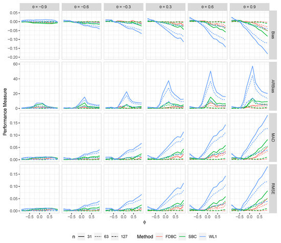
Figure 3. The bias, ARB, MAD, and RMSE of the $\mathrm{W}{L}_1$, single bootstrap bias-corrected $\mathrm{W}{L}_1$, and fast double bootstrap bias-corrected $\mathrm{W}{L}_1$ estimators as a function of ${\varphi }_1$ at different levels of $\theta$ under an IO model with a bivariate contaminated normal distribution, $BCN(5\%,0,{\mathbf{\Sigma }}_1,0,{\mathbf{\Sigma }}_{25})$.

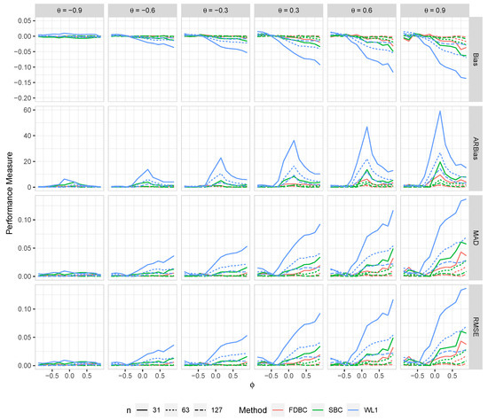
Figure 4. The bias, ARB, MAD, and RMSE of the $\mathrm{W}{L}_1$, single bootstrap bias-corrected $\mathrm{W}{L}_1$, and fast double bootstrap bias-corrected $\mathrm{W}{L}_1$ estimators as a function of ${\varphi }_1$ at different levels of $\theta$ under an IO model with a bivariate contaminated normal distribution, $BCN(10\%,0,{\mathbf{\Sigma }}_1,0,{\mathbf{\Sigma }}_{25})$.

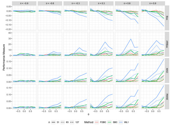
Figure 5. The bias, ARB, MAD, and RMSE of the $\mathrm{W}{L}_1$, single bootstrap bias-corrected $\mathrm{W}{L}_1$, and fast double bootstrap bias-corrected $\mathrm{W}{L}_1$ estimators as a function of ${\varphi }_1$ at different levels of $\theta$ under an IO model with a bivariate contaminated normal distribution, $BCN(5\%,0,{\mathbf{\Sigma }}_1,0,{\mathbf{\Sigma }}_{49})$.

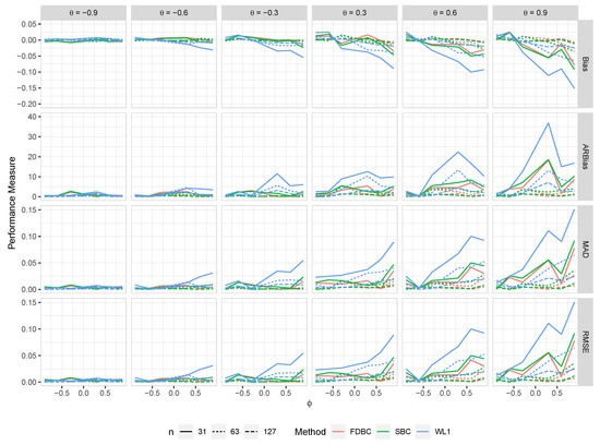
Figure 6. The bias, ARB, MAD, and RMSE of the $\mathrm{W}{L}_1$, single bootstrap bias-corrected $\mathrm{W}{L}_1$, and fast double bootstrap bias-corrected $\mathrm{W}{L}_1$ estimators as a function of ${\varphi }_1$ at different levels of $\theta$ under an IO model with a bivariate contaminated normal distribution, $BCN(10\%,0,{\mathbf{\Sigma }}_1,0,{\mathbf{\Sigma }}_{49})$.

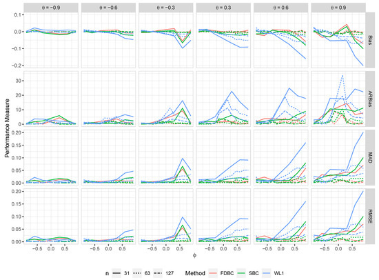
Figure 7. The bias, ARB, MAD, and RMSE of the $\mathrm{W}{L}_1$, single bootstrap bias-corrected $\mathrm{W}{L}_1$, and fast double bootstrap bias-corrected $\mathrm{W}{L}_1$ estimators as a function of ${\varphi }_1$ at different levels of $\theta$ under an AO model with a bivariate contaminated normal distribution, $BCN(5\%,0,{\mathbf{\Sigma }}_1,0,{\mathbf{\Sigma }}_{25})$.

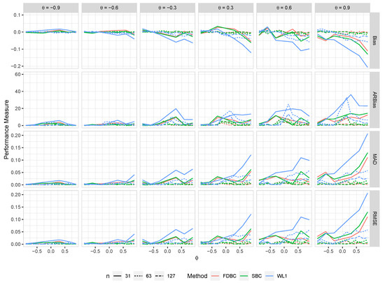
Figure 8. The bias, ARB, MAD, and RMSE of the $\mathrm{W}{L}_1$, single bootstrap bias-corrected $\mathrm{W}{L}_1$, and fast double bootstrap bias-corrected $\mathrm{W}{L}_1$ estimators as a function of ${\varphi }_1$ at different levels of $\theta$ under an AO model with a bivariate contaminated normal distribution, $BCN(10\%,0,{\mathbf{\Sigma }}_1,0,{\mathbf{\Sigma }}_{25})$.

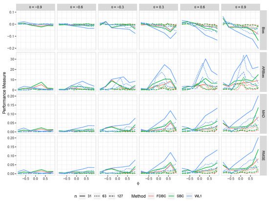
Figure 9. The bias, ARB, MAD, and RMSE of the $\mathrm{W}{L}_1$, single bootstrap bias-corrected $\mathrm{W}{L}_1$, and fast double bootstrap bias-corrected $\mathrm{W}{L}_1$ estimators as a function of ${\varphi }_1$ at different levels of $\theta$ under an AO model with a bivariate contaminated normal distribution, $BCN(5\%,0,{\mathbf{\Sigma }}_1,0,{\mathbf{\Sigma }}_{49})$.

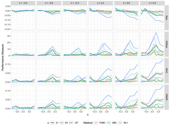
Figure 10. The bias, ARB, MAD, and RMSE of the $\mathrm{W}{L}_1$, single bootstrap bias-corrected $\mathrm{W}{L}_1$, and fast double bootstrap bias-corrected $\mathrm{W}{L}_1$ estimators as a function of ${\varphi }_1$ at different levels of $\theta$ under an AO model with a bivariate contaminated normal distribution, $BCN(10\%,0,{\mathbf{\Sigma }}_1,0,{\mathbf{\Sigma }}_{49})$.

• Generally, all proposed bias-correcting estimators substantially reduce the bias of the $\mathrm{W}{L}_1$ estimator across nearly all combinations of ${\varphi }_1$ and $\theta$, even with small sample sizes.
• Both the single bootstrap (${\widehat{\varphi }}_1^{\mathrm{SBC}}$) and fast double bootstrap (${\widehat{\varphi }}_1^{\mathrm{FDBC}}$) bias-corrected estimators effectively reduce bias. However, the fast double bootstrap estimator demonstrates superior performance compared to the single bootstrap estimator, particularly for small sample sizes (e.g., $n=31$). Despite this reduction, some residual bias persists when both $\theta$ and ${\varphi }_1$ are positive, with the bias increasing as $\theta$ and ${\varphi }_1$ approach the positive boundary.
• For larger sample sizes, $n=63$ and $n=127$, the fast double bootstrap estimator generally outperforms the single bootstrap estimator, though their performances are sometimes comparable. It is important to note that the fast double bootstrap method requires more computational time compared to the single bootstrap method.
• Both bootstrap methods lead to significant reductions in RMSE and mean absolute deviation (MAD) compared to the $\mathrm{W}{L}_1$ estimator across all sample sizes and positive values of $\theta$.
• The bias reduction achieved by both bootstrap estimators is particularly notable for ${\varphi }_1$ values near the boundaries (−1, +1), especially for small sample sizes (e.g., $n=31$). Additionally, the fast double bootstrap method outperforms the single bootstrap method in mitigating bias in the $\mathrm{W}{L}_1$ estimators.

Overall, these findings indicate that both the single and fast double bootstrap bias-corrected estimators are suitable for reducing bias in the $\mathrm{W}{L}_1$ estimation for the BAR(1) model under most combinations of ${\varphi }_1$ and $\theta$. Although the fast double bootstrap method is more effective in reducing bias, it requires more computational resources. Consequently, the single bootstrap approach may be preferred for its computational efficiency.

5.3. Application

In this study, we applied the artificial cell lineage data introduced by [12]. This dataset serves as an effective example to demonstrate the accuracy of the proposed bias correction methods. The dataset contains real cell lineage data originally sourced from [5], and it is visually represented in the tree diagram in Figure 1. This diagram includes 31 observations across four generations, representing the lifetimes of E. coli cells in minutes.

In this dataset, no natural outliers were present in the original E. coli lineage. However, ref. [12] introduced three artificial outliers at observations $X_1=60$, $X_5=60$, and $X_{11}=65$. Figure 11 illustrates the artificial outliers introduced to the original dataset. As a result, the lag-one scatter plot in Figure 12 identifies a total of seven outliers. Among these, the point (17, 60) is notable as an outlier in the response space, while the point (60, 65) is identified as an outlier in both the response and factor spaces. The remaining five points are identified as outliers in the factor space. Additionally, several points in the lower right-hand corner of the plot appear to be bad leverage points.

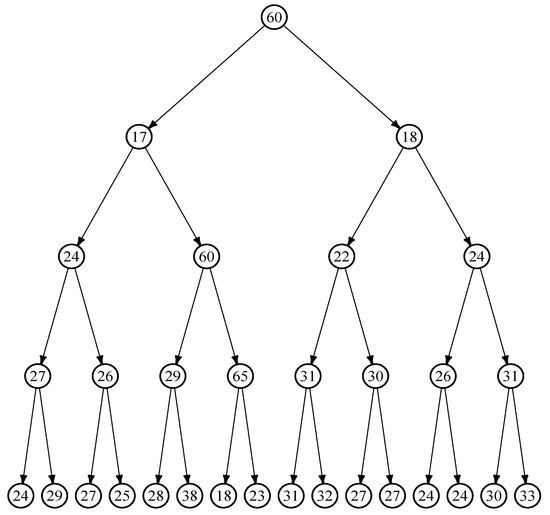
Figure 11. Artificial E. coli cell dataset, as presented in [12].

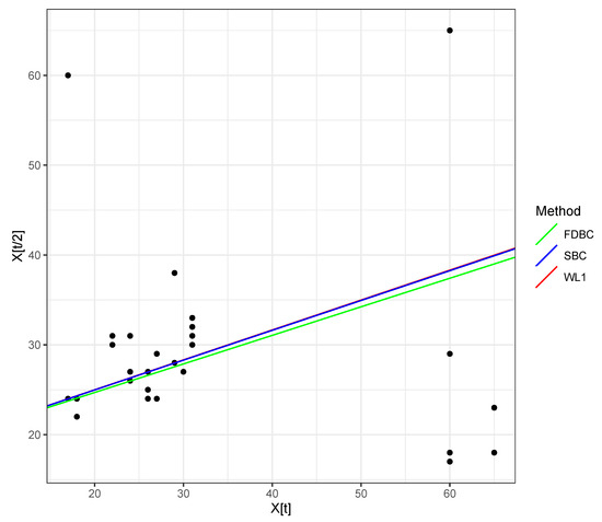
Figure 12. Lag(1) scatter plot for the artificial E. coli cell dataset, displaying the three autoregressive fitted lines corresponding to the weighted-$L_1$ (W$L_1$) estimates, as well as the single bootstrap (SBC) and fast double bootstrap (FDBC) bias correction methods for the estimated autoregressive coefficient ${\widehat{\varphi }}_1$ of the BAR(1) model.

The estimated W$L_1$ coefficients of the BAR(1) model for this dataset are ${\widehat{\varphi }}_0=18.333$ and ${\widehat{\varphi }}_1=0.333$. The bias-corrected estimates of ${\widehat{\varphi }}_1$ based on the single bootstrap and fast double bootstrap approaches are $0.332$ and $0.318$, respectively. The corresponding root mean squared error (RMSE) values for the W$L_1$ estimation, along with the bias-corrected estimates based on single and fast double bootstrap approaches, are $11.526$, $11.518$, and $11.417$, respectively. These RMSE results demonstrate the effectiveness of the bias correction methods in reducing bias in the W$L_1$ estimates for the coefficients of the BAR(1) model, leading to improved data fitting, particularly for a small sample size. Figure 12 displays the fitted autoregression lines for the W$L_1$ estimates, along with the bias correction methods based on the single and fast double bootstrap approaches.

6. Conclusions

In this study, we revisited the weighted $L_1$ (W$L_1$) estimator within the framework of first-order bifurcating autoregressive BAR(1) models. While the W$L_1$ estimator is known for its robustness to outliers, it can show substantial bias for small and moderate sample sizes, akin to the least squares estimator. The extent and direction of this bias are influenced by the autoregressive coefficient (${\varphi }_1$) and the correlation between model errors ($\theta$).

To address this issue, we introduced bias-corrected versions of the W$L_1$ estimator using the bootstrap method. Specifically, we developed the single bootstrap and fast double bootstrap bias-corrected W$L_1$ estimators. Our extensive empirical analysis demonstrated that these bootstrap bias-corrected estimators effectively reduce the bias inherent in the W$L_1$ estimator. The observed reduction in bias corresponded with a decreased root mean squared error (RMSE), thereby enhancing the overall efficiency of the corrected estimators. Although the fast double bootstrap method is somewhat more computationally demanding than the single bootstrap, it consistently outperformed the latter in most of the scenarios considered in our simulations.

While our research primarily focused on BAR(1) models, future investigations will extend to higher-order BAR models (i.e., BAR($p>1$)). Additionally, we plan to explore how bias and its correction impact related inferences, such as confidence intervals and hypothesis tests, to further assess the practical implications of our findings.

References

- Cowan, R. Statistical Concepts in the Analysis of Cell Lineage Data. In Proceedings of the 1983 Workshop Cell Growth Division; Latrobe University: Melbourne, Australia, 1984; pp. 18–22. [Google Scholar]
- Hawkins, E.D.; Markham, J.F.; McGuinness, L.P.; Hodgkin, P.D. A single-cell pedigree analysis of alternative stochastic lymphocyte fates. Proc. Natl. Acad. Sci. USA 2009, 106, 13457–13462. [Google Scholar] [CrossRef] [PubMed]
- Kimmel, M.; Axelrod, D. Branching Processes in Biology; Springer: New York, NY, USA, 2005. [Google Scholar]
- Sandler, O.; Mizrahi, S.P.; Weiss, N.; Agam, O.; Simon, I.; Balaban, N.Q. Lineage correlations of single cell division time as a probe of cell-cycle dynamics. Nature 2015, 519, 468–471. [Google Scholar] [CrossRef] [PubMed]
- Cowan, R.; Staudte, R. The Bifurcating Autoregression Model in Cell Lineage Studies. Biometrics 1986, 42, 769–783. [Google Scholar] [CrossRef] [PubMed]
- Huggins, R.M. A law of large numbers for the bifurcating autoregressive process. Commun. Statistics. Stoch. Model. 1995, 11, 273–278. [Google Scholar] [CrossRef]
- Bui, Q.; Huggins, R. Inference for the random coefficients bifurcating autoregressive model for cell lineage studies. J. Stat. Plan. Inference 1999, 81, 253–262. [Google Scholar] [CrossRef]
- Huggins, R.M.; Basawa, I.V. Extensions of the Bifurcating Autoregressive Model for Cell Lineage Studies. J. Appl. Probab. 1999, 36, 1225–1233. [Google Scholar] [CrossRef]
- Huggins, R.; Basawa, I. Inference for the extended bifurcating autoregressive model for cell lineage studies. Aust. New Zealand J. Stat. 2000, 42, 423–432. [Google Scholar] [CrossRef]
- Zhou, J.; Basawa, I. Least-squares estimation for bifurcating autoregressive processes. Stat. Probab. Lett. 2005, 74, 77–88. [Google Scholar] [CrossRef]
- Terpstra, J.T.; Elbayoumi, T. A law of large numbers result for a bifurcating process with an infinite moving average representation. Stat. Probab. Lett. 2012, 82, 123–129. [Google Scholar] [CrossRef]
- Elbayoumi, T.; Terpstra, J. Weighted L1-Estimates for the First-order Bifurcating Autoregressive Model. Commun. Stat.-Simul. Comput. 2016, 45, 2991–3013. [Google Scholar] [CrossRef]
- Elbayoumi, T.M.; Mostafa, S.A. On the estimation bias in first-order bifurcating autoregressive models. Stat 2021, 10, e342. [Google Scholar] [CrossRef]
- Hurwicz, L. Least squares bias in time series. Stat. Inference Dyn. Econ. Model. 1950, 10, 365–383. [Google Scholar]
- Huggins, R.M.; Marschner, I.C. Robust Analysis of the Bifurcating Autoregressive Model in Cell Lineage Studies. Aust. New Zealand J. Stat. 1991, 33, 209–220. [Google Scholar] [CrossRef]
- Staudte, R.G. A bifurcating autoregression model for cell lineages with variable generation means. J. Theor. Biol. 1992, 156, 183–195. [Google Scholar] [CrossRef]
- MacKinnon, J.G.; Smith, A.A. Approximate bias correction in econometrics. J. Econom. 1998, 85, 205–230. [Google Scholar] [CrossRef]
- Reber, J.C.; Terpstra, J.T.; Chen, X. Weighted L1-estimates for a VAR(p) time series model. J. Nonparametr. Stat. 2008, 20, 395–411. [Google Scholar] [CrossRef]
- Rousseeuw, P.J.; Leroy, A.M. Robust Regression and Outlier Detection; John Wiley and Sons: New York, NY, USA, 1987. [Google Scholar]
- Naranjo, J.D.; Hettmansperger, T.P. Bounded Influence Rank Regression. J. R. Stat. Soc. Ser. (Methodological) 1994, 56, 209–220. [Google Scholar] [CrossRef]
- Chang, W.H.; McKean, J.W.; Naranjo, J.D.; Sheather, S.J. High-Breakdown Rank Regression. J. Am. Stat. Assoc. 1999, 94, 205–219. [Google Scholar] [CrossRef]
- Terpstra, J.T.; McKean, J.W.; Naranjo, J.D. Highly efficient weighted for autoregression Wilcoxon estimates for autoregression. Statistics 2000, 35, 45–80. [Google Scholar] [CrossRef]
- McKean, J.M.; Schrader, R.M. A comparison of methods for studentizing the sample median. Commun. Stat. Part B-Simul. Comput. 1984, 6, 751–773. [Google Scholar] [CrossRef]
- Sheather, S.J. Assessing the accuracy of the sample median: Estimated standard errors versus interpolated confidence interval. In Statistical Data Analysis Based on the L1-Norm and Related Methods; Dodge, Y., Ed.; Birkhäuser: Basel, Switzerland, 1987; Volume 6, pp. 203–216. [Google Scholar]
- Berkowitz, J.; Kilian, L. Recent developments in bootstrapping time series. Econom. Rev. 2000, 19, 1–48. [Google Scholar] [CrossRef]
- Tanizaki, H.; Hamori, S.; Matsubayashi, Y. On least-squares bias in the AR(p) models: Bias correction using the bootstrap methods. Stat. Pap. 2006, 47, 109–124. [Google Scholar] [CrossRef]
- Patterson, K. Bias Reduction through First-order Mean Correction, Bootstrapping and Recursive Mean Adjustment. J. Appl. Stat. 2007, 34, 23–45. [Google Scholar] [CrossRef]
- Liu-Evans, G.D.; Phillips, G.D. Bootstrap, Jackknife and COLS: Bias and Mean Squared Error in Estimation of Autoregressive Models. J. Time Ser. Econom. 2012, 4, 1–33. [Google Scholar] [CrossRef]
- Hall, P. The Bootstrap and Edgeworth Expansion; Springer: New York, NY, USA, 1992. [Google Scholar]
- Lee, S.M.S.; Young, G.A. The effect of Monte Carlo approximation on coverage error of double-bootstrap confidence intervals. J. R. Stat. Soc. Ser. B Stat. Methodol. 1999, 61, 353–366. [Google Scholar] [CrossRef]
- Shi, S.G. Accurate and Efficient Double-bootstrap Confidence Limit Method. Comput. Stat. Data Anal. 1992, 13, 21–32. [Google Scholar] [CrossRef]
- Chang, J.; Hall, P. Double-bootstrap methods that use a single double-bootstrap simulation. Biometrika 2015, 102, 203–214. [Google Scholar] [CrossRef]
- Ouysse, R. A Fast Iterated Bootstrap Procedure for Approximating the Small-Sample Bias. Commun. Stat.—Simul. Comput. 2013, 42, 1472–1494. [Google Scholar] [CrossRef]
- R Core Team. R: A Language and Environment for Statistical Computing; R Foundation for Statistical Computing: Vienna, Austria, 2022. [Google Scholar]
- Elbayoumi, T.; Mostafa, S. Bifurcatingr: Bifurcating Autoregressive Models, R package version 2.1.0, 2024. Available online: https://CRAN.R-project.org/package=bifurcatingr (accessed on 8 April 2024).
- Fox, A.J. Outliers in Time Series. J. R. Stat. Soc. B 1972, 34, 350–363. [Google Scholar] [CrossRef]
Disclaimer/Publisher’s Note: The statements, opinions and data contained in all publications are solely those of the individual author(s) and contributor(s) and not of MDPI and/or the editor(s). MDPI and/or the editor(s) disclaim responsibility for any injury to people or property resulting from any ideas, methods, instructions or products referred to in the content. |
© 2024 by the authors. Licensee MDPI, Basel, Switzerland. This article is an open access article distributed under the terms and conditions of the Creative Commons Attribution (CC BY) license (https://creativecommons.org/licenses/by/4.0/).