reflimLOD: A Modified reflimR Approach for Estimating Reference Limits with Tolerance for Values Below the Lower Limit of Detection (LOD)

Abstract

Reference intervals are indispensable for the interpretation of medical laboratory results to distinguish “normal” from “pathological” values. Recently, indirect methods have been published, which estimate reference intervals from a mixture of normal and pathological values based on certain statistical assumptions on the distribution of the values from the healthy population. Some analytes face the problem that a significant proportion of the measurements are below the limit of detection ($\mathrm{LOD}$), meaning that there are no quantitative data for these values, only the information that they are smaller than the $\mathrm{LOD}$. Standard statistical methods for reference interval estimation are not designed to incorporate values below the $\mathrm{LOD}$. We propose two variants of the indirect method reflimR—a quantile- and maximum likelihood-based estimator—that are able to cope with values below the $\mathrm{LOD}$. We show, based on theoretical analyses, simulation experiments, and real data, that our approach yields good estimates for the reference interval, even when the values below the $\mathrm{LOD}$ contribute a substantial proportion to the data.

1. Introduction

Reference intervals (RIs) are crucial for interpreting laboratory results in clinical practice. Defined as the central 95% range of a presumably healthy population’s values, RIs help determine whether a lab result should be considered “pathological” or not. Traditionally, these intervals are established using direct methods, which involve measuring analyte levels in a sufficiently large and well-characterized healthy reference group [1]. The 2.5 and 97.5 percentiles, called the lower and upper reference limit, are then determined either directly from data or from a distribution model, assuming a normal distribution for example [2,3,4]. While other ranges (such as the central 90% or 99%) could theoretically serve as a reference, the guideline [2] has specifically defined the central 95% as the standard. Hence, this 95% range is mandatory for laboratory use.

Due to economic, organizational, and ethical challenges with the recruitment of reference individuals, it has become common practice to estimate reference intervals using so-called indirect methods [2,4]. Unlike direct methods, they utilize routine laboratory data, which can easily be retrieved from laboratory information systems. This approach inherently includes both normal and pathological results, necessitating advanced statistical techniques to isolate the healthy subset from the mixed population for accurate RI estimation [2,4,5]. Two R packages for the implementation of the indirect approach in laboratory medicine are publicly available on CRAN: reflimR [3] and refineR [6].

Both direct and indirect approaches are effective provided that the 2.5 percentile is above the lower limit of detection ($\mathrm{LOD}$) of the analytical method. In most cases, this requirement is met. However, there are analytes, such as the cardiac marker troponin, for which the analytical sensitivity of the detection method is not sufficient to quantitatively measure concentrations around or even above the lower reference limit [7]. Therefore, low values are often reported as “below LOD” rather than a specific value. In the case of troponin T, low values are expressed as <3 μg/L for example.

In this paper, we propose a statistical method to address this problem. It is based on the assumption that the distribution of such measurements can be modeled with a truncated normal distribution after applying a Box–Cox transformation with an appropriate parameter $\lambda$ [2,4]. We explain the theoretical background of our approach and demonstrate its feasibility with simulated data. As practical examples, we demonstrate the accuracy of the method with real data.

Section 2 provides a formal definition of the problem of estimating reference intervals with values below the $\mathrm{LOD}$. A short review of indirect methods for reference interval estimation and their suitability to handle values below the $\mathrm{LOD}$ is provided in Section 3. The new algorithm is derived and described in Section 4. Theoretical and simulation-based analyses as well as a validation with real data of our method are described in Section 5. The paper concludes by addressing the importance of reference interval estimation with values below $\mathrm{LOD}$ and discussing the assumptions and limitations of our approach.

2. Problem Formulation

The problem we consider here can be formulated as follows. We want to estimate the reference interval, i.e., the 2.5 and the 97.5 percentiles for a specific analyte within a healthy population. The sample used for the estimation originates from a mixed population with an unknown proportion of pathological values. This is the typical challenge faced by indirect methods when determining reference intervals. An additional issue is the problem that values below the $\mathrm{LOD}$ cannot be measured, so that our sample contains actual measurements coming from healthy and non-healthy individuals and a number of missing values. These missing values are not missing completely at random. We know that these are values below a known specified limit of detection $\mathrm{LOD}>0$.

Because of the contamination of our sample with pathological values, it is impossible to estimate the reference interval without additional assumptions. We impose the following three assumptions.

(i)

Values from the healthy population follow a (truncated) normal distribution $X\sim N\left(\mu ,{\sigma }^2,{\displaystyle \frac{-\frac{1}{\lambda }-\mu }{\sigma }},\infty \right)$, i.e., X is a random variable following a normal distribution truncated at ${\displaystyle \frac{-\frac{1}{\lambda }-\mu }{\sigma }}$ with expected value $\mu$ and variance ${\sigma }^2$ after a suitable Box–Cox transformation

$$t_{\lambda }\left(x\right)=\left\{\begin{array}{cc}{\displaystyle \frac{x^{\lambda }-1}{\lambda }}\hfill & \mathrm{if}\lambda \ne 0,\hfill \\ log\left(x\right)\hfill & \mathrm{if}\lambda =0.\hfill \end{array}\right.$$

(1)

with parameter $\lambda \in [0,1]$. For $0<\lambda <1$, the truncation is necessary because the Box–Cox transformation can only be applied to positive values. We assume that the truncation has a negligible effect, i.e., $\mathsf{\Phi }\left({\displaystyle \frac{-\frac{1}{\lambda }-\mu }{\sigma }}\right)\approx 0$, where $\mathsf{\Phi }$ is the cumulative distribution function of the standard normal distribution. A Yeo–Johnson transformation [8] instead of the Box–Cox transformation could avoid the artificial truncation. However, it is common practice in laboratory medicine to stay with the Box–Cox transformation as analyte concentrations cannot be negative.

(ii)

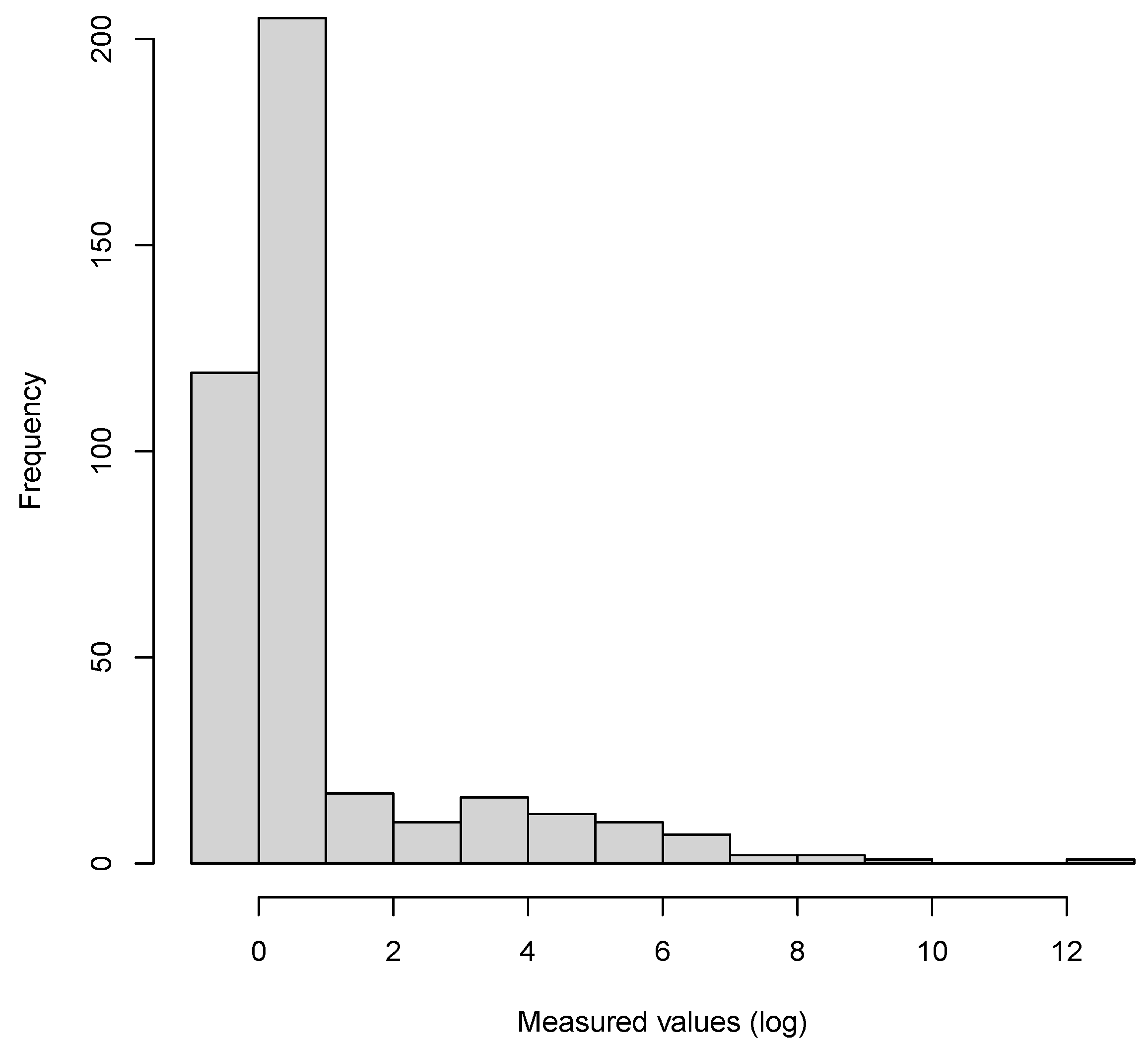
There is a limit of detection $\mathrm{LOD}>0$, i.e., for values below the $\mathrm{LOD}$, we cannot measure their exact value. We only have the information that the corresponding values are smaller than the LOD. We assume that less than 50% of the values from the healthy population are below the $\mathrm{LOD}$.

(iii)

Apart from the values from the healthy population, there can be additional pathological values. We make no specific assumption on the distribution of the pathological values except that they tend to be higher than the values from the healthy population and that no values from diseased individuals are below the $\mathrm{LOD}$ (see Section 6.2). We also assume that there are fewer pathological values than from the healthy population.

Assumption (i) is a standard assumption in more or less all indirect methods for reference interval estimation [3,6,9,10]. Assumption (ii) on the presence of values below the $\mathrm{LOD}$ is specific for our method. Assumption (iii) is usually formulated more generally in the sense that there can be pathologically high as well as pathologically low values. In our specific setting, it is impossible to identify pathologically low values because they would be below the $\mathrm{LOD}$ and nothing can be observed about their distribution. Therefore, we assume that only elevated pathological values occur. Whether this assumption is realistic will be discussed in Section 6.2.

Let $Y\sim N(\mu ,{\sigma }^2,{\displaystyle \frac{-\frac{1}{\lambda }-\mu }{\sigma }},\infty )$, i.e., Y is a random variable following a normal distribution with expected value $\mu$ and variance ${\sigma }^2$, which is left-truncated at ${\displaystyle \frac{-\frac{1}{\lambda }-\mu }{\sigma }}$. We observe the random variable $t_{\lambda }^{-1}\left(Y\right)$, where $t_{\lambda }^{-1}$ is the inverse Box–Cox transformation

$$t_{\lambda }^{-1}\left(y\right)=\left\{\begin{array}{cc}{(\lambda y+1)}^{{\displaystyle \frac{1}{\lambda }}}\hfill & \mathrm{if}\lambda \ne 0,\hfill \\ e^y\hfill & \mathrm{if}\lambda =0.\hfill \end{array}\right.$$

(2)

Values for which $x=t_{\lambda }^{-1}\left(y\right)<\mathrm{LOD}$ holds will be observed as missing values. A sample of size n then consists of measurements $x_1,\dots ,x_{n-n_{\mathrm{LOD}}}\in \mathbb{R}$ from the distribution $t_{\lambda }^{-1}\left(Y_{\mathrm{LOD}}\right)$ where $Y_{\mathrm{LOD}}\sim N(\mu ,{\sigma }^2,t_{\lambda }\left(\mathrm{LOD}\right),\infty )$, and the number $n_{\mathrm{LOD}}\in \mathbb{N}$ of values below the $\mathrm{LOD}$.

For the reference interval, we need to estimate the 2.5 and the 97.5 percentile of the distribution $t_{\lambda }^{-1}\left(Y\right)$, which can also be derived from estimations of the parameters $\mu$ and $\sigma$. The $\mathrm{LOD}$ is a known parameter. The parameter $\lambda$ is either assumed to be known or is part of the estimation.

3. Related Work

A recommendation of the International Federation of Clinical Chemistry and Laboratory Medicine (IFCC) published in 2018 [2] offers an overview on indirect methods for reference interval estimation. However, since then, a variety of new methods have been proposed, some of which can at least theoretically offer solutions to the problem. The truncated minimum chi-square (TMC) approach [9] essentially uses a chi-squared test to find a subset of the Box–Cox transformed data that fits to a normal distribution. The estimation of the parameter $\lambda$ of the Box–Cox transformation is also part of the algorithm. Although this algorithm was not originally designed to handle values below the $\mathrm{LOD}$, a modified version [7] adjusts the binning of the ${\chi }^2$-test so that all values below the $\mathrm{LOD}$ are grouped into the lowest bin, making their actual values irrelevant. Unfortunately, the implementation of the algorithm is not publicly available.

The refineR approach [6] is another binning-based approach using the averaged shifted histogram method [11] to identify both the parameter $\lambda$ of the Box–Cox transformation and the normal sub-population among the Box–Cox-transformed values. Although it might be possible to adapt the refineR approach to data with values below the LOD, it cannot be performed in a straightforward manner as in the case of TMC approach due to use of the averaged shifted histogram method.

Concordet et al. [10] proposed an algorithm based on Gaussian mixture models by extending the usual expectation maximization (EM) approach by individual parameters $\lambda$ for the healthy and pathological population. This extended EM approach assumes that the values can be modelled by two inverse Box–Cox-transformed (truncated) normal distributions, i.e., this modified Gaussian mixture model uses only two clusters. Apart from this restrictive assumption, the authors did incorporate values below the $\mathrm{LOD}$ into their Gaussian mixture model.

The recently published R package reflimR [3] separates the estimation of the parameter $\lambda$ from the identification of the healthy population. Because the estimation of $\lambda$ involves high uncertainty and a wrong estimate of $\lambda$ affects the estimation of the reference interval only marginally unless a true $\lambda \approx 0$ is wrongly estimated by a value $\widehat{\lambda }\approx 1$ [12], reflimR distinguishes only between either a log-normal distribution ($\lambda =0$) or a normal distribution $\lambda =1$.

The reflimR method uses Bowley’s quartile skewness [13] for the decision of whether to assume a normal or a log-normal distribution for the values from the healthy population. This skewness measure is based on the sample quartiles and is therefore not suitable for a direct application to data with values below the $\mathrm{LOD}$. This is especially true when more than 25% of the values lie below the $\mathrm{LOD}$ because then the first quartile cannot be computed directly from the data.

After the decision has been made to log-transform or to leave the data as it is, reflimR uses an iterated truncation algorithm to estimate the range of the central 95% of the healthy population. The truncation algorithm computes the minimum $d_{\min }$ of the absolute differences of the median to the first and third quartile to truncate the data at the estimated 2.5 and 97.5 percentiles of the healthy population based on the assumption that their values follow a normal distribution after a possible logarithmic transformation. The truncation is carried out at the median $\pm c·d_{\min }$. The factor c can be derived from the normal distribution assumption and is therefore

$$c={\displaystyle \frac{{\mathsf{\Phi }}^{-1}\left(0.025\right)}{{\mathsf{\Phi }}^{-1}\left(0.25\right)}}\approx 2.905847$$

(3)

in the first step when no truncation has taken place. In all subsequent steps, when the data have already been truncated, the respective factor is

$$c={\displaystyle \frac{{\mathsf{\Phi }}^{-1}\left(0.025\right)}{{\mathsf{\Phi }}^{-1}\left(0.25·0.95+0.025\right)}}\approx 3.083367.$$

(4)

After convergence of the iterated truncation procedure, the reference interval can either be directly estimated by the truncation limits or based on estimates of the mean and standard deviation of the truncated normal distribution. Of course, if the data were log-transformed, the estimated reference interval must be back-transformed by an exponential function.

Because the truncation algorithm of reflimR is based on the sample quartiles, the same restrictions as for Bowley’s quartile skewness apply to data with values below the $\mathrm{LOD}$ if more than 25% of the values lie below $\mathrm{LOD}$.

The following section introduces modifications of the reflimR approach in order to handle values below $\mathrm{LOD}$.

4. A Modified Version of reflimR-Tolerating Values Below LOD

The modified version LODreflimR of reflimR differs in the following aspects from the standard version of reflimR.

(a)

In [14], it was suggested that the log-normal distribution should be the default assumption for the healthy population. LODreflimR either follows this recommendation and log-transforms the data or it provides estimated reference intervals for different values of the parameter $\lambda$ for the Box–Cox transformation and uses modified quantile–quantile plots to decide which value of $\lambda$ should be chosen. Details on the choice of $\lambda$ will be provided in Section 4.4.

(b)

The truncation algorithm is modified. The truncation of the standard version of reflimR is based on the differences of the median to the first and third quartiles, i.e., the smaller difference is used to iteratively estimate the 2.5 and 97.5 percentiles of the healthy population. The LOD version uses only the difference between the third quartile and the median to iteratively estimate the 97.5 percentile of the healthy population. When there are more than 25% of the values below the LOD, the first quartile cannot be computed anyway. In contrast to the standard version of reflimR, only values beyond the estimated 97.5 percentile are discarded, i.e., all small values including those below the $\mathrm{LOD}$ are kept. The underlying assumption is that there are no pathological small values. The modified truncation algorithm is described in Section 4.1.

(c)

The output of the standard version of reflimR directly provides estimates for the 2.5 and 97.5 percentiles of the healthy population by the truncation limits. The $\mathrm{LOD}$ version only provides an estimate for the upper truncation limit, i.e., an estimate for the 97.5 percentile but not for the 2.5 percentile. In Section 4.2, a very simple approach based on the $\mathrm{LOD}$ together with the upper truncation limit is introduced to obtain an estimate for the reference interval. Section 4.3 describes as an alternative: a maximum likelihood approach using all values between the $\mathrm{LOD}$ and the upper truncation limit.

4.1. Modified Truncation Algorithm

The modified truncation algorithm modTrunc assumes that the measured values and the $\mathrm{LOD}$ have already been transformed, such that the (transformed) values from the healthy population follow a normal distribution. When referring to the measured values and the $\mathrm{LOD}$ in this subsection, we specifically mean the already Box–Cox transformed values. The basis for modTrunc is the estimates of the median and the 75 percentile of the healthy population. The input for the algorithm consists of the (transformed) measured values x above the $\mathrm{LOD}$, the number $n_{\mathrm{LOD}}$ of values below the $\mathrm{LOD}$ and the (transformed) $\mathrm{LOD}$. As long as there are less than 50% of the values below the $\mathrm{LOD}$, we can easily estimate the median and the 75 percentile by simply extending the list of measured values x by $n_{\mathrm{LOD}}$ values below the $\mathrm{LOD}$, e.g., by appending $n_{\mathrm{LOD}}$ times the value $(\mathrm{LOD}-1)$ to x.

Assuming a normal distribution, we can estimate the 97.5 percentile t based on the sample median m and the sample 75 percentile $q_{75}$ by

$$t=m+(q_{75}-m)\ast {\displaystyle \frac{{\mathsf{\Phi }}^{-1}\left(0.975\right)}{{\mathsf{\Phi }}^{-1}\left(0.75\right)}}.$$

(5)

We then truncate the values at t. Because the measured values can include increased pathological values, the sample median and the sample 75 percentile $q_{75}$ tend to have a bias overestimating the median and the 75 percentile of the healthy population. Therefore, we iterate this truncation procedure. However, continuing to use Equation (5) after the first truncation step would introduce another bias, especially when there are no pathological values; or when all pathological values are already removed by the truncation, because we must then assume that we are dealing with values from a normal distribution truncated at the 97.5 percentile. The sample median and the sample 75 percentile of the truncated data would underestimate both quantiles. The median of the healthy population should therefore not be estimated by the sample median of the truncated data, but by the $100·p_{50}$ percentile where

$$p_{50}={\displaystyle \frac{0.5}{0.975}}.$$

(6)

The following considerations show why $p_{50}$ should be used. Consider the random variable $X_t$ resulting from the random variable X truncated at the upper value $t\in \mathbb{R}$. The cumulative distribution function of $X_t$ is then

$$F_{X_t}\left(x\right)=P(X_t\le x)=\left\{\begin{array}{cc}{\displaystyle \frac{P(X\le x)}{P(X\le t)}}\hfill & \mathrm{if}x\le t\hfill \\ 1,\hfill & \mathrm{otherwise}.\hfill \end{array}\right.$$

(7)

Let $\alpha \in (0,1)$. Then,

$$\alpha =P(X_t\le x)={\displaystyle \frac{P(X\le x)}{P(X\le t)}}$$

(8)

implies

$$\alpha ·P(X_t\le t)=P(X\le x).$$

(9)

This means that the $\alpha ·P(X\le t)$ quantile of X corresponds to the $\alpha$ quantile of $X_t$. Therefore, in order to estimate the $\beta$ quantile of X based on a sample from $X_t$, i.e.,

$$\beta =P(X\le x)=\alpha ·P(X\le t).$$

(10)

one could estimate the ${\displaystyle \frac{\beta }{P\left(X_t\right)}}$ of $X_t$. In our setting, the truncation is aimed at the 0.975 quantile, meaning that $P(X\le t)=0.975$ holds.

The same consideration applies to the estimation of the 75 percentile of the healthy population. Here, one should use the $100·p_{75}$ percentile of the truncated data, where

$$p_{75}={\displaystyle \frac{0.75}{0.975}}.$$

(11)

Algorithm 1 describes the iterative truncation procedure. For simplicity, we have not accounted for the termination without result in cases where at any iteration step the values below the $\mathrm{LOD}$ become the majority, making the estimation of the median impossible.

Algorithm 1 The modified truncation algorithm.
1:	procedure modTrunc(x,$n_{\mathrm{LOD}}$,$\mathrm{LOD}$)	▹ Input x: measured values
2:		▹$n_{\mathrm{LOD}}$: No. of values $<\mathrm{LOD}$
3:		▹$\mathrm{LOD}$: Level of detection
4:	$y\leftarrow (x,\underset{n_{\mathrm{LOD}}\mathrm{times}}{\underbrace{\mathrm{LOD}-1,\dots ,\mathrm{LOD}-1}})$	▹ The value $(\mathrm{LOD}-1)$ is appended
5:		▹$n_{\mathrm{LOD}}$ times to x
6:	$m\leftarrow$ median(y)	▹ Median of the measured values including $\mathrm{LOD}$s
7:	$q_{75}\leftarrow$ quantile(y,0.75)	▹ 75 percentile of the measured values
8:		▹ Including $\mathrm{LOD}$s
9:	$t\leftarrow m+(q_{75}-m)\ast {\displaystyle \frac{{\mathsf{\Phi }}^{-1}\left(0.975\right)}{{\mathsf{\Phi }}^{-1}\left(0.75\right)}}$	▹ Value for the upper truncation
10:	$y_{\mathrm{new}}\leftarrow \mathrm{truncate}(y,-\infty ,t)$	▹ Remove all values $>t$ from y.
11:	$p_{50}\leftarrow {\displaystyle \frac{0.5}{{\mathsf{\Phi }}^{-1}\left(0.975\right)}}$	▹ Equation (11)
12:	$p_{75}\leftarrow {\displaystyle \frac{0.75}{{\mathsf{\Phi }}^{-1}\left(0.975\right)}}$	▹ Equation (6)
13:	while $y_{\mathrm{new}}\ne y$ do	▹ Continue until no more values are truncated.
14:	$y\leftarrow y_{\mathrm{new}}$
15:	$m\leftarrow$ quantile($y,p_{50}$)
16:	$q_{75}\leftarrow$ quantile($y,p_{75}$)
17:	$t\leftarrow m+(q_{75}-m)\ast {\displaystyle \frac{{\mathsf{\Phi }}^{-1}\left(0.975\right)}{{\mathsf{\Phi }}^{-1}\left(0.75\right)}}$
18:	$y_{\mathrm{new}}\leftarrow \mathrm{truncate}(y,-\infty ,t)$	▹ Remove all values $>t$ from y.
19:	end while
20:	$y\leftarrow \mathrm{truncate}(y,\mathrm{LOD}-0.5,t)$	▹ Remove the artificial values below $\mathrm{LOD}$.
21:	return $y,t$	▹ The non-truncated values and the upper truncation limit
22:	end procedure

4.2. Quantile-Based Estimator: reflimLOD.Quant

After the termination of the modified truncation algorithm, the following pieces of information and data are available:

• An estimate of the 97.5 percentile ${\widehat{x}}_{0.975}=t$ of the healthy population, beyond which all values are truncated.
• The measured values above the LOD and below $t={\widehat{x}}_{0.975}$.
• The value for the $\mathrm{LOD}$.
• The number $n_{\mathrm{LOD}}$ of values below the $\mathrm{LOD}$.

The aim is to estimate the 2.5 percentile of the assumed normal distribution given that the modified truncation algorithm already provides an estimate for the 97.5 percentile. Unless there are very few values below the $\mathrm{LOD}$, the 2.5 percentile is also below the $\mathrm{LOD}$. Because the number $n_{\mathrm{LOD}}$ of values below the $\mathrm{LOD}$ and the number $n_{\mathrm{measured}}$ of values between the $\mathrm{LOD}$ and the upper truncation estimated 97.5 percentile t is known, the $\mathrm{LOD}$ approximately corresponds to the $100·{\displaystyle \frac{n_{\mathrm{LOD}}}{n_{\mathrm{LOD}}+n_{\mathrm{measured}}}}$ percentile of a normal distribution, which was truncated at its 97.5 percentile. This means that $n_{\mathrm{LOD}}+n_{\mathrm{measured}}$ corresponds to approximately 97.5% of the number of values from a sample from the corresponding untruncated normal distribution. Therefore, the $\mathrm{LOD}$ corresponds to the $100·0.975·{\displaystyle \frac{n_{\mathrm{LOD}}}{n_{\mathrm{LOD}}+n_{\mathrm{measured}}}}$ percentile of the corresponding untruncated normal distribution. This enables the estimation of the standard deviation $\sigma$ and the expected value $\mu$ of the normal distribution representing the healthy population.

$$\begin{array}{ccc}\hfill \widehat{\sigma }& =& {\displaystyle \frac{{\widehat{x}}_{0.975}-\mathrm{LOD}}{{\mathsf{\Phi }}^{-1}\left(0.975\right)-{\mathsf{\Phi }}^{-1}\left(0.975·\frac{n_{\mathrm{LOD}}}{n_{\mathrm{LOD}}+n_{\mathrm{measured}}}\right)}},\hfill \end{array}$$

(12)

$$\begin{array}{ccc}\hfill \widehat{\mu }& =& {\widehat{x}}_{0.975}-{\mathsf{\Phi }}^{-1}\left(0.975\right)·\widehat{\sigma }.\hfill \end{array}$$

(13)

The estimated reference interval—before a possible inverse Box–Cox transformation—is then

$$\left[\widehat{\mu }-{\mathsf{\Phi }}^{-1}\left(0.975\right)·\widehat{\sigma },{\widehat{x}}_{0.975}\right].$$

(14)

We call this approach reflimLOD.Quant.

4.3. Maximum Likelihood Estimator: reflimLOD.MLE

The estimation of the reference interval described in the previous subsection relies on the assumption that the upper truncation limit computed by truncMod yields a good estimator for the 97.5 percentile of the healthy population. As we cannot guarantee that this assumption is always correct, this subsection proposes an alternative approach based on a maximum likelihood estimator, which uses all available values rather than only two percentiles.

In order to estimate the 2.5 percentile—and also to (re-)estimate the 97.5 percentile—the expected value and the standard deviation of the underlying normal distribution will be estimated as was already performed in the case of the quantile-based estimator. But for the maximum likelihood estimator, the estimation will be based directly on the measured values between the $\mathrm{LOD}$ and the truncation limit t.

The implemented approach is based on the following ideas. The measured values come from a normal distribution, truncated at the LOD and the truncation limit t computed by truncMod. One could in principle carry out the estimation of the parameters of the (truncated) normal distribution using only the values between the $\mathrm{LOD}$ and t. But this would mean that we ignore the fact that we know how many values there are below the LOD. Therefore, we assume that we obtain the data from a truncated normal distribution with upper truncation at t and no lower truncation, meaning that values below the $\mathrm{LOD}$ are masked, i.e., we only know the number of the values there but not the exact values.

Now we can apply a standard maximum likelihood estimation (MLE) approach. Let $F_{\mu ,\sigma ,a,b}$ and $f_{\mu ,\sigma ,a,b}$ denote the cumulative distribution function (CDF) and the probability density function (PDF) of the truncated normal distribution with expected value $\mu$ and standard deviation $\sigma$ truncated at lower bound a and upper bound b. The likelihood to obtain a value below the $\mathrm{LOD}$ is

$${\mathrm{lh}}_{\mathrm{LOD}}=F_{\mu ,\sigma ,-\infty ,t}\left(\mathrm{LOD}\right).$$

(15)

The likelihood for a value $\mathrm{LOD}<x<t$ is

$${\mathrm{lh}}_x=(1-{\mathrm{lh}}_{\mathrm{LOD}})·f_{\mu ,\sigma ,\mathrm{LOD},t}\left(x\right).$$

(16)

Let $n_{\mathrm{LOD}}$ denote the number of values below the LOD and let $x_1,\dots ,x_n$ denote the measured values above the $\mathrm{LOD}$ and below t.

The likelihood for our sample is therefore

$${\mathrm{lh}}_{x_1,\dots ,x_n,n_{\mathrm{LOD}}}={\mathrm{lh}}_{\mathrm{LOD}}^{n_{\mathrm{LOD}}}·\prod _{i=1}^n{\mathrm{lh}}_{x_i}.$$

(17)

The log-likelihood is then

$$log\left({\mathrm{lh}}_{x_1,\dots ,x_n,n_{\mathrm{LOD}}}\right)=n_{\mathrm{LOD}}·log\left({\mathrm{lh}}_{\mathrm{LOD}}\right)+n·log\left(1-{\mathrm{lh}}_{\mathrm{LOD}}\right)+\sum _{i=1}^{n}log\left(f_{\mu ,\sigma ,\mathrm{LOD},t}\left(x_i\right)\right).$$

(18)

The log-likelihood in Equation (18) does not render to a simple closed-form solution for the parameters $\mu$ and $\sigma$, so we use the Nelder–Mead method [15] to find the optimum. The values from Equations (12) and (13) can be used as suitable starting values for $\mu$ and $\sigma$, respectively, for the Nelder–Mead method. We use the implementation of the Nelder–Mead method available in the optim function provided by the statistics software R [16].

We call this maximum likelihood approach reflimLOD.MLE.

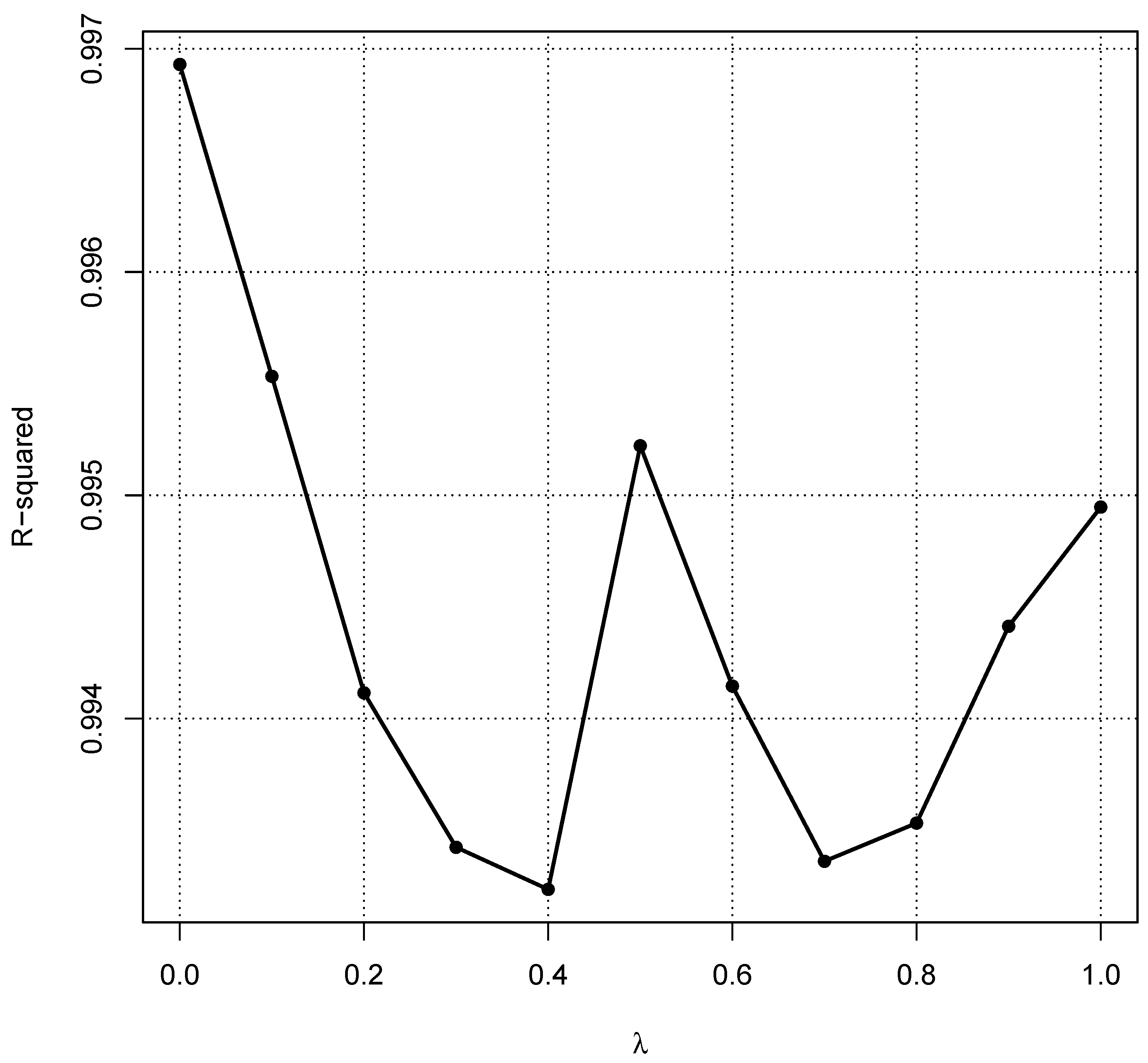
4.4. Choice of $\lambda$

In Section 4.1, Section 4.2 and Section 4.3, it was assumed that all measured values and the $\mathrm{LOD}$ were already Box–Cox-transformed in such a way that the transformed values from the healthy population follow a normal distribution. As mentioned before, the original version of reflimR, which cannot handle values below the $\mathrm{LOD}$, uses Bowley’s quartile skewness of all data to decide whether the values from the healthy population follow a normal or a log-normal distribution. Bowley’s quartile skewness cannot be computed when the 25 percentile is below the $\mathrm{LOD}$, so that it is not suitable for a general approach tolerating values below the $\mathrm{LOD}$. According to [14], it might be reasonable to assume that the values from the healthy population follow a log-normal distribution. This issue will be discussed in more detail in Section 6.2.

An alternative approach is to try out different values for $\lambda$ and choose the “most suitable” value. There are different ways to select the most suitable value for $\lambda$, which are illustrated below using a synthetic data set generated as follows.

• The healthy population follows a log-normal distribution with parameters $\mu =0$ and $\sigma =0.5$, i.e., the log-values follow a normal distribution with expected value $\mu =0$ and standard deviation $\sigma =0.5$.
• $\mathrm{LOD}=0.7$ is chosen, so that almost 25% of the healthy population have values below the $\mathrm{LOD}$.
• Values from a pathological population are added following a log-normal distribution with parameters $\mu =3$ and $\sigma =3$ for the associated normal distribution.
• Altogether, 500 values are generated, 400 from the healthy population and 100 from the pathological population.

The theoretical reference interval is in this case $[0.375,2.664]$. The synthetic data set contains 98 values below $\mathrm{LOD}$. The mixed distribution of the healthy and pathological values above the $\mathrm{LOD}$ is shown in Figure 1 on the original scale (left) and on a logarithmic scale (right).

If one enforces a logarithmic transformation for the application of truncMod, the maximum likelihood approach estimates the reference interval—after applying the inverse transformation—as $[0.381,2.690]$, whereas the quantile-based approach yields $[0.386,2.657]$. The estimated reference intervals for the maximum likelihood approach are shown in Figure 2 as $\lambda$ for the Box–Cox transformation, and it varies between 0 and 1 in steps of 0.1. The red line shows the estimates for the lower limit of the reference interval, while the blue line shows the estimates for the upper limit of the reference interval.

It can be seen clearly that the choices $\lambda =0$ and $\lambda =1$ lead to quite different reference intervals. Because we used synthetic data here, we know that $\lambda =0$ is the correct choice in this case. However, in the case of real data, this information is not available. One can inspect the histograms of the values remaining after truncation and the fitted distribution—i.e., the estimated normal distribution after the application of the corresponding inverse Box–Cox transformation. Figure 3 shows the respective histogram of the truncated data when $\lambda =0$ was chosen on the left. The red line indicates the corresponding fitted log-normal distribution. The result for $\lambda =1$ is shown on the right of Figure 3, where the red line shows the fitted normal distribution. It is obvious that the fit on the left is much better than the one on the right, indicating that $\lambda =0$ should be preferred over $\lambda =1$.

Quantile–Quantile plots offer another visualization for the comparison of the results for different values of $\lambda$. The values below the $\mathrm{LOD}$ are considered in the quantile–quantile plots by starting the x-axis with the corresponding quantile of the standard normal distribution defined by the (transformed) $\mathrm{LOD}$. Figure 4 shows the quantile–quantile plots of a standard normal distribution against the corresponding quantiles of the Box–Cox transformed values after truncation where the quantiles are already corrected for the truncation. The left quantile–quantile plot corresponds to $\lambda =0$, the right to $\lambda =1$. The red lines represent the fitted regression lines for the quantiles. It is evident that the regression line in the quantile–quantile plot for $\lambda =0$ fits better than the one for $\lambda =1$, speaking again in favor of the correct $\lambda =0$.

We also applied the Kolmogorov–Smirnov test to the truncated data shown in Figure 3, testing for the corresponding truncated log-normal distribution ($\lambda =0$) on the left and for the corresponding truncated normal distribution ($\lambda =1$), yielding a p-value of 0.81 for the case of the truncated log-normal distribution and a p-value < 0.00001 for the truncated normal distribution. This again indicated that $\lambda =0$ is a more appropriate choice than $\lambda =1$.

If one wants to compare more than two values of $\lambda$ at the same time, one can plot the coefficients of determination ($r^2$) for the regression lines in the quantile–quantile plots depending on $\lambda$. The corresponding $r^2$-values are depicted in Figure 5. The maximum is reached at the correct value of $\lambda =0$.

It should be noted that it is not meaningful to compare the likelihoods of the maximum likelihood estimators for different values of $\lambda$ because the number of values for the likelihood computation depends on the truncation on which $\lambda$ has a strong influence.

5. Analysis and Validation

This section is devoted to theoretical and simulation-based analyses of the proposed method and a validation using real data.

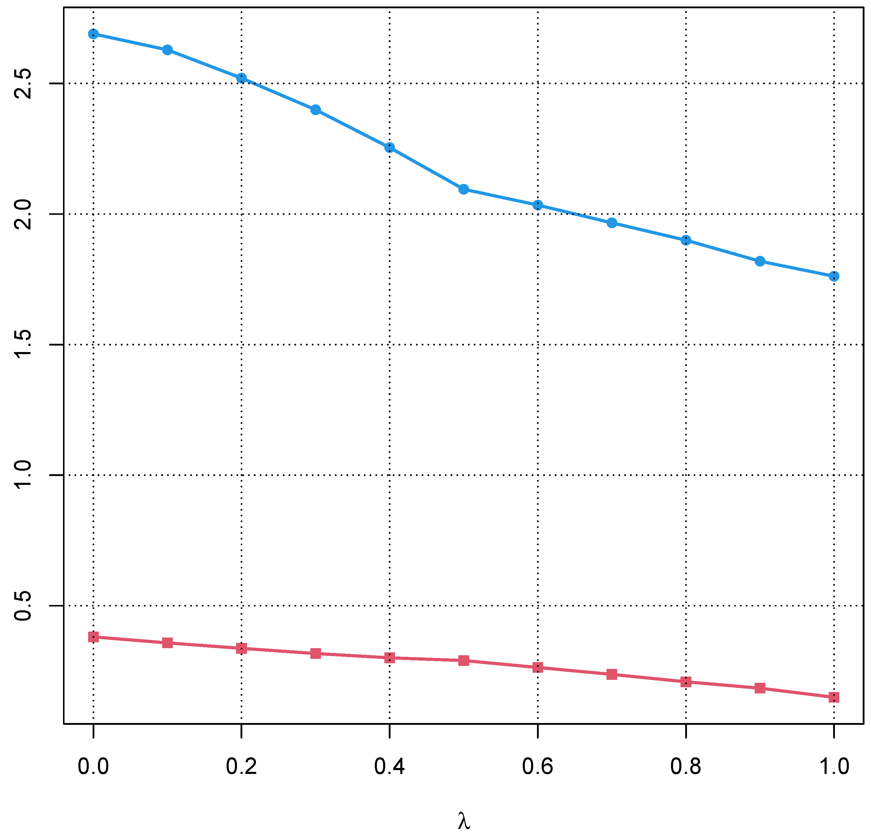
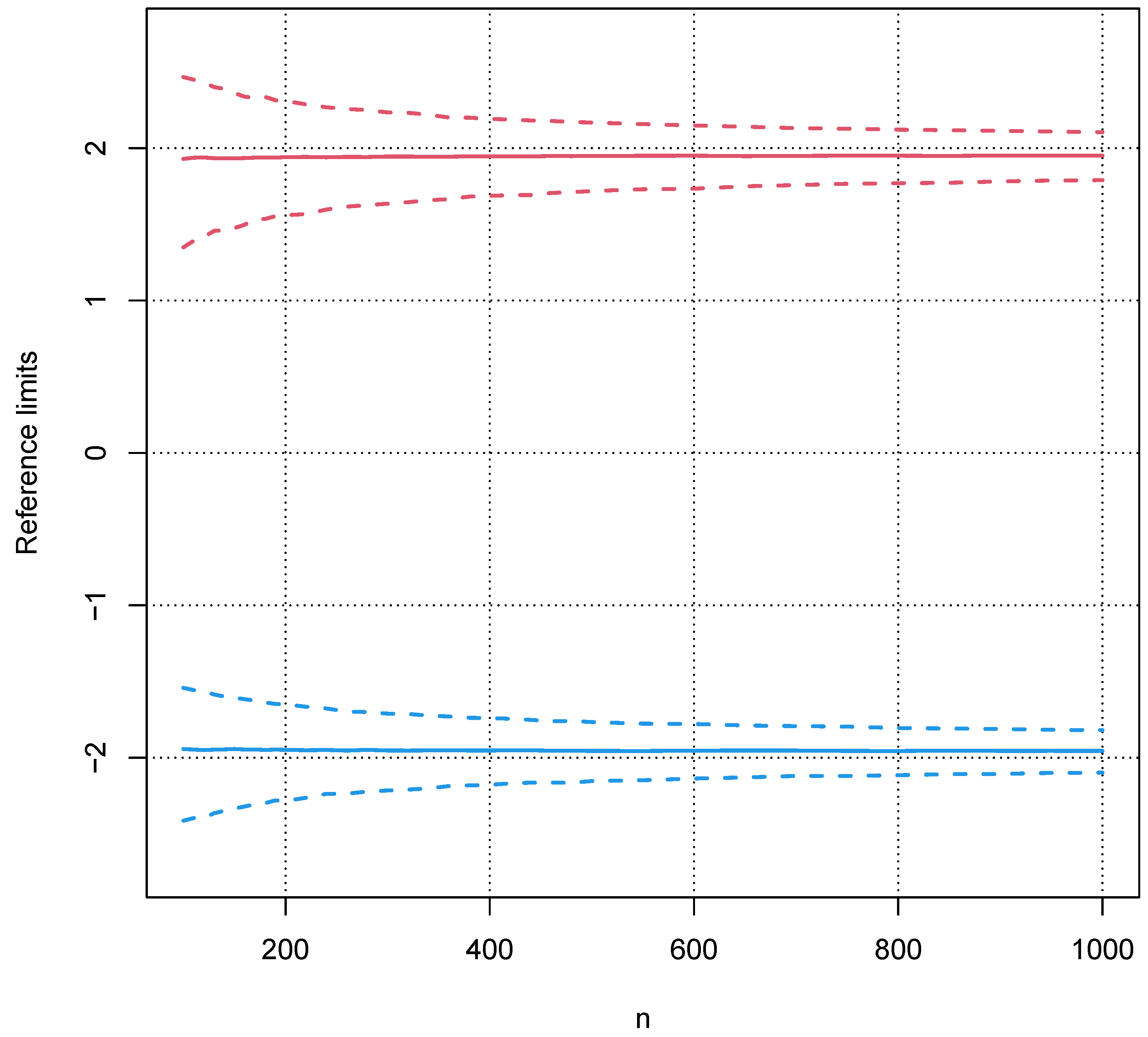
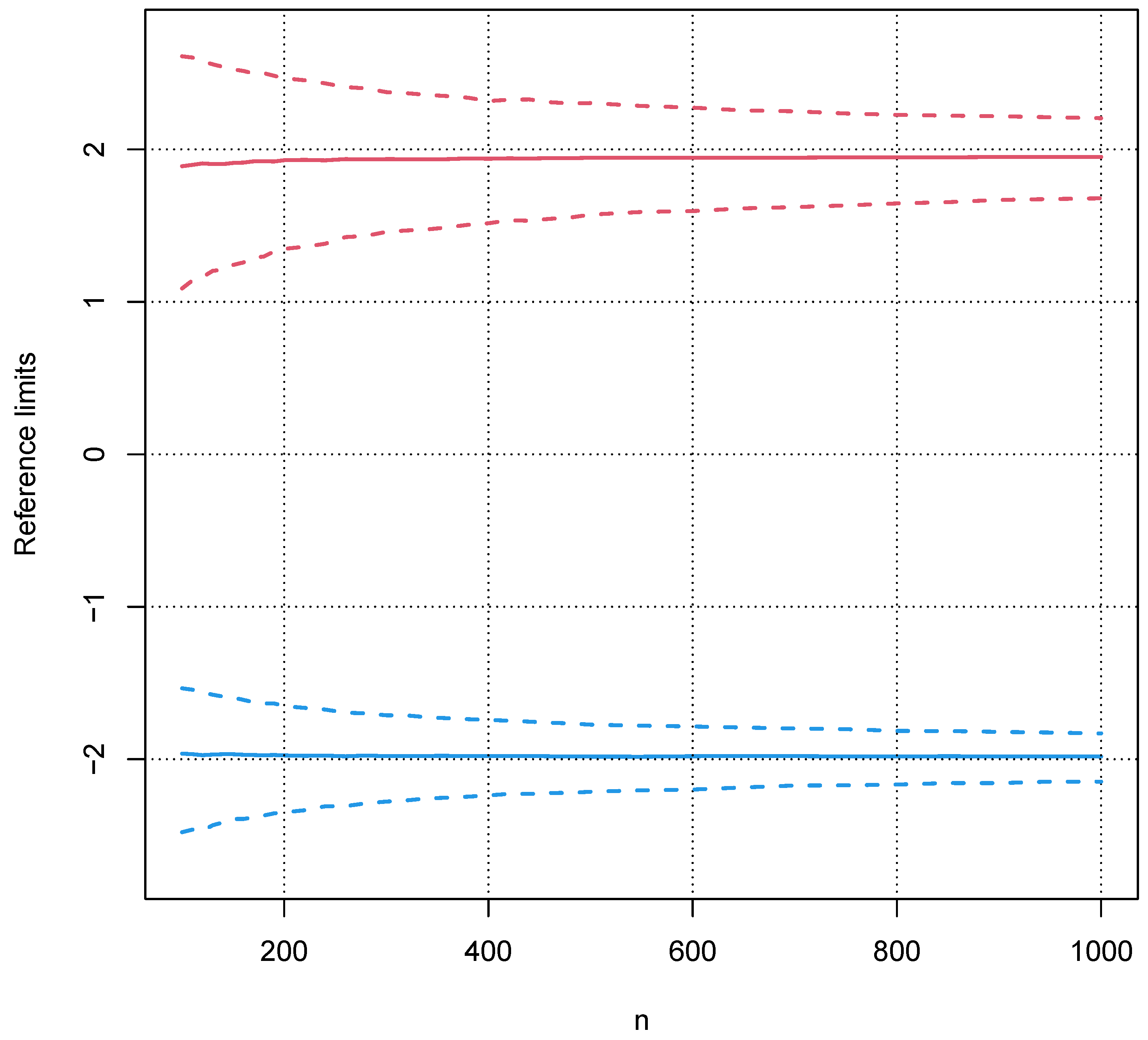
5.1. Bias of the Sample Interquartile Range

It is well known that the sample interquartile range is often a biased estimator for the interquartile range of a given theoretical distribution (see for example [17]). Our proposed truncation algorithm is based on the upper part of the interquartile range, specifically the difference between the third quartile and the median. We therefore carried out simulations for sample sizes ranging between 100 and 10,000. For each sample size, we generated a sample from a standard normal distribution with $\mathrm{LOD}={\mathsf{\Phi }}^{-1}\left(0.2\right)$ and estimated the reference interval with a quantile-based and maximum likelihood approach. This was repeated 1000 times for each sample size. The red line in Figure 6 shows the mean of the estimates of the upper reference limit for the maximum likelihood approach for each sample size. The theoretically correct value is ${\mathsf{\Phi }}^{-1}\left(0.975\right)\approx 1.96$. The dashed red lines mark the empirical 95% confidence band derived from the 1000 repetitions. The corresponding results for the lower reference limit are shown in blue.

Figure 7 presents the same information as Figure 6 but for the quantile-based approach described in Section 4.2.

It can be seen that both approaches tend to have a small bias for too narrow reference interval estimations for smaller sample sizes. The bias tends to vanish with larger sample sizes, indicating that while both estimators are biased, they seem to be Fisher consistent. The confidence bands for the maximum likelihood approach are slightly narrower than the ones for the quantile-based method, especially for the upper limit of the reference interval. The effect of narrower confidence bands for the maximum likelihood approach can also be observed for other values of the $\mathrm{LOD}$. The maximum likelihood approach becomes more efficient with a lower $\mathrm{LOD}$, i.e., with a decreasing number of values below the $\mathrm{LOD}$. This does not apply to the quantile-based approach, at least when the upper reference limit is considered. Although a bias correction could be based on large-scale Monte Carlo simulations, the bias correction would lead to no relevant improvement because the bias is very small compared with the uncertainty depending on the sample size. One can see that the uncertainty caused by the sample size is quite high for sample sizes below 200.

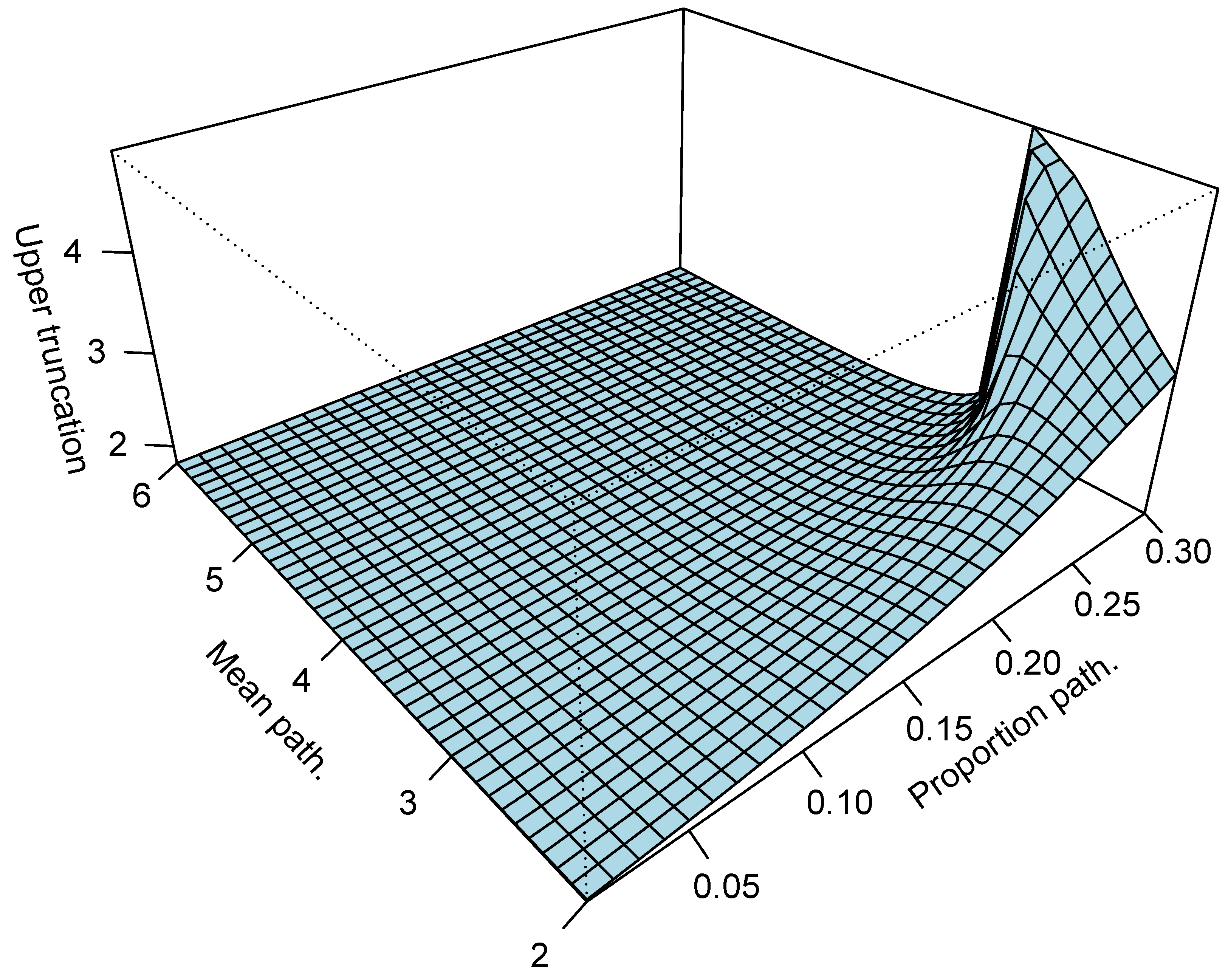
5.2. Influence of a Pathological Population on the Truncation Algorithm

The simulation results in the previous subsection have demonstrated that the truncation Algorithm 1 estimates the 97.5 percentile correctly for larger sample sizes if the sample contains no pathological values. We now investigate the influence of a pathological population on the truncation algorithm for large—or theoretically infinite—sample sizes.

Let $F\left(x\right)$ be the overall cumulative distribution function of healthy and pathological values. For $t>0$, $F_t\left(x\right)$ denotes the corresponding cumulative distribution function truncated at t, i.e.,

$$F_t\left(x\right)=\left\{\begin{array}{cc}{\displaystyle \frac{F\left(x\right)}{F\left(t\right)}}\hfill & \mathrm{if}x\le t,\hfill \\ 1\hfill & \mathrm{if}x>t.\hfill \end{array}\right.$$

(19)

If the iterative truncation algorithm has truncated the distribution at t in one of its steps, the truncation in the next step would be at

$$\tilde{t}=F_t^{-1}\left(0.5\right)+\left(F_t^{-1}\left(0.75\right)-F_t^{-1}\left(0.5\right)\right)·c$$

(20)

where $c={\displaystyle \frac{{\mathsf{\Phi }}^{-1}\left(0.975\right)}{{\mathsf{\Phi }}^{-1}\left(0.75\right)}}\approx 2.905847$. The truncation algorithm will converge when $\tilde{t}=t$ holds, i.e., for

$$t=F_t^{-1}\left(0.5\right)+\left(F_t^{-1}\left(0.75\right)-F_t^{-1}\left(0.5\right)\right)·c.$$

(21)

For $0<\alpha <1$, the $\alpha$ quantile $x_{\alpha }=F_t^{-1}\left(\alpha \right)$ for the truncated distribution can be rewritten using Equation (19) and $F_t\left(x_{\alpha }\right)=\alpha$ as follows:

$$x_{\alpha }=F^{-1}(0.5·F\left(t\right))+\left(F^{-1}(0.75·F\left(t\right))-F^{-1}(0.5·F\left(t\right))\right)·c,$$

(22)

so that Equation (21) becomes

$$t=F^{-1}(0.5·F\left(t\right))+\left(F^{-1}(0.75·F\left(t\right))-F^{-1}(0.5·F\left(t\right))\right)·c.$$

(23)

Given a cumulative distribution function $F\left(x\right)$, this non-linear equation can be solved numerically by a simple bisection method. The same applies to the computation of the quantile function $F^{-1}\left(\alpha \right)$. Given the overall cumulative distribution of the healthy and pathological population, we can therefore compute the theoretical truncation result t of Algorithm 1, corresponding to the result for a very large sample size.

It should be noted that the choice of the $\mathrm{LOD}$ has no influence on the truncation algorithm as long as the median of the truncated distribution is larger than the $\mathrm{LOD}$.

To investigate the influence of pathological values on the truncation algorithm, we consider the following configuration. Without a loss of generality, the (transformed) values of the healthy sub-population follow a standard normal distribution. In most cases in laboratory medicine, both sub-populations would follow log-normal distributions, and we consider the already transformed data here. The (transformed) values of the pathological sub-population are assumed to follow a normal distribution with expected value $\mu$ and standard deviation $\sigma =1$. The mixed distribution of the healthy and pathological population is then

$$F\left(x\right)=(1-\alpha )·\mathsf{\Phi }\left(x\right)+\alpha ·\mathsf{\Phi }(x-\mu )$$

(24)

where $\alpha$ is the proportion of pathological cases. We solve Equation (21) for $\mu \in [2,6]$ and $\alpha \in [0,0.3]$. Figure 8 shows the truncation point that Algorithm 1 would yield for an infinite sample size. The correct targeted truncation point for the healthy sub-population is ${\mathsf{\Phi }}^{-1}\left(0.975\right)\approx 1.96$. It can be seen that as long as the pathological population does not overlap too much with the healthy population, i.e., $\mu >3$, the pathological values have almost no influence on the correct estimation of the truncation limit, even when 30% of the values are pathological. If there is a strong overlap between the healthy and the pathological population, i.e., $\mu <3$, only a smaller proportion of pathological values can be tolerated without spoiling the estimation of the truncation limit. For $\mu =2$, more than 15% of pathological values cause the estimated upper reference limit to deviate too much from the true value. This observation is very much in accordance with the results presented in Figure 2 provided in [18] where, however, the problem of values below the $\mathrm{LOD}$ was not considered.

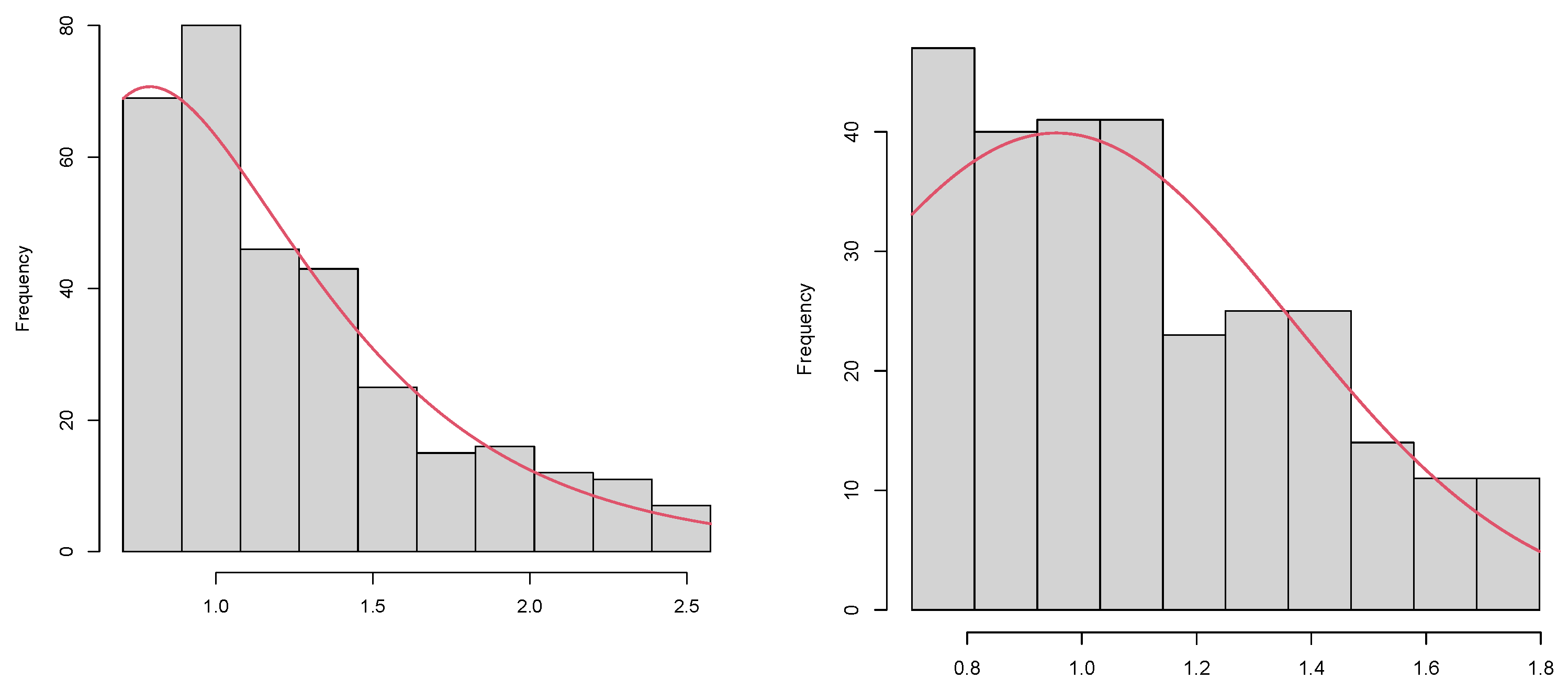
5.3. Validation with Real Data

We validate our approach with real laboratory data from the German Heart Center in Munich. We deliberately chose an analyte where no values below the $\mathrm{LOD}$ are observed in order to have a “ground truth” with which we compare our results. We first compute the reference interval with state-of-the-art indirect methods, i.e., with refineR [6], reflimR [3], and with a Gaussian mixture model [19] based on a similar idea as [10] using all values. We then define artificial levels of detection and apply our maximum likelihood approach.

We chose to focus our analysis on young men between the ages of 20 and 30 as the number of pathological values in this group remained manageable. In older age groups, the prevalence of myocardial infarctions, which elevates CK levels, increases significantly, complicating the interpretation of the reference limits. For the experiment, we artificially set the LOD for CK at 50, 75, and 100 U/L, resulting in LOD proportions of 4.5%, 18%, and 40%, respectively, relative to the presumably non-pathological values.

The data set contains 888 measurements of CK values ranging between 25 and 997.

Table 1. Estimated reference intervals for CK. The first columns specifies the methods where reflimLOD.Quant and reflimLOD.MLE stand for the quantile-based and the maximum likelihood approach introduced in Section 4.2 and Section 4.3, respectively. The lower and upper limit of the reference intervals are shown in the second and third column, respectively. The artificially introduced value for the $\mathrm{LOD}$ is given in the fourth column. The number of values below the $\mathrm{LOD}$ is denoted in the last column.

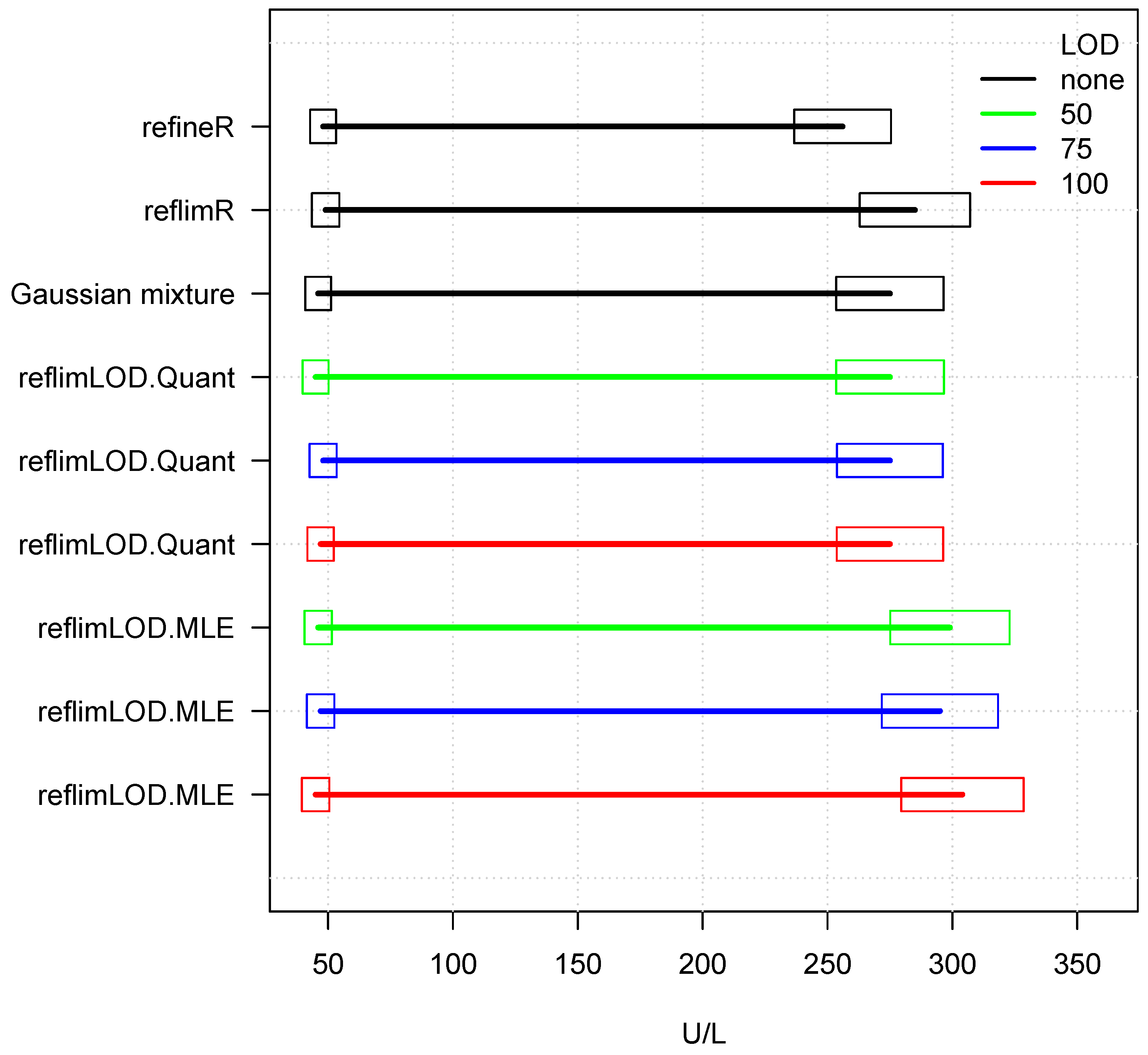
Method	Lower Limit	Upper Limit	$\mathbf{LOD}$	No. of Values $<\mathbf{LOD}$
refineR	48	256	0	0
reflimR	49	285	0	0
Gaussian mixture	46	275	0	0
reflimLOD.Quant	45	275	50	33
reflimLOD.Quant	48	275	75	132
reflimLOD.Quant	47	275	100	296
reflimLOD.MLE	46	299	50	33
reflimLOD.MLE	47	295	75	132
reflimLOD.MLE	45	304	100	296

shows the result of state-of-the-art indirect methods that cannot handle values below the $\mathrm{LOD}$ and our approach for different values for an artificial $\mathrm{LOD}$ value. It can be seen that the estimated reference intervals are quite consistent. Our maximum likelihood approach introduced in Section 4.3 yields very concordant estimates, even when more than one third of the values are below the $\mathrm{LOD}$.

The estimated reference intervals remain consistent with respect to permissible differences computed on the basis of the method proposed in [20]. Figure 9 shows the corresponding reference intervals with permissible differences as boxes for each of the methods listed in Table 1.

The estimation of the upper reference limit is independent of the $\mathrm{LOD}$ value for reflimLOD.Quant because the truncation boundary from Algorithm 1 is used directly as the estimate for the upper reference limit. Algorithm 1 derives the truncation iteratively based on the median and the third quartile, which are not influenced by the $\mathrm{LOD}$ value as long as there are less than 50% of the values below the $\mathrm{LOD}$.

6. Conclusions and Discussion

We have introduced an indirect method for reference interval estimation called reflimLOD with two variants reflimLOD.Quant and reflimLOD.MLE that can cope with a substantial proportion of values below the $\mathrm{LOD}$, provided that the median of the healthy population is above the $\mathrm{LOD}$. The documented R code is available in the Supplementary Materials.

6.1. Conclusions

The possibility to compute reference intervals in the presence of values below the $\mathrm{LOD}$ offers various advantages. Firstly, it allows for the estimation of the upper limit of the reference interval to identify possible pathological values. Additionally, the lower limit of the reference interval, even if it falls below the the $\mathrm{LOD}$, is of interest because standardization methods for laboratory values like the so-called zlog value [21] require both a defined lower and an upper limit of the reference interval.

In contrast to the modified TMC method [7], reflimLOD is publicly available in the Supplementary Materials. Further advantages are that reflimLOD, like reflimR, only requires fractions of a second to calculate reference limits and delivers reproducible results with sample sizes of a few hundred values [3]. TMC, on the other hand, like all methods based on $\lambda$ estimation, requires calculation times in the order of one minute and a sample size of at least 1000 values [3,12,22].

6.2. Discussion

This paper deals with a primarily medical problem, viewed from a statistical perspective. Therefore, the discussion is divided into a statistical part, which explains the advantages and limitations of the algorithm presented here, and a medical part, in which we describe its practical utility for the interpretation of laboratory values.

Our proposed truncation algorithm is based on the median and the third quartile. The two quartiles could be replaced by any other two quantiles. Of course, Equations (5)–(11) have to be modified accordingly. The larger the range between the two selected quantiles, the better the estimation when no pathological values are present, and the smaller quantile remains over the $\mathrm{LOD}$. The median seems to be a good compromise for the smaller quantile for the truncation algorithm. It allows up to 50% of the values to be below the $\mathrm{LOD}$ from the healthy population but still includes the peak of the distribution of the non-pathological values. Replacing the third quartile by a larger quantile would increase the danger where pathological values gain influence on the truncation algorithm. A smaller quantile than the third quartile would increase the variance of the estimator and could lead to high uncertainty in the estimates, especially for smaller data sets. This is why we recommend to stay with the choice of the median and the third quartile.

Apart from a purely statistical analysis, it is important to view our approach from a medical point of view. For the correct interpretation of laboratory results, it is essential that several kinds of limits and intervals have been defined [23]. Reference intervals consisting of a lower and an upper reference limit help to decide whether a value should be interpreted as “normal” or “pathological” [2], tolerance intervals around each reference limit indicate which deviation from a comparative target value is medically relevant [20], and decision limits are aids in determining the probability of a specific diagnosis or risk [24]. In this paper, we mainly deal with the first issue and mention the second in the context of Table 1, where we ask whether the reference limits obtained with our algorithm agree sufficiently well with those from three standard methods.

With this information in mind, the algorithm proposed here solves a statistical problem that is relevant to laboratory medicine but has rarely been addressed from a statistical perspective. The only publication, to the best of our knowledge, is that of Haeckel et al. [7] describing the estimation of the lower reference limit for troponin measurements with a high proportion of values below the analytical detection level $\mathrm{LOD}$.

However, missing lower limits for reference intervals are a frequent phenomenon in the method specifications stored in laboratory information systems, i.e., there are only upper limits such as “creatin kinase < 170 U/L” or “bilirubin < 1.2 mg/dL”. In most cases, this is outdated information from a time when analytical methods were not as sensitive as they are today. A frequent reason for an apparent lack of a lower reference limit is that the specified value is not an upper reference limit but a decision limit, for example a maximally acceptable LDL cholesterol value [25] or a desirable minimum vitamin D level [26].

The phenomenon we are dealing with here concerns the first of the two reasons with a focus on cases where the analyte under investigation is present in such low concentrations that it cannot (yet) be completely detected by the analytical methods currently available. For the cardiac marker creatine kinase (CK), which we have deliberately chosen as an example here, this no longer applies today, but for the cardiac marker troponin investigated by Haeckel et al. [7], the analytical sensitivity is actually not sufficient to quantitatively determine “low normal” levels [27]. Another example of an analyte affected by this sensitivity issue is the use of the inflammation marker C-reactive protein (CRP) for the assessment of the cardiovascular risk [28]. Many newer biomarkers such as cytokines, hormones, neurotransmitters, or tumor markers also fall into this category.

The establishment of a lower reference limit is not only desirable for the comprehensive interpretation of laboratory results in clinical practice, but also has an impact on the calculation of tolerance intervals (see above) and on the standardization of laboratory values, e.g., for data storage in electronic health records [21] or for machine learning [29]. In both cases, the underlying calculations require the log-transformation of the original reference limits, which is impossible if the lower limit is zero (or undefined).

Because we do not have any information on whether there are diseases with analyte levels below the (unmeasurable) lower reference limit, it seems appropriate to exclude such pathological conditions in our statistical model (see problem formulation in Section 2). In the case of CK, which is used here as an example, the Gaussian mixture modelling approach actually yielded two plausible fractions (normal and elevated results), with no indication of a relevant third fraction containing pathologically low values. From a physiological point of view, there is no reason why a genetic or acquired deficiency of such an essential enzyme of energy metabolism could be compatible with life. The same applies to the troponins, which are pivotal regulators of heart contraction and relaxation [30].

References

- Horowitz, G.; Altaie, S.; Boyd, J.C.; Ceriotti, F.; Garg, U.; Horn, P.; Pesce, A.; Sine, H.E.; Zakowski, J. Defining, Establishing, and Verifying Reference Intervals in the Clinical Laboratory; Tech Rep Document EP28-A3C; Clinical & Laboratory Standards Institute: Wayne, PA, USA, 2010. [Google Scholar]
- Jones, G.; Haeckel, R.; Loh, T.; Sikaris, K.; Streichert, T.; Katayev, A.; Barth, J.; Ozarda, Y. Indirect methods for reference interval determination: Review and recommendations. Clin. Chem. Lab. Med. 2018, 57, 20–29. [Google Scholar] [CrossRef] [PubMed]
- Hoffmann, G.; Klawitter, S.; Trulson, I.; Adler, J.; Holdenrieder, S.; Klawonn, F. A novel tool for the rapid and transparent verification of reference intervals in clinical laboratories. J. Clin. Med. 2024, 13, 4397. [Google Scholar] [CrossRef]
- Ichihara, K.; Boyd, J.C. IFCC Committee on Reference Intervals and Decision Limits (C-RIDL). An appraisal of statistical procedures used in derivation of reference intervals. Clin. Chem. Lab. Med. 2010, 48, 1537–1551. [Google Scholar] [CrossRef] [PubMed]
- Sikaris, K. Separating disease and health for indirect reference intervals. J. Lab. Med. 2021, 45, 55–68. [Google Scholar] [CrossRef]
- Ammer, T.; Schützenmeister, A.; Prokosch, H.U.; Rauh, M.; Rank, C.M.; Zierk, J. refineR: A Novel Algorithm for Reference Interval Estimation from Real-World Data. Sci. Rep. 2021, 11, 16023. [Google Scholar] [CrossRef] [PubMed]
- Haeckel, R.; Wosniok, W.; Torge, A.; Junker, R. Reference limits of high-sensitive cardiac troponin T indirectly estimated by a new approach applying data mining. A special example for measurands with a relatively high percentage of values at or below the detection limit. J. Lab. Med. 2021, 45, 87–94. [Google Scholar] [CrossRef]
- Yeo, I.-K.; Johnson, R.A. A new family of power transformations to improve normality or symmetry. Biometrika 2000, 87, 954–959. [Google Scholar] [CrossRef]
- Wosniok, W.; Haeckel, R. A new indirect estimation of reference intervals: Truncated minimum chi-square (TMC) approach. Clin. Chem. Lab. Med. 2019, 57, 1933–1947. [Google Scholar] [CrossRef]
- Concordet, D.; Geffré, A.; Braun, J.P.; Trumel, C. A new approach for the determination of reference intervals from hospital-based data. Clin. Chim. Acta 2009, 405, 43–48. [Google Scholar] [CrossRef]
- Scott, D.W. Averaged shifted histogram. WIREs Comput. Stat. 2010, 2, 160–164. [Google Scholar] [CrossRef]
- Klawonn, F.; Riekeberg, N.; Hoffmann, G. Importance and uncertainty of λ-estimation for Box-Cox transformations to compute and verify reference intervals in laboratory medicine. Stats 2024, 7, 172–184. [Google Scholar] [CrossRef]
- Bowley, A.L. Elements of Statistics; P.S. King & Son: London, UK, 1901. [Google Scholar]
- Haeckel, R.; Wosniok, W. Observed, unknown distributions of clinical chemical quantities should be considered to be log-normal: A proposal. Clin. Chem. Lab. Med. 2010, 48, 1393–1396. [Google Scholar] [CrossRef] [PubMed]
- Nelder, J.A.; Mead, R. A simplex algorithm for function minimization. Comput. J. 1965, 7, 308–313. [Google Scholar] [CrossRef]
- R Core Team. R: A Language and Environment for Statistical Computing; R Foundation for Statistical Computing: Vienna, Austria, 2023. [Google Scholar]
- Whaley, D.L. The Interquartile Range: Theory and Estimation. Electronic Theses and Dissertations. Master’s Thesis, East Tennessee State University, Johnson City, TN, USA, 2005. Paper 1030. Available online: https://dc.etsu.edu/etd/1030 (accessed on 7 July 2024).
- Zierk, J.; Arzideh, F.; Kapsner, L.A.; Prokosch, H.-U.; Metzler, M.; Rauh, M. Reference interval estimation from mixed distributions using truncation points and the Kolmogorov-Smirnov distance (kosmic). Sci. Rep. 2020, 10, 1704. [Google Scholar] [CrossRef] [PubMed]
- Hoffmann, G.; Allmeier, N.; Kuti, M.; Holdenrieder, S.; Trulson, I. How Gaussian mixture modelling can help to verify reference intervals from laboratory data with a high proportion of pathological values. J. Lab. Med. 2024, 48, 251–258. [Google Scholar] [CrossRef]
- Haeckel, R.; Wosniok, W.; Arzideh, F. Equivalence limits of reference intervals for partitioning of population data. Relevant differences of reference limits. LaboratoriumsMedizin 2016, 40, 199–205. [Google Scholar] [CrossRef]
- Hoffmann, G.; Klawonn, F.; Lichtinghagen, R.; Orth, M. The zlog value as a basis for the standardization of laboratory results. J. Lab. Med. 2017, 41, 20170135. [Google Scholar] [CrossRef]
- Anker, S.; Morgenstern, J.; Adler, J.; Brune, M.; Brings, S.; Fleming, T.; Kliemank, E.; Zorn, M.; Fischer, A.; Szendroedi, J.; et al. Verification of sex- and age-specific reference intervals for 13 serum steroids determined by mass spectrometry: Evaluation of an indirect statistical approach. Clin. Chem. Lab. Med. 2023, 61, 452–463. [Google Scholar] [CrossRef]
- Ozarda, Y.; Sikaris, K.; Streichert, T.; Macri, J. Distinguishing reference intervals and clinical decision limits—A review by the IFCC committee on reference intervals and decision limist. Crit. Rev. Clin. Lab. Sci. 2018, 55, 420–431. [Google Scholar] [CrossRef]
- Ceriotti, F.; Henny, J. Are my laboratory results normal? Considerations to be made concerning reference intervals and decision limits. EJIFCC 2008, 19, 106–114. [Google Scholar]
- Virani, S.S.; Aspry, K.; Dixon, D.L.; Ferdinand, K.C.; Heidenreich, P.A.; Jackson, E.J.; Jacobson, T.A.; McAlister, J.L.; Neff, D.R.; Gulati, M.; et al. The importance of low-density lipoprotein cholesterol measurement and control as performance measures: A joint Clinical Perspective from the National Lipid Association and the American Society for Preventive Cardiology. J. Clin. Lipidol. 2023, 17, 208–218. [Google Scholar] [CrossRef]
- Rebelos, E.; Tentolouris, N.; Jude, E. The role of vitamin D in health and disease: A narrative review on the mechanisms linking vitamin D with disease and the effects of supplementation. Drugs 2023, 83, 665–685. [Google Scholar] [CrossRef]
- Lazar, D.R.; Lazar, F.-L.; Homorodean, C.; Cainap, C.; Focsan, M.; Cainap, S.; Olinic, D.M. High-sensitivity troponin: A review on characteristics, assessment, and clinical implications. Dis. Markers 2022, 2022, 9713326. [Google Scholar] [CrossRef]
- Helfenstein Fonseca, F.A.; de Oliveira Izar, M.C. High-sensitivity C-reactive protein and cardiovascular disease across countries and ethnics. Clinics 2016, 71, 235–242. [Google Scholar] [CrossRef]
- Al-Mekhlafi, A.; Klawitter, S.; Klawonn, F. Standardization with zlog values improves exploratory data analysis and machine learning for laboratory data. J. Lab. Med. 2024, 48, 215–222. [Google Scholar] [CrossRef]
- Cheng, Y.; Regnier, M. Cardiac troponin structure-function and the influence of hypertrophic cardiomyopathy associated mutations on modulation of contractility. Arch. Biochem. Biophys. 2017, 601, 11–21. [Google Scholar] [CrossRef]