Model Validation of a Single Degree-of-Freedom Oscillator: A Case Study

Abstract

In this paper, we investigate a validation process in order to assess the predictive capabilities of a single degree-of-freedom oscillator. Model validation is understood here as the process of determining the accuracy with which a model can predict observed physical events or important features of the physical system. Therefore, assessment of the model needs to be performed with respect to the conditions under which the model is used in actual simulations of the system and to specific quantities of interest used for decision-making. Model validation also supposes that the model be trained and tested against experimental data. In this work, virtual data are produced from a non-linear single degree-of-freedom oscillator, the so-called oracle model, which is supposed to provide an accurate representation of reality. The mathematical model to be validated is derived from the oracle model by simply neglecting the non-linear term. The model parameters are identified via Bayesian updating. This calibration process also includes a modeling error due to model misspecification and modeled as a normal probability density function with zero mean and standard deviation to be calibrated.

1. Introduction

Quantifying uncertainty is a problem common to scientists dealing with mathematical models of physical processes. There are a wide range of numerical methods to solve systems of ordinary differential equations, such as the Euler method, higher-order Taylor methods, and Runge–Kutta methods. For systems of partial differential equations, we consider several numerical methods, such as finite difference, finite element, finite volume, and spectral methods to produce solutions to physical models based on differential equations. If numeral methods are used, the resulting solution is an approximation to the true underlying solution and usually consists of a single solution set when parameter and starting values are known and specified. However, in many processes there exist various sources of noise to the process. Aleatoric uncertainty is an “external error” which may take the form of measurement error or some other error associated with generating the solution. The key to external (Aleatoric) error is that the error exists on the solution set. Epistemic uncertainty is model uncertainty/misspecification uncertainty which exists in the formulation of the model. This can be a result of not accounting for various components of a model. Epistemic uncertainty can be considered “internal error” as it exists before the solution to the differential equation is generated. For a very good overview of Bayesian model calibration, see [1], as it addresses many of the issues associated when quantifying uncertainty for computer models, while, for quantifying uncertainty for differential equations models, see [2]. For a good reference for techniques dealing with model inadequacy, see [3], and for work on model misspecification and model order see [4].

These two different types of uncertainty are manifested in different ways. For example, external error is manifested by unstructured random noise about the solution set. In contrast, internal error is propagated through the differential equation solver and may manifest itself as structured changes in the solution set which is called uncertainty propagation [5]. To highlight this issue consider the simple differential equation with no uncertainty introduced:

$$\frac{\delta P}{\delta t}=kP$$

(1)

this has the well known solution with initial condition $P_0$:

$$P\left(t\right)=P_0{e}^{kt}$$

(2)

To account for external error the solution to Equation (1) would be:

$$P\left(t\right)=P_0{e}^{kt}+ϵ\left(t\right)$$

(3)

where $ϵ\left(t\right)$ follows some appropriate probability distribution. However, if we have internal error then Equation (1) would be:

$$\frac{\delta Q}{\delta t}=kQ+\xi \left(t\right)$$

(4)

where $\xi \left(t\right)$ follows some appropriate probability distribution. Let $Q\left(t\right)$ be the solution to Equation (1), then if an external error is added to the model we have $N\left(t\right)=Q\left(t\right)+ϵ\left(t\right)$, where $ϵ\left(t\right)$ follows some appropriate probability distribution. One can see the effects of both types of errors in Figure 1.

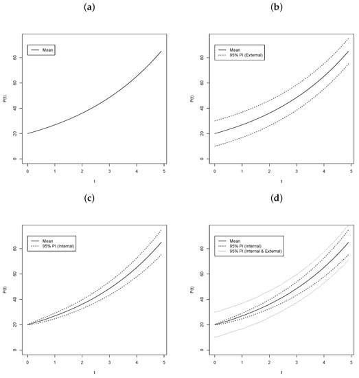
Figure 1. Trajectoriesfor simple population growth equation with: No Error (a), External Error (b), Internal Error (c), and Internal and External Error (d).

To construct the plots in Figure 1, simulation was used to ensure that the error structure was correctly represented, using 10,000 simulations. In panel (a) of Figure 1, the trajectory for an exponential growth model with $k=0.3$ and $P_0=20$, which contains no error. This subfigure shows exactly what one would expect. For panel (b), the exponential growth model with $k=0.3$ with external error $ϵ\left(t\right)\sim N(0,5)$. Notice that the error bands are virtually equidistant from the mean line. For panel (c), the exponential growth model the $k=0.3$ with internal error $\xi \left(t\right)\sim N(0,3)$ is plotted. In contrast to the external error only model the error bands increase in width as the time increases. Panel (d) shows the internal error $\xi \left(t\right)\sim N(0,3)$ with external error $ϵ\left(t\right)\sim N(0,5)$ added to it. Notice that the internal plus external error is not simply and addition of the two error as might think. This phenomenon is our motivation for this research.

The question we focus on here is can a model be purposely misspecified in order to improve computation time while still accounting for uncertainty induced due to this misspecification? Model misspecification is an important question especially when using deterministic models as they are typically assumed to be correct [6]. To approach this problem the Bayesian framework will be used from a fully Bayesian perspective [7,8] as it allows for a natural method to quantify uncertainty from different sources.

Notation

We have two major steps producing attributes, e.g., forcing, displacement, velocity and acceleration. All attributes in the training step will be denoted by superscript $\mathcal{T}$ while attributes in the validation step will not have any superscript. In each of the major step we have four different sets of attributes:

• The true unobserved attributes u, v, a produced by the system; i.e., the solution of the non-oracle differential equation using the true parameters $\theta$, forcing f and no internal or external errors. This is our target.
• The observed attributes $\overline{u}$, $\overline{v}$, $\overline{a}$ produced by the system; i.e., the solution of the non-oracle differential equation using the true parameters $\theta$ and the true forcing f with true external and internal errors added. This together with the forcing $\overline{f}$ are our data.
• The fitted/predicted attributes $\widehat{u}$, $\widehat{v}$, $\widehat{a}$, defined as the solution of either the oracle or non-oracle differential equation using estimated parameters $\widehat{\theta }$, $\overline{f}$ with predicted external and internal errors added.
• Attributes $\tilde{u}$, $\tilde{v}$, $\tilde{a}$ that are the solution of the oracle or non-oracle differential equation using estimated parameters $\widehat{\theta }$ with predicted internal and no external error added. These will be used for estimation of maximum.

2. Models

Suppose that the dynamics of a given system be modeled by an abstract initial-value problem:

$$F\left(t,u,\dot{u},\ddot{u},\dots ,u^{\left(n\right)}\right)=0,\forall t\in (0,T)$$

(5)

with appropriate boundary conditions, where $u^{\left(n\right)}$ denotes the $n^{\mathrm{th}}$ derivative of u with respect to the time variable t. Furthermore, we suppose that the function $F(t,u,\dot{u},\dots ,u^{\left(n\right)})$ can be separated into lower- and higher-order dynamics, G and H, respectively, such as:

$$F(t,u,\dot{u})=G(t,u,\dot{u},\dots ,u^{(\ell )})+H(t,u,\dot{u},\dots ,u^{\left(n\right)}),\forall t\in (0,T)$$

(6)

for some ℓ smaller than or equal to n and assume that the higher-order term H has smaller effects than the lower-order term for some values of the input parameters of the model. Due to the added complexity and computational cost associated with the solution of the higher-order dynamics model, one may want to introduce a misspecified model by retaining the lower-order dynamics in the following manner:

$$G(t,u,\dot{u},\dots ,u^{(\ell )})+ϵ\left(t\right)=0,\forall t\in (0,T)$$

(7)

where $ϵ\left(t\right)$ is a random process governed by some probability distribution with mean 0 and variance ${\sigma }_{ϵ}^2$. This model ignores the additional complexity of full model but accounts for the associated uncertainty through $ϵ$. In the following, we consider a non-linear single degree-of-freedom oscillator as the full model, which we will hereafter refer to as the oracle model, and a linear single degree-of-freedom oscillator as the misspecified model.

2.1. Non-Linear Single Degree-of-Freedom Oscillator

The displacement $u=u\left(t\right)$ around the equilibrium position of a non-linear single degree-of-freedom oscillator is governed by:

$$\begin{array}{cc}\hfill m\ddot{u}+\gamma \dot{u}+\left(k_l+k_n{u}^2\right)u=f\left(t\right)& \mathrm{in}(0,T)\hfill \\ \hfill u=u_0& \mathrm{at}t=0\hfill \\ \hfill \dot{u}=v_0& \mathrm{at}t=0\hfill \end{array}$$

(8)

where $\dot{u}$ denotes the time-derivative of u, $k_l$ is the linear component of the spring stiffness coefficient, $k_n$ is the higher-order component of spring stiffness, m is the mass of the object attached to the spring, and $\gamma$ is the damping coefficient. Moreover, the system is subjected to the external forcing $f=f\left(t\right)$ and initial displacement $u_0$ and velocity $v_0$.

A single degree-of-freedom oscillator is a popular model for modeling spring behavior. In an experimental setting, one can imagine that the spring be subjected to a sinusoidal forcing term by using a cam to apply a periodic and continuous force to the spring. From a mathematical point of view, any sufficiently smooth function can be represented as a Fourier series, in which case, the forcing term is given as a linear combination of trigonometric functions. In this work, the external forcing used in the generation of data for parameter identification will be chosen in the form:

$$f\left(t\right)=A_{c}sin\left(\frac{2\pi n_{c}t}{T}\right)$$

(9)

where $A_c$ is the amplitude and $n_c$ is an input parameter to control the angular frequency $\omega =2\pi n_c/T$ of the forcing term.

We also suppose that the external forcing $f\left(t\right)$ is subjected to unforeseen errors. These errors are collectively denoted by ${ϵ}_f$ such that the system is modeled by:

$$\begin{array}{cc}\hfill m\ddot{u}+\gamma \dot{u}+\left(k_l+k_n{u}^2\right)u+{ϵ}_f\left(t\right)=f\left(t\right)& \mathrm{in}(0,T)\hfill \\ \hfill u=u_0& \mathrm{at}t=0\hfill \\ \hfill \dot{u}=v_0& \mathrm{at}t=0\hfill \end{array}$$

(10)

In the following, we assume that above system is too complex to solve and has to be simplified in order to be tractable. Another point of view is that one does not necessarily know how to model all the physical phenomena occurring in the system.

2.2. Linear Single Degree-of-Freedom Oscillator

The model given in (10) can be decomposed into linear and non-linear components. Using the notation of (6), we have:

$$\begin{array}{cc}\hfill G(t,u,\dot{u},\ddot{u})& =m\ddot{u}+\gamma \dot{u}+k_{l}u-f\left(t\right)\hfill \end{array}$$

(11)

$$\begin{array}{cc}\hfill H(t,u,\dot{u},\ddot{u})& =k_n{u}^3\hfill \end{array}$$

(12)

with $n=2$ and $\ell =2$. Considering a model that retains the linear component, $G(t,u,\dot{u},\ddot{u})$, as defined in (11), and omitting the non-linear component, $H(t,u,\dot{u},\ddot{u})$, we arrive at the misspecified model:

$$\begin{array}{cc}\hfill m\ddot{u}+\gamma \dot{u}+k_{l}u+ϵ\left(t\right)=f\left(t\right)& \mathrm{in}(0,T)\hfill \\ \hfill u=u_0& \mathrm{at}t=0\hfill \\ \hfill \dot{u}=v_0& \mathrm{at}t=0\hfill \end{array}$$

(13)

Note that the variable $ϵ\left(t\right)$ in (13) accounts for both the model misspecification $H(t,u,\dot{u},\ddot{u})$ and errors ${ϵ}_f\left(t\right)$ in the forcing. Due to ${ϵ}_f\left(t\right)$ being governed by a probability distribution, then $ϵ\left(t\right)$ will also be governed by some probability distribution with some mean and variance ${\sigma }_{ϵ}^2$. In fact, the proposed formulation does not allow one to separate the uncertainty due to the non-linear component from possible errors when observing the forcing term. In other words, $ϵ$ can be viewed as a modeling error, “internal” to the system, in contrast to the traditional approach in which one considers an “external” error, to explain the error associated with the system solution. Finally notice, that if we fit Equations (10) and (13) to data, the estimated values of $\gamma$ and $k_l$ will be different depending on whether the cubic term is included or not.

In the following, the model defined in (10) will be referred to as the Oracle model and the misspecified model defined in (13) as the non-Oracle model. Figure 2 shows an example of sampled data for f versus u using forcing (9) with $A_c=5$ and ${\sigma }_{ϵ}=0.1$. As expected the data show a cubic relationship between displacement and forcing. The least squares estimated Oracle and non-Oracle models are overlaid on the data and show that the Oracle model fits extremely well the data while the non-Oracle model seems to provide a reasonable approximation. From a computational standpoint, the non-Oracle model is very appealing since its solution is far less computationally demanding than the Oracle model.

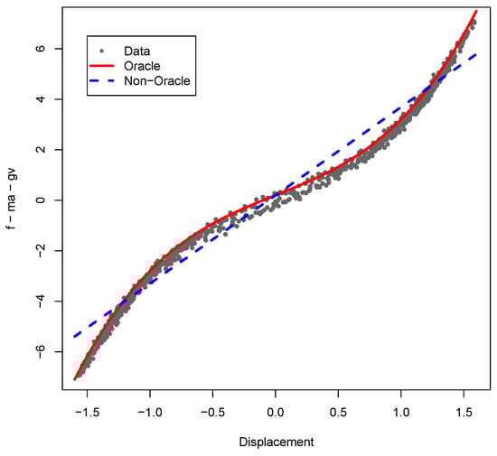
Figure 2. Force versus displacement with Oracle and non-Oracle models using forcing given by (9) with $A_c=5$ and centered Gaussian internal error with ${\sigma }_{ϵ}=0.1$.

Upon applying a force $f\left(t\right)$ to the system, we suppose that we can track the state of the system at times $t=t_0,t_1,\dots ,T$, which will result in the forcing vector $\mathbf{f}=(f_0,f_1,\dots ,f_T)$, internal errors $\mathit{\epsilon }=({ϵ}_0,{ϵ}_1,\dots ,{ϵ}_T$), as well as the solution vectors $\mathbf{u}=(u_0,u_1,...,u_T)$ for displacement, $\mathbf{v}=(v_0,v_1,\dots ,v_T)$ for velocity, and $\mathbf{a}=(a_0,a_1,\dots ,a_T)$ for acceleration. These unobserved quantities will be considered as a target for our estimation procedure. The solution vectors are actually observed contaminated with external errors and the observed solution vectors will be denoted by $\overline{\mathbf{u}}=({\overline{u}}_0,{\overline{u}}_1,\dots ,{\overline{u}}_T)$ for displacement, $\overline{\mathbf{v}}=({\overline{v}}_0,{\overline{v}}_1,\dots ,{\overline{v}}_T)$, for velocity and $\overline{\mathbf{a}}=({\overline{a}}_0,{\overline{a}}_1,\dots ,{\overline{a}}_T)$ for acceleration. These quantities will be referred to as data in our estimation procedure.

Figure 3 shows an example forcing (9) with ${\sigma }_{ϵ}=0$ (Panel a) and the resulting solutions of displacement (Panel b), velocity (Panel c), and acceleration (Panel d). Notice that the solutions for displacement are quite close in behavior with the non-Oracle model being somewhat smoother than the Oracle model. For velocity (Panel b), we observe that there is a marked difference between the Oracle and non-Oracle solutions. Specifically, the non-Oracle solutions do not fit well in the extremes and lack some dynamics exhibited by the Oracle model. The acceleration trajectories (Panel d) show that there is also a much stronger difference between the Oracle and non-Oracle models. Again, the non-Oracle model performs poorly at the extremes and lacks much of the dynamic behavior versus the Oracle model. One question of interest is whether the uncertainty associated with the non-Oracle model can be correctly quantified so that the model can be reliably used to create prediction intervals that have well calibrated coverage probabilities.

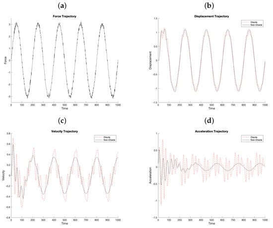
Figure 3. Force (a) Displacement (b), Velocity (c), and Acceleration (d) trajectories for Oracle and non-Oracle models with ${\sigma }_{ϵ}=0$.

3. Model Estimation

In an experimental setting, the data that will be observed at regular sampling times and contaminated with errors. For any time t the following likelihood is employed:

$${\overline{u}}_t,{\overline{v}}_t,{\overline{a}}_t|\theta ,\mathbf{f},\mathit{\epsilon }\sim \mathrm{MVN}\left[(u_t,v_t,a_t),\Sigma \right]$$

where $(u_t,v_t,a_t)$ is the solution of the differential equation at time t given the parameter values $\theta =\left(m,g,k_l,k_n,{\sigma }_{ϵ}^2,{\sigma }_u^2,{\sigma }_v^2,{\sigma }_a^2\right)$, forcing $\mathbf{f}$ and internal errors $\mathit{\epsilon }$; $\Sigma$ is a $3\times 3$ matrix with diagonal elements ${\sigma }_u^2,{\sigma }_v^2,{\sigma }_a^2$ and zeros elsewhere. It is assumed that the given the parameters and the resulting solution to the differential equations the residuals are independent across time. For notation, let $\overline{\mathbf{D}}=(\overline{\mathbf{u}},\overline{\mathbf{v}},\overline{\mathbf{a}})$ be the observed data.

A Bayesian approach is employed for inferences about the parameters and to create posterior predictive intervals. To obtain the posterior distribution of $\theta$ we use Bayes theorem given by (see [9]):

$$p(\theta ,\mathit{\epsilon }|\overline{\mathbf{D}},\mathbf{f})=\frac{L\left(\overline{\mathbf{D}}\right|\mathbf{f},\theta ,\mathit{\epsilon })p(\theta ,\mathit{\epsilon })}{\int L\left(\overline{\mathbf{D}}\right|\mathbf{f},\theta ,\mathit{\epsilon })p(\theta ,\mathit{\epsilon })d\theta }.$$

where:

$$L\left(\overline{\mathbf{D}}\right|\mathbf{f},\theta ,\mathit{\epsilon })=L(\overline{\mathbf{u}},\overline{\mathbf{v}},\overline{\mathbf{a}}|\mathbf{f},\theta ,\mathit{\epsilon })=\prod _{t=0}^{T}L({\overline{u}}_t,{\overline{v}}_t,{\overline{a}}_t|\mathbf{f},\theta ,\mathit{\epsilon }).$$

The following vague prior distributions are employed:

$$\begin{array}{ccc}\hfill {ϵ}_t|{\sigma }_{ϵ}^2& \sim & N(0,{\sigma }_{ϵ}^2),t=0,1,\dots ,T\hfill \\ \hfill {\sigma }_{ϵ}^2& \sim & \mathrm{Uniform}(0,Max{\sigma }_{ϵ}^2)\hfill \\ \hfill m& \sim & P(m=1)=1\hfill \\ \hfill g& \sim & N(0,100)\hfill \\ \hfill k_l& \sim & N(0,100)\hfill \\ \hfill k_n& \sim & N(0,100)\hfill \\ \hfill {\sigma }_u^2& \sim & {\chi }_2^2\hfill \\ \hfill {\sigma }_v^2& \sim & {\chi }_2^2\hfill \\ \hfill {\sigma }_a^2& \sim & {\chi }_2^2\hfill \end{array}$$

Using this prior distribution and likelihood specification the posterior distribution is not analytically tractable, hence sampling is employed. In this work, $Max{\sigma }_{ϵ}^2$ is set to 10 for ${\sigma }_{ϵ}^2$, which allows for high values (near 10) without the need to worry about extreme values as other distributions, such as an Inverse-Gamma, might provide. A Metropolis–Hastings embedded in a Gibbs sampler, where each parameter is sampled from its full conditional distribution using the Metropolis–Hastings algorithm, is implemented in MATLAB to obtain samples from the posterior distribution, with details given in Section 4. This algorithm was chosen as it is easy to implement in MATLAB.

3.1. Solving the Differential Equation

At each step of the Metropolis-Hastings sampler the differential equation needs to be solved regardless of whether the model is the Oracle or non-Oracle models. To solve the differential equation, the time interval $[0,T]$ is partitioned into N subintervals $[t^n,t^{n-1}]$, $n=1,\dots ,N$, with $t^0=0$ and $t^N=T$. For simplicity here, the time step $\Delta t$ is taken uniform. Given $u_0$ and $v_0$, the initial acceleration is estimated as:

$$a_0=\frac{1}{m}\left(f\left(0\right)-k{u}_0-\gamma v_0\right)$$

The acceleration, velocity, and displacement are updated at the subsequent time $t^n$, $n=1,\dots ,N$, as:

$$\begin{array}{cc}\hfill a_n& =\frac{f\left(t^n\right)-k{u}_{n-1}-(\gamma +\Delta t\lambda )v_{n-1}-[\gamma \Delta t(1-\lambda )+0.5k\Delta t^2(1-2\beta )]a_{n-1}}{m+\gamma \Delta t\lambda +k{\Delta }^2\beta }\hfill \end{array}$$

(14)

$$\begin{array}{cc}\hfill v_n& =v_{n-1}+\Delta t[\lambda a_n+(1-\lambda )a_{n-1}]\hfill \end{array}$$

(15)

$$\begin{array}{cc}\hfill u_n& =u_{n-1}+\Delta t{v}_{n-1}+0.5\Delta t^2{a}_{n-1}+\Delta t^2\beta (a_n-a_{n-1})\hfill \end{array}$$

(16)

where $\beta$ and $\lambda$ are the standard parameters of the Newmark scheme. The parameters are chosen here as $\beta =0.25$, $\gamma =0.5$, $\Delta t=0.1$, and $\lambda =0.5$. By choosing $\lambda =0.5$ and $\beta =0.25$ this represents the average constant acceleration scheme for the Newmark solver to ensures unconditional stability is achieved [10]. It should be noted that the settings for $\lambda$ and $\beta$ can influence the computational time for the solver. For example, $\lambda =0.5$ and $\beta =0.25$ the solver takes approximately 0.010 s to solve 1000 time steps, compared to when $\lambda =0.75$ and $\beta =0.25$ where the solver takes approximately 0.021 s to complete the computations; and when $\lambda =0.25$ and $\beta =0.25$, the solver takes approximately 0.018 s to complete the computations. Similarly, when $\lambda =0.5$ and $\beta =0.5$, the solver takes approximately 0.017 s to complete the same computations.

3.2. Verification Example

As a verification that the approach is viable, a dataset was generated using the sinusoidal forcing $\mathbf{f}$ given by Equation (9) with forcing parameters $A_c=5$, $n_c=5$, ${\sigma }_{ϵ}=0.5$, and model parameters $g=0.2$, $k_l=2.0$, $k_n=1.0$ and ${\sigma }_{ϵ}=0.5$. A total of 120,000 samples are taken from the posterior distribution using 10 chains of 12,000 with the first 2000 samples discarded as burn-in samples and the remaining 10,000 samples thinned by 10 resulting in 10 sets of 1000 samples resulting in 10,000 samples from which all inferences will be made. For the non-Oracle model the computing time is approximately 73.2 s and for the Oracle model the computing time is approximately 764.4 s. Sampler diagnostics, such as traceplots, as well as autocorrelation within chains, were examined for convergence, mixing, and to determine the thinning rate. Full computation details are presented in Section 4.

Table 1 shows the true values for the Oracle model and the 95% credible intervals based on sample quantiles, $(Q_{2.5},Q_{50},Q_{97.5})$, for both the Oracle and non-Oracle models. Notice that the posterior credible intervals correctly capture the true values of the model parameters. This provides evidence that the model parameter estimation approach is valid.

Table 1. Parameter estimates given by approximately 95% credible intervals, $(Q_{2.5},Q_{50},Q_{97.5})$, for both Oracle and non-Oracle models using simulated forcing data with $A_c=5$, ${\sigma }_{ϵ}=0.5$. Based on 10,000 posterior samples.

			${\mathit{A}}_{\mathit{c}}$
Model	$\theta$	True	$(Q_{2.5},Q_{50},Q_{97.5})$
Oracle	g	0.2	(0.145, 0.183, 0.267)
	$k_l$	2.0	(1.876, 2.065, 2.150)
	$k_n$	1.0	(0.896, 0.935, 1.088)
	${\sigma }_{ϵ}$	0.5	(0.469, 0.504, 0.545)
Non-Oracle	g	–	(0.247, 0.333, 0.415)
	$k_l$	–	(3.471, 3.526, 3.581)
	${\sigma }_{ϵ}$	–	(0.707, 0.787, 0.874)

4. Simulation Study

Of particular interest is model validation. Specifically, under what training dataset conditions are the models valid? Furthermore, under what conditions is the non-Oracle model competitive with the Oracle model? In this case, model validity is defined to be the predictive performance of the models for predicting both future values and maximum values. As this is a predictive study, a training dataset ${\overline{\mathbf{D}}}^{\mathcal{T}}=({\overline{\mathbf{u}}}^{\mathcal{T}},{\overline{\mathbf{v}}}^{\mathcal{T}},{\overline{\mathbf{a}}}^{\mathcal{T}})$ obtained using a training forcing ${\mathbf{f}}^{\mathcal{T}}$ is used to obtain samples from the posterior distribution of $\theta$. Additionally, a separate and independent validation forcing $\mathbf{f}$ is applied to obtain solutions $\mathbf{u},\mathbf{v},\mathbf{a}$. To validate the models the validation trajectories are compared with their posterior predictive distribution given by

$$p(\widehat{\mathbf{u}},\widehat{\mathbf{v}},\widehat{\mathbf{a}}|\overline{\mathbf{f}},{\mathbf{f}}^{\mathcal{T}},{\mathbf{D}}^{\mathcal{T}})=\int p(\widehat{\mathbf{u}},\widehat{\mathbf{v}},\widehat{\mathbf{a}}|\overline{\mathbf{f}},\theta ,\mathit{\epsilon })p\left(\mathit{\epsilon }\right|\theta )p\left(\theta \right|{\mathbf{f}}^{\mathcal{T}},{\mathbf{D}}^{\mathcal{T}})dϵd\theta .$$

To make the situation more realistic we accommodate possible internal errors in the system by using instead of the true forcing $\mathbf{f}$ a forcing contaminated by fixed realization of internal errors $\overline{\mathbf{f}}=\mathbf{f}-\mathit{\epsilon }$, where $\mathit{\epsilon }$ are independent centered Gaussian random variables with standard deviation ${\sigma }_e$. The training datasets are generated using Equation (9) with amplitude $A_c$ at the levels of 1 (low), 5 (medium), and 10 (high), and forcing error ${\sigma }_{ϵ}$ at $0.05$ (low), $0.5$ (medium), and $1.75$ (high). The model parameters are specified as $g=0.2$, $k_l=2.0$, $k_n=1.0$, and ${\sigma }_{ϵ}=0.5$ for all simulations. Since the interest is in estimating both future values and maximum value, the predictive distribution of the trajectories for all N time steps ahead are considered. Note that this is different from the traditional one, two, ten, etc., step ahead approach.

The validation forcings are generated using two regimes: Sinusoidal and Erratic. The Sinusoidal regime is uses Equation (9) with $A_c=5$ and centered Gaussian internal errors with ${\sigma }_{ϵ}=0.5$. Panel (a) of Figure 4 shows a representative realization of the Sinusoidal regime when the training dataset is generated using the same parameters. Furthermore, Figure 4 show the validation trajectories for displacement $\mathbf{u}$ (Panels b), velocity $\mathbf{v}$ (Panel c), and acceleration $\mathbf{a}$ (panel d) all with their 95% posterior predictive intervals. Notice that the posterior predictive intervals appear to have high coverage probabilities for displacement, velocity, and acceleration. This gives evidence that using sinusoidal training dataset gives a valid model for predicting the same system.

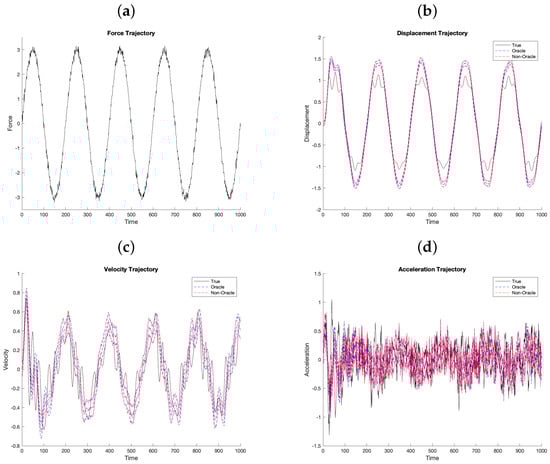
Figure 4. Training Force Contaminated with internal error (a) Displacement (b), Velocity (c) and Acceleration (d) trajectories. The Displacement, Velocity, and Accelerations have 95% posterior predictive intervals as well.

To understand how the sinusoidal training regime performs on a process that is dramatically different the Erratic regime is employed. The Erratic regime validation data generation processes is a realization of a sum of two stochastic processes. The first is a Gaussian moving average process with a small variance, ${\psi }_b^2$, serving as a background noise. The second process is a smoothed version of a marked Poisson process and models large shocks. The time of the large shocks is given by Poisson process with the amplitude modelled by a Gaussian random variable with a relatively large variance, ${\psi }_s^2$. Panel (a) of Figure 5 shows a representative realization. Notice that the process is very different from the sinusoidal process. However, by considering Panels (b, c, and d) one can see that the posterior predictive intervals appear to capture the process quite well.

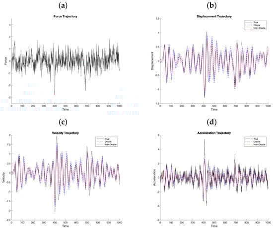
Figure 5. Validation Force (a) Displacement (b), Velocity (c), and Acceleration (d) trajectories. The Displacement, Velocity, and Accelerations have 95% posterior predictive intervals as well.

A simulation study is conducted by varying the training amplitude and assessing the performance of posterior predictive intervals on capturing the true value. The training datasets were created using the sinusoidal regime with amplitude, $A_c$ at levels 1, 5, and 10. These levels of $A_c$ are chosen so that there is a scenario in which a small, an accurate, and a large training amplitude is considered. The internal error standard deviation ${\sigma }_{ϵ}$ is also varied and set to levels $0.05$, $0.5$, and $1.75$ which correspond to a small, an accurate, and a large training noise. For each amplitude and noise combination 100 datasets were generated and MCMC samples from the posterior predictive distribution were obtained for each dataset for both the Oracle and non-Oracle models. For each amplitude, noise and Oracle/non-Oracle combination datasets two validation forcing datasets were generated, one using sinusoidal forcing and the other using erratic forcing. The simulation study was replicated 100 times. A Metropolis–Hastings embedded in a Gibbs sampler was implemented in MATLAB to obtain samples from the posterior predictive distribution. A total of 30,000 samples were taken from the posterior distribution with the first 20,000 samples discarded as burn-in samples and the remaining 10,000 samples thinned by 10 resulting in a set of 1000 samples from which all inferences will be made. Sampler diagnostics, such as traceplots, as well as autocorrelation within chains, were examined for convergence, mixing, and to determine the thinning rate. Example traceplots and auto-correlation plots for the Oracle model can be found in Figure A1 and Figure A2, respectively. Notice the chains appear to have converged and a thinning of every 10th sample will keep the auto-correlation between samples below 0.25. As one may be concerned with the choice of $Max{\sigma }_{ϵ}^2$ on its impact on the posterior distribution of ${\sigma }_{ϵ}^2$, a small sensitivity study is presented in Figure A3 that shows the kernel density estimates of the posterior distribution of ${\sigma }_{ϵ}^2$ when $Max{\sigma }_{ϵ}^2=0.5,1,2,5$, and 10. Notice that the posterior distributions in all cases essentially agree with each other, hence choice of $Max{\sigma }_{ϵ}^2=10$ should not have any large influence on the inferences.

Using the 2.5% and 97.5% quantiles from the MCMC samples from the posterior predictive distribution a 95% predictive interval is created for each ${\widehat{u}}_t$, ${\widehat{v}}_t$, and ${\widehat{a}}_t$ using each contaminated validation forcing $\overline{\mathbf{f}}$. Let $\mathbf{Z}$ be the solution attribute of interest, such as $\mathbf{u}$, $\mathbf{v}$ or $\mathbf{a}$ and $Z_{ti}$ be the true value of the attribute at time t for simulation replicate i and ${\widehat{\mathcal{Z}}}_{ti}$ be the 95% posterior predictive interval for the attribute at time t for simulation replicate i. The posterior predictive coverage rates for attribute Z were calculated using:

$$C\left(Z\right)=\frac{1}{100T}\sum _{i=1}^{100}\sum _{t=0}^{T}I\{Z_{ti}\in {\hat{\mathcal{Z}}}_{ti}\},$$

where $I\{Z_{ti}\in {\widehat{\mathcal{Z}}}_{ti}\}$ is an indicator function taking on the value 1 if $Z_{ti}\in {\widehat{\mathcal{Z}}}_{ti}$ and 0 otherwise.

Table 2 shows the results from the simulation study of the average coverage probability of the 95% posterior predictive intervals for $\widehat{\mathbf{u}}$, $\widehat{\mathbf{v}}$, and $\widehat{\mathbf{a}}$ for both Oracle and non-Oracle models across both validation regimes. Notice that for scenarios when ${\sigma }_{ϵ}$ is 0.5 or higher the coverage probabilities are quite good for all attributes, across all training amplitudes for both the Oracle and non-Oracle models using both Sinusoidal and Erratic validation forcing. Additionally, notice that the Oracle model performs reasonably well when ${\sigma }_{ϵ}$ is 0.05 when $A_c$ is 5 or 10. Furthermore, when the training Amplitude is higher the coverage probabilities are improve in all cases. This suggests that provided the typical range of the training forcing amplitude plus the internal error, $A_c+2{\sigma }_{ϵ}$, is larger than the typical forcing that would be applied in practice the non-Oracle model is valid for predicting the attributes. In cases where the typical forcing that would be applied in practice has low noise the Oracle model should be preferred.

Table 2. Average coverage probabilities of u, v, and a for both Oracle and non-Oracle models. The models were trained on a sinusoidal training system with amplitudes $A_c=1,3,5$, force error ${\sigma }_{ϵ}=0.05,0.5,1.75$ and validated on both Erratic and Sinusoidal systems with Erratic system with typical validation amplitude of 5, created using Erratic system variances ${\psi }_b^2=1,{\psi }_s^2=2.25$ and Sinusoidal parameters $A_p=5,{\sigma }_{ϵ}=0.5$. Based on 100 simulations.

			Sinusoidal			Erratic
			${\mathit{A}}_{\mathit{c}}$			${\mathit{A}}_{\mathit{c}}$
${\sigma }_{ϵ}$	Attribute	Oracle	1	5	10	1	5	10
0.05	u	Y	0.076	0.962	1.000	0.225	0.882	0.998
		N	0.243	0.215	0.197	0.221	0.189	0.178
	v	Y	0.113	0.962	1.000	0.211	0.927	0.998
		N	0.209	0.213	0.210	0.215	0.214	0.211
	a	Y	0.118	0.946	1.000	0.206	0.979	0.999
		N	0.204	0.216	0.239	0.213	0.235	0.261
0.5	u	Y	0.734	0.986	1.000	0.849	0.926	0.998
		N	0.929	0.989	0.988	0.989	0.969	0.972
	v	Y	0.910	0.987	1.000	0.849	0.963	0.999
		N	0.941	0.989	0.994	0.989	0.984	0.990
	a	Y	0.918	0.987	1.000	0.875	0.995	0.999
		N	0.946	0.991	0.997	0.991	0.994	0.998
1.75	u	Y	0.999	1.000	1.000	0.997	0.999	0.999
		N	0.990	1.000	1.000	0.995	1.000	0.999
	v	Y	1.000	1.000	1.000	0.996	0.999	1.000
		N	0.990	1.000	1.000	0.995	1.000	1.000
	a	Y	1.000	1.000	1.000	0.998	1.000	1.000
		N	0.990	1.000	1.000	0.995	1.000	1.000

Since the coverage probabilities are quite good when the training set exhibits more extreme amplitudes than the validation data one would like to determine the difference in the widths of the prediction intervals. Again, let Z be the solution attribute of interest, such as u, v or a, and $Z_{ti}$ be the true value of the attribute at time t for simulation replicate i and ${\widehat{\mathcal{Z}}}_{ti}$ be the 95% posterior predictive interval for the attribute at time t for simulation replicate i. The average posterior predictive interval widths, using an ${\mathcal{L}}_1$ norm, for attribute Z were calculated using:

$$W\left(Z\right)=\frac{1}{100T}\sum _{i=1}^{100}\sum _{t=0}^T\left|{\widehat{\mathcal{Z}}}_{ti}\right|.$$

Table 3 shows the average posterior predictive interval widths for u, v, and a for both Oracle and non-Oracle models using a training system with $A_c=1,3,5$ and internal error standard deviation ${\sigma }_{ϵ}=0.05,0.5,1.75$, and validated using both Erratic and Sinusoidal systems. Notice that the average interval widths are systematically higher for the non-Oracle versus the Oracle. This is to be expected since the non-Oracle model will always have a larger estimated internal error which is then propagated through the system. Furthermore, notice that the interval widths for the non-Oracle models are about twice the interval width of the Oracle models. Hence, the trade off of using the non-Oracle model is much wider predictive intervals.

Table 3. Average posterior predictive interval widths of u, v and a for both Oracle and non-Oracle models. The models were trained on a sinusoidal training system with amplitudes $A_c=1,3,5$, force error ${\sigma }_{ϵ}^2=0.05,0.5,1.75$ and validated on both Erratic and Sinusoidal systems with Erratic system with typical validation amplitude of 5, created using Erratic system variances ${\psi }_b^2=1,{\psi }_s^2=2.25$ and Sinusoidal parameters $A_p=5,{\sigma }_{ϵ}=0.5$. Based on 100 simulations.

			Sinusoidal			Erratic
			${\mathit{A}}_{\mathit{c}}$			${\mathit{A}}_{\mathit{c}}$
${\sigma }_{ϵ}$	Attribute	Oracle	1	5	10	1	5	10
0.05	u	Y	0.151	0.139	0.140	0.125	0.090	0.090
		N	0.193	0.259	0.435	0.601	0.204	0.344
	v	Y	0.230	0.211	0.212	0.268	0.199	0.200
		N	0.291	0.401	0.854	0.434	0.395	0.348
	a	Y	0.542	0.517	0.520	0.741	0.613	0.613
		N	0.621	0.757	1.833	0.963	0.955	0.848
0.5	u	Y	0.309	0.152	0.135	0.292	0.096	0.090
		N	0.631	0.264	0.430	0.616	0.204	0.344
	v	Y	0.472	0.231	0.205	0.454	0.211	0.199
		N	0.951	0.411	0.843	0.586	0.394	0.360
	a	Y	0.820	0.540	0.513	1.136	0.635	0.612
		N	1.533	0.770	1.811	1.132	0.954	0.875
1.75	u	Y	0.294	0.276	0.232	0.477	0.243	0.151
		N	1.314	0.360	0.375	0.715	0.226	0.356
	v	Y	0.512	0.436	0.361	0.488	0.343	0.278
		N	2.178	0.622	0.696	1.139	0.408	0.384
	a	Y	0.840	0.809	0.711	1.706	0.958	0.770
		N	3.677	1.206	1.465	2.049	0.977	0.931

The results from the simulation study above show that both the Oracle and non-Oracle models perform well when considering estimating the true value of the system. Since mechanical systems often fail at the extremes engineers are quite interested in predicting the extreme values of the system across time. To study this a simulation study was conducted using the same simulation experimental design, MCMC sampling scheme, and replications as above with the maximum values of each of the attributes as the quantity of interest. As above, let Z denote the attribute of interest, typically displacement, velocity, or acceleration. To obtain a posterior predictive interval for $M=max\left\{Z\right\}$ the following approach is used. For the $m^{th}$ draw from the posterior distribution of $\theta$, the corresponding solution trajectory for Z is created without using external error. The solution is denoted by ${\tilde{Z}}_t^{\left(m\right)}$ for times $t=0,1,...T$, and the maximum value across t is obtained, ${\tilde{M}}^{\left(m\right)}=max\{{\tilde{Z}}_t^{\left(m\right)}:0,1,...,T\}$. Finally, the external error with variance given by the corresponding mth posterior sample is added to obtain ${\left\{{\widehat{M}}^{\left(m\right)}\right\}}_{m=1}^{1000}$. The 2.5% and 97.5% quantiles for ${\left\{{\widehat{M}}^{\left(m\right)}\right\}}_{m=1}^{1000}$ are used to create a 95% posterior predictive interval for M denoted by $\widehat{\mathcal{M}}$. Let $M_i$ be the true maximum value of the system under forcing ${\mathbf{f}}_i$ for simulation replicate i and ${\widehat{\mathcal{M}}}_i$ be the corresponding 95% posterior predictive interval of the maximum value. The coverage posterior predictive coverage rates for the maximum were calculated using:

$$C\left(M\right)=\frac{1}{100}\sum _{i=1}^{100}I\{M_i\in {\widehat{\mathcal{M}}}_i\},$$

where $I\{M_i\in {\widehat{\mathcal{M}}}_i\}$ is an indicator function taking on the value 1 if $Z_{ti}\in {\widehat{\mathcal{Z}}}_{ti}$ and 0 otherwise.

Table 4 shows the results of the coverage probabilities when using the posterior predictive distribution to predict the maximum value for each attribute for both Oracle and non-Oracle models across various Sinusoidal training amplitudes and noise for both Sinusoidal and Erratic validation regimes. Notice that the results are much different when attempting to predict the maximum value. Both the Oracle and non-Oracle methods work well when the validation forcing has similar amplitude and error as the training amplitude and errors. Consider when ${\sigma }_{ϵ}=0.5$ and $A_c=5$ then coverage probabilities for the maximum value are high across both Sinusoidal and Erratic validation regimes and across all attributes. When ${\sigma }_{ϵ}=0.05$ and $A_c=5$ then the Oracle model appears to work well but the non-Oracle model does not. This is consistent across all attributes and both validation regimes. When ${\sigma }_{ϵ}$ is large relative to the training error and when the training and validation amplitudes differ both the Oracle and non-Oracle models perform poorly across both validation regimes.

Table 4. Coverage probabilities of maximum values for u, v, and a for both Oracle and non-Oracle models. The models were trained on a sinusoidal training system with amplitudes $A_c=1,3,5$, force error ${\sigma }_{ϵ}=0.05,0.5,1.75$ and validated on both Erratic and Sinusoidal systems with Erratic system with typical validation amplitude of 5, created using Erratic system variances ${\psi }_b^2=1,{\psi }_s^2=2.25$ and Sinusoidal parameters $A_p=5,{\sigma }_{ϵ}=0.5$. Based on 100 simulations.

			Sinusoidal			Erratic
			${\mathit{A}}_{\mathit{c}}$			${\mathit{A}}_{\mathit{c}}$
${\sigma }_{ϵ}$	Attribute	Oracle	1	5	10	1	5	10
0.05	u	Y	0.00	1.00	0.85	0.25	0.93	0.39
		N	0.24	0.12	0.10	0.31	0.15	0.13
	v	Y	0.18	0.99	0.00	0.31	0.99	0.06
		N	0.09	0.09	0.19	0.17	0.17	0.23
	a	Y	0.00	0.83	0.00	0.03	0.97	0.02
		N	0.01	0.00	0.00	0.11	0.05	0.09
0.5	u	Y	0.00	1.00	0.64	0.31	0.96	0.24
		N	0.41	1.00	1.00	0.40	1.00	0.99
	v	Y	0.66	1.00	0.01	0.33	1.00	0.03
		N	0.58	1.00	1.00	0.42	0.99	0.99
	a	Y	0.98	1.00	0.00	0.63	0.98	0.01
		N	0.61	1.00	1.00	0.60	0.99	1.00
1.75	u	Y	0.00	0.58	0.31	0.01	0.61	0.33
		N	0.07	0.71	0.98	0.07	0.48	0.86
	v	Y	0.00	0.58	0.14	0.01	0.56	0.21
		N	0.01	0.32	0.93	0.04	0.39	0.89
	a	Y	0.00	0.50	0.03	0.00	0.35	0.06
		N	0.00	0.10	0.74	0.04	0.22	0.85

5. Discussion

This work introduced a novel approach to both quantify the uncertainty associate with model misspecification, as well as create predictive distributions that incorporate this uncertainty. By introducing an “inside” error term, $ϵ$ into the system captures the model misspecification and forcing noise which is quantified in the ${\sigma }_{ϵ}$ parameter. A Bayesian approach allows for the estimation of the model parameters, as well as the posterior predictive distributions. The posterior distribution of ${\sigma }_{ϵ}$ allows for the study of the misspecification uncertainty where large values of ${\sigma }_{ϵ}$ would indicate a large model misspecification and small values would indicate the model is reasonably specified. Furthermore, by propagating the error associated with model misspecification the misspecified model can be can be made into a valid predictive model for estimating the mean value of the system. In certain conditions, one can also achieve this for estimating the maximum value of the system. However, care should be taken in both of these cases to ensure that the training dataset is representative of conditions that the real system may experience.

The single degree of freedom oscillator is used as a simple example to illustrate the method. Extending this approach into systems such as Elasto-Plastic model, Accelerometer, Seismometer, and Estimates of Peak Roof Displacement [6,11]. Other applications include dynamic behavior of systems with fractional damping and dynamical analysis on single degree of freedom semi-active control systems with a fractional order derivative [12,13]. Another extension of this work could be to model space-time phenomena similar to those studied by [14], as there is inherent error in the model structure, as well as measurement error. One important question that needs consideration is the structure of the internal and external errors and their impact on resulting inferences. In the case that the Gaussian likelihood assumption is not valid, one may need to consider other estimation procedures than Metropolis-Hastings samplers and may wish to consider Approximate Bayesian Computation (ABC). For a good overview of using ABC with dynamical models, see [15].

The approach presented is computationally intensive which may be prohibitive for complex systems that in and of themselves are computationally demanding. Nevertheless, as computation speed and capacity increases this approach may become viable for more and more complex models.

Appendix A.1

This section shows the MCMC diagnostics used for the samples obtained via the Metropolis–Hastings sampler. The Oracle model was considered with $g=0.2$, $k_l=2$, $k_n=1$, $si{g}_{ϵ}=0.5$, $si{g}_u=1$, and $si{g}_v=1$. Figure A1 shows the trace plots for the 10,000 MCMC samples for g (panel a), $k_l$ (panel b), $k_n$ (panel c), ${\sigma }_{ϵ}$ (panel d), ${\sigma }_u$ (panel e), and ${\sigma }_v$ (panel f). Notice that the sampler appears to have converged for each of the parameters as all traceplots are near stationary.

Figure A1. Exampletraceplots from the MCMC samples g (panel a), $k_l$ (panel b), $k_n$ (panel c), ${\sigma }_{ϵ}$ (panel d), ${\sigma }_u$ (panel e), and ${\sigma }_v$ (panel f).

Figure A2 shows the auto-correlation plots for the pre-thinned 100,000 MCMC samples for g (panel a), $k_l$ (panel b), $k_n$ (panel c), ${\sigma }_c$ (panel d), ${\sigma }_u$ (panel e), and ${\sigma }_v$ (panel f). Thinning by every 10th sample will keep the auto-correlation between sequential samples below 0.25.

Figure A2. Example autocorrelation plots from the MCMC samples: g (panel a), $k_l$ (panel b), $k_n$ (panel c), ${\sigma }_{ϵ}$ (panel d), ${\sigma }_u$ (panel e), and ${\sigma }_v$ (panel f).

Appendix A.2

Figure A3 shows the kernel density estimates for ${\sigma }_{ϵ}^2$ for prior specifications of ${\sigma }_{ϵ}^2\sim Uniform(0,Max{\sigma }_{ϵ}^2)$ where $Max{\sigma }_{ϵ}^2=0.5,1,2,5$, and 10. Notice that the posterior density estimates agree with each other quite well across all values of $Max{\sigma }_{ϵ}^2$, suggesting that the influence of $Max{\sigma }_{ϵ}^2$ is minimal on inferences.

Figure A3. Kernel density estimates of the posterior distribution for ${\sigma }_{ϵ}^2$ across prior distribution parameter specifications of $Max{\sigma }_{ϵ}^2=0.5,1,2,5$, and 10.

References

- Kennedy, M.C.; O’Hagan, A. Bayesian Calibration of Computer Models. J. R. Stat. Soc. B 2001, 63, 425–464. [Google Scholar] [CrossRef]
- Chkrebtii, O.A.; Campbell, D.A.; Calderhead, B.; Girolami, M.A. Bayesian Solution Uncertainty Quantification for Differential Equations. Bayesian Anal. 2016, 11, 1239–1267. [Google Scholar] [CrossRef]
- Morrison, R.E.; Oliver, T.A.; Moser, R.D. Representing model inadequacy: A stochastic operator approach. SIAM/ASA J. Uncertain. Quantif. 2018, 6, 457–496. [Google Scholar] [CrossRef]
- Wu, S.; Hannig, J.; Lee, C.M.T. Uncertainty quantification for principal component regression. Electron. J. Stat. 2021, 15, 2157–2178. [Google Scholar] [CrossRef]
- Lee, S.H.; Chen, W. A comparative study of uncertainty propagation methods for black-box-type problems. Struct. Multidiscip. Optim. 2009, 37, 239–253. [Google Scholar] [CrossRef]
- Strong, M.; Oakley, J.E. When Is a Model Good Enough? Deriving the Expected Value of Model Improvement via Specifying Internal Model Discrepancies. J. Uncertain. Quantif. 2014, 2, 106–125. [Google Scholar] [CrossRef]
- Gelman, A.; Carlin, J.B.; Stern, H.S.; Dunson, D.B.; Vehtari, A.; Rubin, D.B. Bayesian Data Analysis, 3rd ed.; CRC Press: Boca Raton, FL, USA, 2013. [Google Scholar]
- Liu, F.; Bayarri, M.J.; Berger, J.O. Modularization in Bayesian Analysis, with Emphasis on Analysis of Computer Models. Bayesian Anal. 2009, 4, 119–150. [Google Scholar] [CrossRef]
- Berger, J.O. Statistical Decision Theory and Bayesian Analysis, 2nd ed.; Springer: New York, NY, USA, 1985. [Google Scholar]
- Newmark, N.M. A method of computation for structural dynamics. J. Eng. Mech. Div. 1959, 85, 67–94. [Google Scholar] [CrossRef]
- Newman, J.; Makarenkov, P. Resonance oscillations in a mass-spring impact oscillator. Nonlinear Dyn. 2015, 79, 111–118. [Google Scholar] [CrossRef]
- Shen, Y.; Fan, M.; Li, X.; Yang, S.; Xing, H. Dynamical Analysis on Single Degree-of-Freedom Semiactive Control System by Using Fractional-Order Derivative. Math. Probl. Eng. 2015, 2015, 272790. [Google Scholar] [CrossRef]
- Zarraga, O.; Sarría, I.; Garcxixa-Barruetabeña, J.; Cortés, F. An Analysis of the Dynamical Behaviour of Systems with Fractional Damping for Mechanical Engineering Applications. Symmetry 2019, 11, 1499. [Google Scholar] [CrossRef]
- Wikle, C.K.; Berliner, L.M.; Cressie, N. Hierarchical Bayesian space-time models. Environ. Ecological Stat. 1998, 5, 117–154. [Google Scholar] [CrossRef]
- Toni, T.; Welch, D.; Strelkowa, N.; Ipsen, A.; Stumpf, M.P.H. Approximate Bayesian computation scheme for parameter inference and model selection in dynamical systems. J. R. Soc. Interface 2009, 6, 187–202. [Google Scholar] [CrossRef] [PubMed]
Publisher’s Note: MDPI stays neutral with regard to jurisdictional claims in published maps and institutional affiliations. |
© 2022 by the authors. Licensee MDPI, Basel, Switzerland. This article is an open access article distributed under the terms and conditions of the Creative Commons Attribution (CC BY) license (https://creativecommons.org/licenses/by/4.0/).