On Synthetic Interval Data with Predetermined Subject Partitioning and Partial Control of the Variables’ Marginal Correlation Structure

Abstract

A standard approach for assessing the performance of partition models is to create synthetic datasets with a prespecified clustering structure and assess how well the model reveals this structure. A common format involves subjects being assigned to different clusters, with observations simulated so that subjects within the same cluster have similar profiles, allowing for some variability. In this manuscript, we consider observations from interval variables. Interval data are commonly observed in cohort and Genome-Wide Association studies, and our focus is on Single-Nucleotide Polymorphisms. Theoretical and empirical results are utilized to explore the dependence structure between the variables in relation to the clustering structure for the subjects. A novel algorithm is proposed that allows control over the marginal stratified correlation structure of the variables, specifying exact correlation values within groups of variables. Practical examples are shown, and a synthetic dataset is compared to a real one, to demonstrate similarities and differences.

1. Introduction

Partitioning and mixture models are often used to reveal the clustering structure within a sample, for example, to discover if combinations of risk factors are associated with the risk of disease [1], or to reveal dependencies in a population after reducing the dimensionality of the problem [2]. An overview of clustering approaches is given in [3,4]. Sometimes, partitioning the variables rather than the subjects is of interest [5,6]. In this manuscript, we focus on the more standard set-up where subjects are partitioned, but the two frameworks can be viewed as interchangeable for simulated observations.

We adopt a model-based approach, and define as a cluster each one of the components of the adopted mixture model. Therefore, we undertake that two subjects belong to the same cluster when the corresponding vectors of observations are generated by the same component of the mixture model. See [7] for an extensive discussion on cluster definition. Assessing the performance of partitioning models involves the creation of synthetic data with a prespecified clustering structure. The model is then fitted to the simulated data to evaluate its performance in terms of revealing this structure.

For continuous observations, partitioning models often allow for a specific correlation structure for the variables, given the cluster allocation [8]. This typically involves a multivariate normal distribution [9]. Clustering approaches for observations from interval variables often prescribe that variables are independent, given the clustering of the subjects [10,11]. The resulting dimensionality reduction is the main advantage of this local independence modeling, as determining a fully specified joint distribution between P variables with M levels requires the specification of $M^P$ probabilities, a task that quickly becomes cumbersome and unwieldy. The authors of [12] comment on this notable modeling difference, mentioning that, in many applications, conditional independence has proven successful in achieving the main objective of a clustering algorithm, which is to bring together similar observations. In [13], local dependence is discussed, given well-defined substantive interest.

In this manuscript, we adopt the widely espoused independence assumption for the variables conditionally on the clustering of the subjects. In all examples, we ensure that clustering structures are identifiable, up to label switching, by following the guidelines of [14] for the required number of variables for mixture models when the within-cluster independence assumption holds. Thus, with C denoting the number of clusters, all synthetic datasets satisfy the identifiability condition $P\ge 2[{log}_M\left(C\right)]+1$.

Our work concerns interval variables, where the numerical distance between possible values is meaningful and known. Interval variables are of particular interest to us, as data from epidemiological and association cohort studies, such as the number of genetic variants, are often in this form. Furthermore, continuous observations are often transformed to interval ones when data from cohort studies are analyzed. This is performed to alleviate the adverse effect of outlier observations (for example, in dietary observations; see [15]), or to allow for the flexible modeling of interactions. Importantly, interval variables allow for the use of covariances and correlations through expectations. The variables are assumed to be independent given the clustering of the subjects, but they can be marginally dependent, i.e., dependent after the cluster allocation variables are summed out. In synthetic datasets, the induced marginal dependence is typically ignored and can be at odds with the dependence structure observed in real datasets.

The aim of this manuscript is to provide theoretical and computational tools for the creation of simulated datasets relevant to clustering algorithms, so that the synthetic data share more characteristics with real ones compared to synthetic data created with standard methods. An algorithm is proposed where the clustering structure is predetermined, while maintaining partial control over the marginal dependence structure between the variables. To the best of our knowledge, no such algorithm has yet been proposed. Our focus is on generating simulated datasets that contain observations that emulate Single-Nucleotide Polymorphisms (SNPs), although the proposed methods are more generally applicable. We do not touch on issues relevant to recombination and imputation [16], as these are beyond the scope of this manuscript.

Approaches in the literature relevant to marginal correlations focus on continuous observations, and on deriving association measures that provide unbiased estimates of marginal correlations when the size of the cluster relates to some outcome and a random effects-type model is utilized [17,18]. Consequently, the relevance of these approaches to the work presented in this manuscript is limited. Ref. [19] discusses the simulation of correlated binary observations, incorporating cluster-specific random effects, but the aim of the algorithm is not to generate clusters with distinct variable profiles.

In Section 2, we describe the generic approach for creating data with a predetermined clustering structure, and explore the marginal dependence structure between interval variables, deriving theoretical results. Based on Proposition 1, we propose the main algorithm of the manuscript in Section 3. Proposition 2 in the same section proves that the algorithm creates a stratified marginal correlation structure between the variables, where any two variables within the same stratum have the same correlation. Proposition 3, still in Section 3, provides the theoretical result that allows the user to control the magnitude of the covariances or correlations between variables that belong to the same stratum. In Section 4, a synthetic dataset is created using the proposed algorithm, and is compared to a real dataset that contains SNP observations, demonstrating similarities and differences between the two dependence structures. We conclude with a discussion in Section 5.

2. Materials and Methods

2.1. The Clustering Model

Assume P variables $x_{.p}$, $p=1,\dots ,P$. Without any loss of generality, assume that each variable takes values $1,\dots ,M_p$. Let $x=(x_{.1},\dots ,x_{.P})$. Denote by n the number of subjects. For subject i, $i=1,\dots ,n$, and a variable profile $x_i$ is a set of values $x_i=\{x_{i1},\dots ,x_{iP}\}$. Let $z=(z_1,\dots ,z_n)$, where $z_i$ is an allocation variable, so that $z_i=c$ denotes that subject i belongs to cluster c. Denote by ${\varphi }_p^c\left(x\right)$ the probability that $x_{.p}=x$ when the individual belongs to cluster c. Given the clustering allocation, the variables are assumed to be independent, each one following a multinomial distribution with cluster-specific parameters ${\mathit{\varphi }}_p^c=({\varphi }_p^c\left(1\right),\dots ,{\varphi }_p^c\left(M_p\right))$. Denote by $\mathit{\psi }=\{{\psi }_1,{\psi }_2,\dots ,{\psi }_C\}$ the probabilities that a subject belongs to cluster c, $c=1,\dots ,C$. For more on finite Bayesian mixture models, see [20].

2.2. A Generic Algorithm for a Predetermined Clustering Structure

A generic algorithm for creating observations from P variables, for subjects that are partitioned in C clusters, can be obtained via the following steps:

• Specify the number of clusters C.
• Specify the number of subjects $n_c$, where $c=1,\dots ,C$ is allocated to cluster c in accordance with cluster allocation probabilities ${\psi }_c$. Allocate subjects to clusters so that exactly $n_c$ subjects are allocated to cluster c. [Alternatively, a cluster can be drawn for a subject according to the allocation probabilities.]
• Specify the variable profile of the subjects within each cluster, i.e., probabilities $P(x_{.p}=x_{ip}|z_i=c)={\varphi }_p^c\left(x_{ip}\right)$, for all $c=1,\dots ,C$, $p=1,\dots ,P$, and $x_{ip}=1,\dots ,M_p$, to generate a distinct variable profile for the subjects in each cluster.
• To generate $x_{ip}$, sample from a multinomial distribution with probabilities ${\mathit{\varphi }}_p^{z_i}$.

2.3. The Marginal Correlation Structure of Interval Variables

Assume that x is a vector of interval variables. The marginal variance–covariance matrix is as follows:

$$\begin{gathered} \mathrm{Var}\left(\mathit{x}\right)=\mathrm{E}\left(\mathit{x}{\mathit{x}}^{\top }\right)-\mathrm{E}\left(\mathit{x}\right)\mathrm{E}{\left(\mathit{x}\right)}^{\top } \\ ={\mathrm{E}}_{\mathit{z}}{\mathrm{E}}_{\mathit{x}|\mathit{z}}\left(\mathit{x}{\mathit{x}}^{\top }\right|\mathit{z})-\left({\mathrm{E}}_{\mathit{z}}{\mathrm{E}}_{\mathit{x}|\mathit{z}}\left(\mathit{x}\right|\mathit{z})\right)\left({\mathrm{E}}_{\mathit{z}}{\mathrm{E}}_{\mathit{x}|\mathit{z}}{\left(\mathit{x}\right|\mathit{z})}^{\top }\right). \end{gathered}$$

Element $(p,p)$, $p=1,\dots ,P$ in the diagonal of $\mathrm{Var}\left(x\right)$ is as follows:

$$\begin{array}{ccc}\hfill \mathrm{Var}\left(x_{.p}\right)& =& \mathrm{E}\left(x_{.p}^2\right)-\mathrm{E}{\left(x_{.p}\right)}^2\hfill \\ & =& \sum _{x_p=1}^{M_p}{x}_p^{2}P(x_{.p}=x_p)-{[\sum _{x_p=1}^{M_p}{x}_{p}P(x_{.p}=x_p)]}^2\hfill \end{array}$$

After introducing the cluster allocation variables through the Law of Total Probability,

$$\begin{array}{ccc}\hfill \mathrm{Var}\left(x_{.p}\right)& =& \sum _{c=1}^C{\psi }_c[\sum _{x_p=1}^{M_p}{x}_p^{2}P(x_{.p}=x_p|z_i=c)]\hfill \\ & & -{\{\sum _{c=1}^C{\psi }_c[\sum _{x_p=1}^{M_p}{x}_{p}P(x_{.p}=x_p|z_i=c)]\}}^2.\hfill \end{array}$$

(1)

Element $(p,q)$, $p\ne q$, $p,q=1,\dots ,P$ in the off-diagonal of $\mathrm{Var}\left(x\right)$ is as follows:

$$\begin{array}{ccc}\hfill \mathrm{Cov}(x_{.p},x_{.q})& =& \mathrm{E}(x_{.p}\times x_{.q})-\mathrm{E}(x_{.p})\times \mathrm{E}(x_{.q})\hfill \\ & =& \sum _{x_p=1}^{M_p}\sum _{x_q=1}^{M_q}{x}_p\times x_{q}P(x_{.p}=x_p,x_{.q}=x_q)\hfill \\ & & -\sum _{x_p=1}^{M_p}{x}_{p}P(x_{.p}=x_p)\times \sum _{x_q=1}^{M_q}{x}_{q}P(x_{.q}=x_q)\hfill \\ & =& \{\sum _{c=1}^{C}P(z_i=c)\sum _{x_p=1}^{M_p}\sum _{x_q=1}^{M_q}{x}_p{x}_{q}P(x_{.p}=x_p,x_{.q}=x_q|z_i=c)\}\hfill \\ & & -\{\sum _{c=1}^{C}P(z_i=c)[\sum _{x_p=1}^{M_p}{x}_{p}P(x_{.p}=x_p|z_i=c)]\}\hfill \\ & & \times \{\sum _{c=1}^{C}P(z_i=c)[\sum _{x_q=1}^{M_q}{x}_{q}P(x_{.q}=x_q|z_i=c)]\}.\hfill \end{array}$$

As $x_{.p}$ and $x_{.q}$ are independent given z,

$$\begin{array}{ccc}\hfill \mathrm{Cov}(x_{.p},x_{.q})& =& \sum _{c=1}^{C}P(z_i=c)[\sum _{x_p=1}^{M_p}{x}_{p}P(x_{.p}=x_p|z_i=c)][\sum _{x_q=1}^{M_q}{x}_{q}P(x_{.q}=x_q|z_i=c)]\hfill \\ & & -\{\sum _{c=1}^{C}P(z_i=c)[\sum _{x_p=1}^{M_p}{x}_{p}P(x_{.p}=x_p|z_i=c)]\}\hfill \\ & & \times \{\sum _{c=1}^{C}P(z_i=c)[\sum _{x_q=1}^{M_q}{x}_{q}P(x_{.q}=x_q|z_i=c)]\}\hfill \\ & =& \sum _{c=1}^C{\psi }_c[\sum _{x_p=1}^{M_p}{x}_{p}P(x_{.p}=x_p|z_i=c)][\sum _{x_q=1}^{M_q}{x}_{q}P(x_{.q}=x_q|z_i=c)]\hfill \\ & & -\{\sum _{c=1}^C{\psi }_c[\sum _{x_p=1}^{M_p}{x}_{p}P(x_{.p}=x_p|z_i=c)]\}\hfill \\ & & \times \{\sum _{c=1}^C{\psi }_c[\sum _{x_q=1}^{M_q}{x}_{q}P(x_{.q}=x_q|z_i=c)]\}.\hfill \end{array}$$

Denote by $f_{p,c}$ the expected value for $x_{.p}$ in cluster c, i.e., $f_{p,c}=\mathrm{E}\left(x_{.p}\right|z_i=c)={\sum }_{x_p=1}^{M_p}{x}_{p}P(x_{.p}=x_p|z_i=c)$. Then, for $p\ne q$,

$$\begin{array}{cc}& \mathrm{Cov}(x_{.p},x_{.q})={\sum }_{c=1}^C{\psi }_c{f}_{p,c}{f}_{q,c}-\left({\sum }_{c=1}^C{\psi }_c{f}_{p,c}\right)\left({\sum }_{c=1}^C{\psi }_c{f}_{q,c}\right).\end{array}$$

(2)

Example 1.

Consider $C=4$, and assume that $f_{p,1}=f_{q,1}=f_{p,3}=f_{q,3}$ and $f_{p,2}=f_{q,2}=f_{p,4}=f_{q,4}$. Then, for $p\ne q$, it follows from (2) that

$$Cov(x_{.p},x_{.q})=({\psi }_1+{\psi }_3)({\psi }_2+{\psi }_4){(f_{p,1}-f_{p,2})}^2>0.$$

In the Supplementary Material, Section S2, we present an extended version of Example 1, as well as an additional example of inferences after utilizing Equation (2). However, the larger the number of clusters, the less helpful (2) becomes for understanding the effect of the clustering on the marginal covariance structure of the variables. More helpful is the following proposition:

Proposition 1.

Assume that $x_{.p}$ and $x_{.q}$ are interval variables. Under the condition that ${\psi }_1={\psi }_2=\dots ={\psi }_C=\psi$, for $p\ne q$, $p,q=1,\dots ,P$,

$$\begin{array}{ccc}& & Cov(x_{.p},x_{.q})=\sum _{\{c_1,c_2=1,\dots ,C,c_1<c_2\}}{\psi }^2(f_{p,c_1}-f_{p,c_2})(f_{q,c_1}-f_{q,c_2}).\hfill \end{array}$$

(3)

Proof. 

The proof is given in the Appendix A. □

Equation (3), although restricted to ${\psi }_c=\psi$, $c=1,\dots ,C$, is more helpful for examining the effect of the clustering on the marginal covariance structure of the variables. For any number of clusters, if, for all $c_1<c_2$, the sign of $(f_{p,c_1}-f_{p,c_2})$ is the same as the sign of $(f_{q,c_1}-f_{q,c_2})$, the correlation between $x_{.p}$ and $x_{.q}$ is positive. If, for all $c_1<c_2$, the sign of $(f_{p,c_1}-f_{p,c_2})$ is different to the sign of $(f_{q,c_1}-f_{q,c_2})$, the correlation between $x_{.p}$ and $x_{.q}$ is negative. The correlation is zero if, for every term in $\mathrm{Cov}(x_{.p},x_{.q})$, as given by (3), either $f_{p,c_1}=f_{p,c_2}$ or $f_{q,c_1}=f_{q,c_2}$.

The R code for theoretically evaluating correlation structures, for simulating datasets under the different scenarios and specifications relevant to our manuscript, and for replicating the analyses shown in the main manuscript and the Supplementary Material is available to download.

3. Results

3.1. An Algorithm for a Predetermined Subject Clustering with Partial Control of the Variables’ Dependence Structure

Let $H_p$, $p=1,\dots ,P$ denote a probability vector that contains $M_p$ probabilities that add up to 1. Let also $L_p$, $p=1,\dots ,P$ denote a different probability vector that contains $M_p$ probabilities that add up to 1. According to the algorithm proposed in this section, markedly different vectors, $H_p$ and $L_p$, will create distinct profiles for subjects in different clusters. The algorithm generates $k=2^{C/2-1}$ strata or groups of variables, where the dependence between variables (as specified by the correlation) within a group is stronger compared to the dependence between variables in different groups. This equation allows the user to define either the number of clusters for the subjects or the number of groups of variables, with the other quantity specified accordingly. Henceforth, we refer to those groups of variables as omogenous, as the correlation between any two variables within the same group is the same.

The derived dependence structure is shown empirically in Example 2, where we present sample correlations assuming interval variables. The algorithm allows for homogenous groups of different sizes. In Section 3.2, we derive a theoretical result for interval variables that allows prespecification of within-group covariances or correlations. In turn, this specification determines what $H_p$ and $L_p$ should be. We determine C to be even, as this generates a clearly defined dependence structure. This is shown in Examples S3 and S4 in Section S3 of the Supplementary Material, where a variation of the proposed algorithm is considered that allows for an odd C. The variables are positively correlated within each homogenous group of variables.

The proposed algorithm is shown below. Explanatory comments are added in brackets.

(1)

Define the number k of homogenous groups of variables, where k is a power of 2.

{Solving $k=2^{C/2-1}$ provides the even number of clusters, $C=2\ast [ln(k)/ln(2)+1]$.}

(2)

Define the number of variables $l_v$ in each homogenous group v, $v=1,\dots ,k$.

(3)

Define the number of subjects, $n_1=\dots =n_C$, within each cluster.

(4)

For each variable $x_{.p}$, consider two sets of probabilities,

$H_p=\{{\varphi }_p^H\left(1\right),\dots ,{\varphi }_p^H\left(M_p\right)\}$ and $L_p=\{{\varphi }_p^L\left(1\right),\dots ,{\varphi }_p^L\left(M_p\right)\}$, so that

${\sum }_{m=1}^{M_p}{\varphi }_p^H\left(m\right)=1$ and ${\sum }_{m=1}^{M_p}{\varphi }_p^L\left(m\right)=1$.

The two sets could be distinct so that the first elements of $H_p$ are considerably higher than subsequent elements, whilst the first elements of $L_p$ are considerably lower.

(5)

For an odd c, define the profile of cluster c so that the following apply:

–

The first $l_1+\dots +l_{k/\left(2^{c/2-0.5}\right)}$ variables are simulated in accordance with $\{L_1,\dots ,L_P\}$;

–

The next $l_{k/\left(2^{c/2-0.5}\right)+1}+\dots +l_{k/\left(2^{c/2-0.5}\right)+k/\left(2^{c/2-0.5}\right)}$ variables are simulated in accordance with $\{H_1,\dots ,H_P\}$;

–

The next $l_{k/\left(2^{c/2-0.5}\right)+k/\left(2^{c/2-0.5}\right)+1}+\dots +l_{k/\left(2^{c/2-0.5}\right)+k/\left(2^{c/2-0.5}\right)+k/\left(2^{c/2-0.5}\right)}$ variables are simulated in accordance with $\{L_1,\dots ,L_P\}$;

–

And so on and so forth.

(6)

For an even c, define the profile of cluster c so that the following apply:

–

The first $l_1+\dots +l_{k/\left(2^{c/2-1}\right)}$ variables are simulated in accordance with $\{H_1,\dots ,H_P\}$;

–

The next $l_{k/\left(2^{c/2-1}\right)+1}+\dots +l_{k/\left(2^{c/2-1}\right)+k/\left(2^{c/2-1}\right)}$ variables are simulated in accordance with $\{L_1,\dots ,L_P\}$;

–

The next $l_{k/\left(2^{c/2-1}\right)+k/\left(2^{c/2-1}\right)+1}+\dots +l_{k/\left(2^{c/2-1}\right)+k/\left(2^{c/2-1}\right)+k/\left(2^{c/2-1}\right)}$ variables are simulated in accordance with $\{H_1,\dots ,H_P\}$;

–

And so on and so forth.

{When $l_1=\dots =l_k$, the two steps above can be simplified as follows: For an odd c, define the profile of cluster c so that the first $P/\left(2^{c/2-0.5}\right)$ variables are simulated in accordance with $\{L_1,\dots ,L_P\}$, the next $P/\left(2^{c/2-0.5}\right)$ variables considering $\{H_1,\dots ,H_P\}$, and so on and so forth. For an even c, the first $P/\left(2^{c/2-1}\right)$ variables are simulated considering $\{L_1,\dots ,L_P\}$, the next $P/\left(2^{c/2-1}\right)$ variables in accordance with $\{H_1,\dots ,H_P\}$, and so on and so forth.}

(7)

If required, to generate observations from variables $x_{.q}$, $q>P$ that do not contribute to the clustering, consider $A_q=\{{\varphi }_q^A\left(1\right),\dots ,{\varphi }_q^A\left(M_q\right)\}$, distinct from $H_p$ and $L_p$. For all subjects, generate observations from $A_q$ irrespectively of cluster allocation.

Proposition 2 elucidates the derived covariance structure for interval variables.

Proposition 2.

For the algorithm proposed in Section 3.1, and for $H_1=\dots =H_P=H$ and $L_1=\dots =L_P=L$, the covariance between variables within a homogenous group is the same for all groups, and is higher than any covariance between variables that belong to different groups.

Proof. 

Without any loss of generality, assume that all variables contribute to the clustering. Each of the $2^{C/2-1}$ homogenous groups contains $l=P/\left(2^{C/2-1}\right)$ adjoined variables with the same cluster profile characterized by H or L. For the variables within a homogenous group, the differences $(f_{p,c_1}-f_{p,c_2})$ and $(f_{q,c_1}-f_{q,c_2})$ always carry the same sign, for any $c_1$ and $c_2$. This is not true for variables in different groups. This translates to within-group covariances $\mathrm{Cov}(x_{.p},x_{.q})$ that are always positive and larger than between-group covariances, as the algorithm determines balanced sized clusters and Proposition 2 holds. □

Example 2.

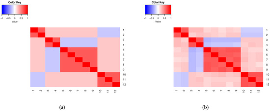
Assume six clusters ($C=6$), 12 variables ($P=12$), and $l_1=2$, $l_2=2$, $l_3=5$, and $l_4=3$. Note that $k=4$. Consider 600 subjects. We assume 12 variables to be able to demonstrate the derived dependence structure, as described by pairwise correlations, for larger and smaller homogenous groups of variables. Observations are simulated using $H=\{0.9025,0.0950,0.025\}$ and $L=\{0.0625,0.3750,0.5625\}$. In Table 1, we present the following cluster profiles created by the proposed algorithm:

• Cluster 1: $c=1$ and $k/\left(2^{c/2-0.5}\right)=4/1=4$. Then, $l_1+\dots +l_4=12$, and, according to step [5], observations from $\{1,2,3\}$ are simulated using the probabilities in vector L for all variables.
• Cluster 2: $c=2$ and $k/\left(2^{c/2-1}\right)=4/1=4$. Then, $l_1+\dots +l_4=12$, and, according to step [6], observations from $\{1,2,3\}$ are simulated using the probabilities in vector H for all variables.
• Cluster 3: $c=3$ and $k/\left(2^{c/2-0.5}\right)=4/2=2$. According to step [5], observations for the first $l_1+l_2=4$ variables are simulated using the probabilities in vector L, whilst observations for the remaining $l_3+l_4=8$ variables are simulated according to H.
• Cluster 4: $c=4$ and $k/\left(2^{c/2-1}\right)=4/2=4$. According to step [6], observations for the first $l_1+l_2=4$ variables are simulated using H, and for the remaining $l_3+l_4=8$ variables using L.
• Cluster 5: $c=5$ and $k/\left(2^{c/2-0.5}\right)=4/4=1$. According to step [5], observations for the first $l_1=2$ variables are simulated using L, for the next $l_2=2$ variables using H, for the next $l_3=5$ variables using L, and for the last $l_4=3$ variables using H.
• Cluster 6: $c=6$ and $k/\left(2^{c/2-1}\right)=4/4=1$. According to step [6], observations for the first $l_1=2$ variables are simulated using H, for the next $l_2=2$ variables using L, for the next $l_3=5$ variables using H, and for the last $l_4=3$ variables using L.

In Figure 1a, we present a heatmap of the theoretical correlations assuming interval variables, and, in Figure 1b, the sample correlations. Note that blocks of negative between-group correlations can be observed. We discuss this in detail in Section 5. The clustering of the simulated data is in accordance with the predetermined clustering; see Figure S7 in Section S4 of the Supplementary Material. This is observed in subsequent examples too, as well as in the examples in the Supplementary Material. (Throughout the manuscript, simulated subject profiles are clustered using the R package PReMiuM [11], which implements Bayesian clustering with the Dirichlet process.)

Figure 1. (a) Example 2 theoretical correlations. (b) Example 2 sample correlations.

Table 1. Cluster profiles for 12 variables ($P=12$) and 6 clusters ($C=6$) for Example 2. Observations are simulated using probability vectors L and H.

	${\mathit{x}}_{.1}$	${\mathit{x}}_{.2}$	${\mathit{x}}_{.3}$	${\mathit{x}}_{.4}$	${\mathit{x}}_{.5}$	${\mathit{x}}_{.6}$	${\mathit{x}}_{.7}$	${\mathit{x}}_{.8}$	${\mathit{x}}_{.9}$	${\mathit{x}}_{.10}$	${\mathit{x}}_{.11}$	${\mathit{x}}_{.12}$
Cluster 1	L	L	L	L	L	L	L	L	L	L	L	L
Cluster 2	H	H	H	H	H	H	H	H	H	H	H	H
Cluster 3	L	L	L	L	H	H	H	H	H	H	H	H
Cluster 4	H	H	H	H	L	L	L	L	L	L	L	L
Cluster 5	L	L	H	H	L	L	L	L	L	H	H	H
Cluster 6	H	H	L	L	H	H	H	H	H	L	L	L

Table 1. Cluster profiles for 12 variables ($P=12$) and 6 clusters ($C=6$) for Example 2. Observations are simulated using probability vectors L and H.

	${\mathit{x}}_{.1}$	${\mathit{x}}_{.2}$	${\mathit{x}}_{.3}$	${\mathit{x}}_{.4}$	${\mathit{x}}_{.5}$	${\mathit{x}}_{.6}$	${\mathit{x}}_{.7}$	${\mathit{x}}_{.8}$	${\mathit{x}}_{.9}$	${\mathit{x}}_{.10}$	${\mathit{x}}_{.11}$	${\mathit{x}}_{.12}$
Cluster 1	L	L	L	L	L	L	L	L	L	L	L	L
Cluster 2	H	H	H	H	H	H	H	H	H	H	H	H
Cluster 3	L	L	L	L	H	H	H	H	H	H	H	H
Cluster 4	H	H	H	H	L	L	L	L	L	L	L	L
Cluster 5	L	L	H	H	L	L	L	L	L	H	H	H
Cluster 6	H	H	L	L	H	H	H	H	H	L	L	L

3.2. Allowing for a Predetermined Covariance or Correlation Within Each Homogenous Group for Interval SNP-like Variables

Proposition 3.

Assume that interval variables $x_{.p}$ and $x_{.q}$ belong to the same homogenous group. For the algorithm in Section 3.1,

$$Cov(x_{.p},x_{.q})=0.25\times (f_{(p,H)}-f_{(p,L)})\times (f_{(q,H)}-f_{(q,L)}),$$

where $f_{(p,H)}={\sum }_{x_p=1}^{M_p}{x}_{p}P(x_{.p}=x_p|H_p)$ and $f_{(p,L)}={\sum }_{x_p=1}^{M_p}{x}_{p}P(x_{.p}=x_p|L_p)$.

Proof. 

See Appendix B and Appendix C. □

In practice, one may consider the simplified scenario where variables in the same homogenous group share the same set of possible values, and $(f_{(p,H)}-f_{(p,L)})=(f_{(q,H)}-f_{(q,L)})$. Then, given $\mathrm{Cov}(x_{.p},x_{.q})$, one can set cluster-specific probabilities so that, for all $x_{.p}$ in the same homogenous group,

$$\begin{array}{c}\hfill |f_{(p,H)}-f_{(p,L)}|=\sqrt{4\mathrm{Cov}(x_{.p},x_{.q})},\end{array}$$

(4)

where $|.|$ denotes the absolute value. Proposition 3 and the result above can be used for the determination of marginal covariances and correlations for interval variables with any number of levels as the proof of Proposition 3 applies generally. We now show how to utilize the results above for simulating SNP-like variables.

Application to SNP variables, given predetermined covariances:

Single Nucleotide Polymorphisms (SNPs) are observations with three levels, usually denoted by $0,1$, and 2 for ‘Wild type’, ‘Heterozygous variant’, and ‘Homozygous variant’, respectively. For an SNP $x_{.p}$, due to the Hardy–Weinberg principle [21], $P(x_{.p}=0)=p_{S_p}^2$, $P(x_{.p}=1)=2p_{S_p}(1-p_{S_p})$, and $P(x_{.p}=2)={(1-p_{S_p})}^2$, where $0<p_{S_p}<1$. Thus, $\mathrm{E}\left(x_{.p}\right|z_i=c)=2-2p_{S_p}$, $\mathrm{E}\left(x_{.p}^2\right|z_i=c)=(1-p_{S_p})(4-2p_{S_p})$, $\mathrm{Var}\left(x_{.p}\right|z_i=c)=2p_{S_p}(1-p_{S_p})$, and $f_{(p,H)}-f_{(p,L)}=\mathrm{E}\left(x_{.p}\right|p_{S_p}^H)-\mathrm{E}\left(x_{.p}\right|p_{S_p}^L)=2(p_{S_p}^H-p_{S_p}^L)$, where $p_{S_p}^H$ and $p_{S_p}^L$ are the probabilities that form the H and L SNP probability vectors.

Assume that, for $x_{.p}$ and $x_{.q}$ in the same homogenous group, $p_{S_p}^H=p_{S_q}^H$ and $p_{S_p}^L=p_{S_q}^L$, and therefore, $f_{(p,H)}=f_{(q,H)}$ and $f_{(p,L)}=f_{(q,L)}$. From (5), given a required covariance $\mathrm{Cov}(x_{.p},x_{.q})$, set cluster-specific probabilities for $x_{.p}$ and $x_{.q}$ so that $2|p_{S_p}^H-p_{S_p}^L|=\sqrt{4\mathrm{Cov}(x_{.p},x_{.q})}$. In practice, set $p_{S_p}^H=p_S^H$ to be suitably high and constant for all variables (say, $p_S^H\simeq 1$), and allow $p_{S_p}^L$ to vary in accordance with $p_S^H-p_{S_p}^L=\sqrt{\mathrm{Cov}(x_{.p},x_{.q})}$.

Example 3.

Assume six clusters ($C=6$), 12 variables ($P=12$) that emulate SNPs, and $l_1=2$, $l_2=2$, $l_3=5$, $l_4=3$. Consider 600 subjects, and $p_S^H=0.95$. Assume a covariance of 0.45 for the variables within homogenous groups. In Figure 2a, we present a heatmap of the theoretical correlation matrix for the specifications in this example, whilst sample correlations are shown in Figure 2b.

Figure 2. (a) Example 3 theoretical correlations. (b) Example 3 sample correlations.

Application to SNP variables, given predetermined correlations:

From Section 2.3, Equation (1), and for ${\psi }_1=\dots ={\psi }_C=\psi$,

$$\mathrm{Var}\left(x_{.p}\right)=\psi \sum _{c=1}^C[\mathrm{E}(x_{.p}^2|z_i=c)]-{\psi }^2{\{\sum _{c=1}^C[\mathrm{E}(x_{.p}|z_i=c)]\}}^2.$$

For an even C, for half of the clusters, $\mathrm{E}(x_{.p}^2|z_i=c)=(1-p_{S_p}^H)(4-2p_{S_p}^H)$ and $\mathrm{E}(x_{.p}|z_i=c)=2-2p_{S_p}^H$. For the remaining clusters, $\mathrm{E}(x_{.p}^2|z_i=c)=(1-p_{S_p}^L)(4-2p_{S_p}^L)$ and $\mathrm{E}(x_{.p}|z_i=c)=2-2p_{S_p}^L$. Therefore, $\mathrm{Var}\left(x_{.p}\right)$ is given by

$$\begin{array}{ccc}& \psi & [{\displaystyle \frac{C}{2}}(1-p_{S_p}^H)(4-2p_{S_p}^H)+{\displaystyle \frac{C}{2}}(1-p_{S_p}^L)(4-2p_{S_p}^L)]-{\psi }^2{[{\displaystyle \frac{C}{2}}(2-2p_{S_p}^H)+{\displaystyle \frac{C}{2}}(2-2p_{S_p}^L)]}^2\hfill \\ & =& \psi C(1-p_{S_p}^H)(2-p_{S_p}^H)+\psi C(1-p_{S_p}^L)(2-p_{S_p}^L)-{\psi }^2{C}^2{(2-p_{S_p}^H-p_{S_p}^L)}^2.\hfill \end{array}$$

Then, as $\psi =1/C$,

$$\begin{array}{ccc}& & \mathrm{Cov}(x_{.p},x_{.q})\hfill \\ & =& \mathrm{Cor}(x_{.p},x_{.q})[(1-p_{S_p}^H)(2-p_{S_p}^H)+(1-p_{S_p}^L)(2-p_{S_p}^L)-{(2-p_{S_p}^H-p_{S_p}^L)}^2].\hfill \end{array}$$

As we demonstrated earlier in this section, for a given $\mathrm{Cov}(x_{.p},x_{.q})$, $p_S^H-p_{S_p}^L=\sqrt{\mathrm{Cov}(x_{.p},x_{.q})}$. Thus, to allow for different predetermined correlations within each homogenous group of variables, one should set $p_{S_p}^H=p_S^H$ to be suitably high (say, close to 1), and let $p_{S_p}^L$ vary so that

$$\begin{array}{ccc}& & p_S^H-p_{S_p}^L\hfill \\ & =& \sqrt{Cor(x_{.p},x_{.q})}\times \sqrt{[(1-p_S^H)(2-p_S^H)+(1-p_{S_p}^L)(2-p_{S_p}^L)-{(2-p_S^H-p_{S_p}^L)}^2]}.\hfill \end{array}$$

Note that the chosen correlation is restricted so that, for $p_{S_p}^L\to 0$, the maximum possible correlation is $p_S^H$. The restriction is negligible for $\left(p_S^H\right)\simeq 1$.

Example 4.

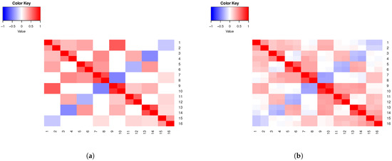
Assume eight clusters ($C=8$), 16 variables ($P=16$) that emulate SNPs, and $l_v=2$, $v=1,\dots ,8$. Consider 800 subjects, with observations simulated using $p_S^H=0.95$, for predetermined correlations within the eight homogenous groups given by $(0.4,0.5,0.6,0.7,0.8,0.6,0.7,0.4)$. In Figure 3a, we present a heatmap of the theoretical correlation matrix for the specifications in this example. In Figure 3b, we present the sample correlation matrix for the simulated observations.

Figure 3. (a) Example 4 theoretical correlations. (b) Example 4 sample correlations.

4. Genetic Profiles Defined by Correlated SNPs—A GWA Study

Data from a GWA study of lung cancer [22] are utilized. Genotyping is performed with the Illumina Sentrix HumanHap300 BeadChip, including 317,139 SNPs of subjects from the International Agency for Research on Cancer (IARC) lung cancer study. The top 200 SNPs, ranked by their p-value for association with lung cancer (adjusted for age, sex, and country) are selected. The correlation (Linkage Disequilibrium) structure is shown in Figure 4a. The selected 200 SNPs are a subset of the SNPs also analyzed in [23]. We observe 27 groups of SNPs, where SNPs are correlated within each group and uncorrelated between groups. Correlations are overwhelmingly positive. Table 2 shows the average sample correlation within each of the 27 groups for the 89 SNPs that are correlated with at least one other polymorphism.

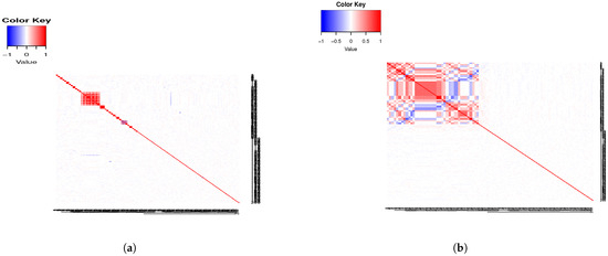
Figure 4. (a) Real data Linkage Disequilibrium. (b) Simulated data Linkage Disequilibrium.

Table 2. Average within-group sample correlations for the 89 correlated SNPs from the study of Hung et al. (2008) [22] and for the simulated data. In parentheses is the number of SNPs in each group.

Group	1 (2)	2 (2)	3 (3)	4 (2)	5 (2)	6 (3)	7 (2)	8 (2)	9 (3)	10 (2)
Corr (LD)-Real	0.68	0.96	0.62	0.91	0.96	0.93	0.90	0.98	0.91	0.98
Corr (LD)-Sim	0.69	0.96	0.63	0.90	0.96	0.93	0.90	0.98	0.91	0.98
Group	11 (2)	12 (2)	13 (21)	14 (5)	15 (2)	16 (2)	17 (3)	18 (2)	19 (3)	20 (4)
Corr (LD)-Real	0.96	0.98 *	0.59	0.94	0.32	0.92	0.41	0.96	0.63	0.66
Corr (LD)-Sim	0.96	$0.98$	0.59	0.94	0.31	0.92	0.41	0.96	0.64	0.66
Group	21 (2)	22 (7)	23 (2)	24 (3)	25 (2)	26 (2)	27 (2)
Corr (LD)-Real	0.96	${0.60}^{+}$	0.42	0.90	0.43	0.56	0.74
Corr (LD)-Sim	0.96	$0.60$	0.43	0.90	0.41	0.55	0.74

* Actual correlation is 0.99; 0.98 is used to avoid numerical instability. ⁺ Actual average correlation is 0.15; 0.6 is used after excluding negative within-group correlations.

The algorithm in Section 3.1 is used to generate a predetermined clustering structure for 6000 subjects, using simulated observations from 200 SNPs, whilst the specified homogenous groups resemble those in the real dataset. As the real dataset contains 27 groups of variables with within-group correlations that are notably non-zero, it is required that our algorithm generates 27 homogenous groups of variables, plus another group with pairwise correlations that are effectively zero. The number of homogenous groups generated by the algorithm should be a power of 2. Therefore, we consider 32 homogenous groups of SNPs that correspond to 12 predetermined clusters of subjects. For the first 27 groups, we specify within-group correlations that match the within-group correlations in the real dataset. For the last five groups, we determine a very small within-group correlation of $0.01$. This is because each one of the 111 SNPs in the last five groups corresponds to an SNP in the real data that is effectively not correlated with any other SNP. Indicatively, in the real dataset, the lower, median, and upper quartiles for the pairwise correlations of the 111 SNPs are $(-0.01,0.0001,0.01)$. The clustering structure in the simulated data is exactly as predetermined, with 12 clusters containing 500 subjects each (Supplementary Material, Section S5, Figure S8). Within-group sample correlations for the simulated data are shown in Table 2. The simulated dataset replicates almost exactly the real within-group correlations. Such control is a considerable improvement compared to the standard algorithm described in Section 2.

The Linkage Disequilibrium structure within the simulated dataset is shown in Figure 4b. We observe a notable between-group simulated correlation structure not observed in the real dataset. Figure S9 in the Supplementary Material Section S5 shows this more clearly, as the focus is on the first 99 SNPs, ignoring the last 101 uncorrelated polymorphisms. In the next section, we discuss in detail the issue of controlling between-group correlations independently of within-group correlations.

5. Discussion

5.1. Flexibility of the Proposed Algorithm

Our work concerns interval variables. The empirical evidence shows that the proposed algorithm generates a similar dependence structure for ordinal observations. The dependence structure considering nominal data differs, as negative associations are not present. Nevertheless, we observed in various examples that the overall structure of positive associations is quite similar considering interval, ordinal, and nominal variables, albeit weaker for the latter. All empirical evidence suggests that the manner in which control is effected over within-group correlations is also relevant to nominal and ordinal variables, in terms of the comparative magnitude of within-group associations. See Section S6 in the Supplementary Material for more details.

The algorithm described in Section 3 allows for a predetermined clustering structure for the subjects whilst assuming a specific stratified structure for the marginal correlations of the variables. This assumption is restrictive, as other marginal dependence structures may be observed. However, the algorithm allows the size of each one of the homogenous groups to be specified, and the value of each one of the within-group correlations. This makes it flexible enough to define a large variety of clustering and marginal dependence structures. Specifically, the user is free to define either the number of clusters C or the number of homogenous groups of variables k as a power of 2. This appears to be inflexible, as one quantity then appears to define the other through $k=2^{C/2-1}$. However, freely choosing the number of clusters only places an upper bound on the number of homogenous groups of variables. This is because correlations within some of the homogenous groups can be effectively zero.

In addition, it is not essential that C is set to be even; see Supplementary Material Section S3. We consider an even C as this creates a more distinct clustering structure. The algorithm’s flexibility is further maintained as the investigator is free to choose the number of subjects. The two sets of probabilities H and L are sufficient for defining distinct cluster profiles due to the proposed cluster profiles illustrated in Table 1. Using more than two sets of probabilities would add unnecessary complexity to the algorithm.

Cluster sizes were assumed to be equal to derive theoretical results on the algorithm’s properties, but this is not essential for the implementation of the algorithm. Empirical evidence has shown that, under unequal cluster sizes, the dependence structure between the variables created by the proposed algorithm is similar to the one derived theoretically. For one such example, see the Supplementary Material, Section S7. Comparisons between clustering approaches can be performed by using our algorithm to create datasets with a weak clustering signal, so that revealing the clustering structure is challenging. The clustering signal can be made to be weak either by considering probability vectors $L_p$ and $H_p$ that are relatively close, considering some distance metric, or by creating clusters of relatively small size, or both.

The amount of computing time required for the analyses in the main manuscript and the Supplementary Material is small. For instance, for Example 2, the calculation of theoretical correlations, plus the creation of the synthetic dataset, requires fewer than 5 s. The clustering of the subjects in the synthetic dataset created for Example 2 (as performed by the R package PReMiuM, including the post-processing phase) requires less than 1 min. In Section 4, the creation of the synthetic dataset that corresponds to the real GWA one requires less than 1 min.

5.2. Between-Group Correlations

The proposed algorithm effects control over within-group correlations. Between-group correlations are present as a direct consequence of the algorithm and the imposed clustering structure. It is the clustering structure for the subjects that determines the marginal dependence between the variables, with Proposition 3 allowing control of within-group correlations by defining probability vectors $L_p$ and $H_p$ for variable p, $p=1,\dots P$. (In a simplified set-up, we have common probability vectors L and H for all variables.) The algorithm creates a specific clustering for the subjects, with cluster profiles illustrated in Table 1 for some specific C and k. Looking at consecutive pairs of clusters in Table 1, we see a mirroring between L and H, so that, at the place where an odd cluster is determined by L (or H), the next even cluster is determined by H (or L). It is this mirroring and symmetry that create the between-group correlations.

Determination of between-group correlations independently of the within-group structure, in tandem with the predetermined clustering, is not straightforward. Equation (3) offers a direct link between the covariances $\mathrm{Cov}(x_{.p},x_{.q})$ and the variable profiles in each cluster, through $f_{p,c}$, $p=1,\dots ,P$, $c=1,\dots ,C$. P variables imply $P(P-1)/2$ covariances, under the constraint that they form a positive definite matrix. The number of different $(f_{p,c_1}-f_{p,c_2})$ quantities is $\left({\displaystyle \genfrac{}{}{0pt}{}{C}{2}}\right)P$.

It is straightforward to deduce that the number of unconstrained $(f_{p,c_1}-f_{p,c_2})$ quantities is $P(C-1)$. For predetermined covariances, (3) generates a non-linear system of $P(P-1)/2$ equations with $P(C-1)$ unknowns. Solving such a system could, in principle, allow between-group correlations to be set independently of within-group associations. However, this approach is not reliable. Numerical solutions for simple examples are not available, with no solution or an infinite number of solutions reported by the symbolic computation software MAPLE.

For a specific example, consider $P=5$, $C=2$, $\psi =0.5$, and a covariance structure so that

$$\mathrm{Cov}(x_{.1},x_{.2})=\mathrm{Cov}(x_{.1},x_{.3})=\mathrm{Cov}(x_{.2},x_{.3})=0.5,$$

$$\mathrm{Cov}(x_{.4},x_{.5})=0.6,$$

with all other covariances equal to $0.2$. This provides a system of equations with no solution according to MAPLE. A specification where $P=4$, $C=4$, $\psi =0.25$, and covariances are zero except for $\mathrm{Cov}(x_{.1},x_{.2})=\mathrm{Cov}(x_{.3},x_{.4})=0.49$ generates a system with an infinite number of solutions. Solving the system of equations produced by (3) can be problematic even when the system includes equal numbers of equations and unknowns. For instance, $P=5$ and $C=3$ create a system of equations with a Jacobian equal to zero and an infinite number of solutions. This suggests that a generally applicable algorithm, such as the one proposed in Section 3, is a suitably pragmatic approach for achieving control over the marginal dependence of the variables.

5.3. Future Work

Future work will concern additional theoretical and computational efforts to effect control over the between-group correlations that result from the proposed algorithm. Furthermore, although this is not crucial for the flexibility of the proposed algorithm, another improvement would be to relax the relation between the number of clusters C for the subjects and the number of homogenous groups k for the variables, as described by $k=2^{C/2-1}$.

References

- Müller, P.; Quintana, F.; Rosner, G.L. A Product Partition Model with Regression on Covariates. J. Comput. Graph. Stat. 2012, 20, 260–278. [Google Scholar] [CrossRef] [PubMed]
- Yau, C.; Holmes, C. Hierarchical Bayesian nonparametric mixture models for clustering with variable relevance determination. Bayesian Anal. 2011, 6, 329–352. [Google Scholar] [CrossRef] [PubMed]
- Hennig, C.; Meila, M.; Murtagh, F.; Rocci, R. Handbook of Cluster Analysis; Chapman & Hall/CRC Press: Boca Raton, FL, USA, 2015. [Google Scholar]
- Frühwirth-Schnatter, S. Finite Mixture and Markov Switching Models; Springer: Berlin/Heidelberg, Germany, 2008. [Google Scholar]
- Marbac, M.; Biernacki, C.; Vandewalle, V. Model-based clustering for conditionally correlated categorical data. arXiv 2014, arXiv:1401.5684. [Google Scholar] [CrossRef]
- Kirk, P.; Pagani, F.; Richardson, S. Bayesian outcome-guided multi-view mixture models with applications in molecular precision medicine. arXiv 2023, arXiv:2303.00318. [Google Scholar]
- Hennig, C. What are the true clusters? Pattern Recogn. Lett. 2015, 64, 53–62. [Google Scholar] [CrossRef]
- Jasra, A.; Holmes, C.C.; Stephens, D.A. Markov Chain Monte Carlo Methods and the Label Switching Problem in Bayesian Mixture Modeling. Stat. Sci. 2005, 20, 50–67. [Google Scholar] [CrossRef]
- Jing, W.; Papathomas, M.; Liverani, S. Variance Matrix Priors for Dirichlet Process Mixture Models with Gaussian Kernels. Int. Stat. Rev. 2024. early view. [Google Scholar] [CrossRef]
- Dunson, D.B.; Xing, C. Nonparametric Bayes modeling of multivariate categorical data. J. Am. Stat. Assoc. 2009, 104, 1042–1051. [Google Scholar] [CrossRef] [PubMed]
- Liverani, S.; Hastie, D.I.; Azizi, L.; Papathomas, M.; Richardson, S. PReMiuM: An R package for profile regression mixture models using Dirichlet processes. J. Stat. Softw. 2015, 64, 1–30. [Google Scholar] [CrossRef] [PubMed]
- Celeux, G.; Govaert, G. Latent class models for categorical data. In Handbook of Cluster Analysis. Handbooks of Modern Statistical Methods; Hennig, C., Meila, M., Murtagh, F., Rocci, R., Eds.; Chapman & Hall/CRC Press: Boca Raton, FL, USA, 2016; pp. 173–194. [Google Scholar]
- Oberski, D.L. Beyond the number of classes: Separating substantive from non-substantive dependence in latent class analysis. Adv. Data Anal. Classi. 2016, 10, 171–182. [Google Scholar] [CrossRef]
- Allman, E.S.; Matias, C.; Rhodes, J.A. Identifiability of parameters in latent structure models with many observed variables. Ann. Stat. 2009, 37, 3099–3132. [Google Scholar] [CrossRef]
- Bingham, S.; Riboli, E. Diet and cancer—The European prospective Investigation into cancer and nutrition. Nat. Rev. Cancer 2004, 4, 206–215. [Google Scholar] [CrossRef] [PubMed]
- Ioannidis, J.P.A.; Thomas, G.; Daly, M.J. Validating, augmenting and refining genome-wide association signals. Nat. Rev. Genet. 2009, 10, 318–329. [Google Scholar] [CrossRef] [PubMed]
- Lorenz, D.J.; Datta, S.; Harkema, S.J. Marginal association measures for clustered data. Stat. Med. 2011, 30, 3181–3191. [Google Scholar] [CrossRef] [PubMed]
- Paulou, M.; Seaman, S.R.; Copas, A.J. An examination of a method for marginal inference when the cluster size is informative. Stat. Sin. 2013, 23, 791–808. [Google Scholar]
- Wang, A.; Sabo, R.T. Simulating clustered and dependent binary variables. Austin Biom. Biostat. 2015, 2, 1020. [Google Scholar]
- Grün, B.; Malsiner-Walli, G. Bayesian finite mixture models. In Wiley StatsRef: Statistics Reference Online; Balakrishnan, N., Colton, T., Everitt, B., Piegorsch, W., Ruggeri, F., Teugels, J.L., Eds.; Wiley: Hoboken, NY, USA, 2022. [Google Scholar] [CrossRef]
- Ziegler, A.; König, I.R. A Statistical Approach to Genetic Epidemiology. Concepts and Applications; Wiley-VCH Verlag GmbH & Co.: Weinheim, Germany, 2010. [Google Scholar]
- Hung, R.J.; McKay, J.D.; Gaborieau, V.; Boffetta, P.; Hashibe, M.; Zaridze, D.; Mukeria, A.; Szeszenia-Dabrowska, N.; Lissowska, J.; Rudnai, P.; et al. A susceptibility locus for lung cancer maps to nicotinic acetylcholine receptor subunit genes on 15q25. Nature 2008, 452, 633–637. [Google Scholar] [CrossRef] [PubMed]
- Papathomas, M.; Molitor, J.; Hoggart, C.; Hastie, D.; Richardson, S. Exploring data from genetic association studies using Bayesian variable selection and the Dirichlet process: Application to searching for gene-gene patterns. Genet. Epidemiol. 2012, 36, 663–674. [Google Scholar] [CrossRef] [PubMed]
- Agresti, A. Categorical Data Analysis, 2nd ed.; John Wiley & Sons: Hoboken, NJ, USA, 2002. [Google Scholar]
- Berry, K.J.; Johnston, J.E.; Zahran, S.; Mielke, P.W., Jr. Stuart’s tau measure of effect size for ordinal variables: Some methodological considerations. Behav. Res. Methods 2009, 41, 1144–1148. [Google Scholar]
- Colwell, D.J.; Gillett, J.R. Spearman versus Kendall. Math. Gaz. 2009, 41, 1144–1148. [Google Scholar]
- Deutsch, D.; Foster, G.; Freitag, M. Ties Matter: Meta-Evaluating Modern Metrics with Pairwise Accuracy and Tie Calibration. arXiv 2023. [Google Scholar]
Disclaimer/Publisher’s Note: The statements, opinions and data contained in all publications are solely those of the individual author(s) and contributor(s) and not of MDPI and/or the editor(s). MDPI and/or the editor(s) disclaim responsibility for any injury to people or property resulting from any ideas, methods, instructions or products referred to in the content. |
© 2025 by the author. Licensee MDPI, Basel, Switzerland. This article is an open access article distributed under the terms and conditions of the Creative Commons Attribution (CC BY) license (https://creativecommons.org/licenses/by/4.0/).