Quantile Estimation Based on the Log-Skew-t Linear Regression Model: Statistical Aspects, Simulations, and Applications

Abstract

We propose a robust linear regression model assuming a log-skew-t distribution for the response variable, with the aim of exploring the association between the covariates and the quantiles of a continuous and positive response variable under skewness and heavy tails. This model includes the log-skew-normal and log-t linear regression models as special cases. Our simulation studies indicate good performance of the quantile estimation approach and its outperformance relative to the classical quantile regression model. The practical applicability of our methodology is demonstrated through an analysis of two real datasets.

1. Introduction

The classical quantile regression (Koenker and Bassett [1]) model has been widely used in situations where a comprehensive understanding of the distribution of the response variable in relation to covariates is essential. This model is given by

$$Q_{y_i}\left(\tau \right)={\mathit{x}}_i^{\prime }\mathit{\beta }\left(\tau \right),$$

(1)

for $i=1,\dots ,n$, where $Q_{y_i}\left(\tau \right)$ is the $\tau$-quantile of the random variable $Y_i$, which represents the i-th observation of the response variable Y for $0<\tau <1$. Here, $x_i$ is an r-dimensional vector containing the observed values of the i-th individual on the covariates $x_1,\dots ,x_r$, and $\mathit{\beta }\left(\tau \right)$ is a vector of regression parameters that can be estimated by solving

$$\underset{\mathit{\beta }\in {\mathbb{R}}^r}{min}\sum _{i=1}^n{\rho }_{\tau }(y_i-x_i^{\prime }\mathit{\beta }),$$

where ${\rho }_{\tau }$ is the tilted absolute value function defined as

$${\rho }_{\tau }\left(w\right)=\left\{\begin{array}{cc}\tau w,\hfill & \mathrm{if}w\ge 0,\hfill \\ (\tau -1)w,\hfill & \mathrm{if}w<0.\hfill \end{array}\right.$$

Some applications of this model include anthropometric references based on child growth curves (World Health Organization [2,3]), foreign direct investment (Chunying [4]), wage distribution (Machado andMata [5]), and ecological and biological data (Cade and Noon [6]), among many others. Quantile regression models are inherently distribution-free and robust against outlying observations in the response variable. In recent years, several parametric approaches have been proposed for modeling quantiles within the regression framework (Mazucheli et al. [7], Morán-Vásquez et al. [8,9]), which align with the direction of the present work.

This article introduces a robust linear regression model assuming a log-skew-t (LST) distribution (Marchenko and Genton [10]) for the response variable. This distribution can be obtained by applying an exponential transformation to a skew-t (ST) random variable (Azzalini and Capitanio [11]). The LST distribution has positive support and includes parameters that model skewness and heavy tails. It exhibits key statistical properties and is easily handled from a mathematical perspective, making it a valuable tool for statistical modeling. The LST distribution is suitable for modeling continuous, positive, and skewed data with potential outliers. Examples include family income data (Azzalini et al. [12]) and precipitation data (Marchenko and Genton [10]). The LST distribution includes the log-skew-normal (LSN, Morán-Vásquez et al. [9]) and log-t (LT, Morán-Vásquez and Ferrari [13]) distributions as special cases.

We provide an explicit formula for the quantiles of the LST distribution, which motivated us to propose an approach to analyzing the association between covariates and any quantile of a positive response variable by considering a regression structure on the scale parameter. To this end, we define and study the LST linear regression model (LSTLRM), which is suitable for analyzing datasets where the response variable is continuous, positive, and potentially skewed with heavy tails. This includes the LSN linear regression model (LSNLRM, Morán-Vásquez et al. [9]) and log-t linear regression model (LTLRM, Morán-Vásquez et al. [9], Vanegas and Paula [14]) as special cases. We show that the LSTLRM is equivalent to the ST linear regression model (STLRM; [11]) by applying a transformation to the response variable, which simplifies the computation of the maximum likelihood parameter estimates. We conducted simulation studies to evaluate the performance of the LSTLRM and the quantile estimators for the response variable. Additionally, we analyzed the goodness of fit of the LSTLRM through quantile–quantile plots with simulated envelopes. Finally, we applied our model to two real datasets: one concerning women’s income and the other focusing on children’s weight.

The remainder of this paper is structured as follows: Section 2 presents a brief background on the LST distribution, and a closed-form expression for its quantiles is derived. Section 3 introduces the LSTLRM, and quantile estimators for the response variable are derived. Section 4 provides Monte Carlo simulation results. Applications to women’s income data and children’s weight data are presented and discussed in Section 5. Concluding remarks are presented in Section 6.

2. Quantiles of the LST Distribution

Let $X\in \mathbb{R}$ be a random variable following a t distribution. Its probability density function (PDF) is given by

$$t(x;\xi ,\omega ,\nu )={\displaystyle \frac{\mathrm{\Gamma }\left[\right(\nu +1)/2]}{\mathrm{\Gamma }(\nu /2){\left(\pi \nu \right)}^{1/2}\omega }}{\left(1+{\displaystyle \frac{{\delta }_{\omega }(x,\xi )}{\nu }}\right)}^{-(\nu +1)/2},x\in \mathbb{R},$$

(2)

where ${\delta }_{\omega }(x,\xi )={(x-\xi )}^2/{\omega }^2$, with $\xi \in \mathbb{R}$, $\omega >0$ and $\nu >0$ denoting the location, scale, and degrees of freedom parameters, respectively. The PDF of a normal random variable $X\sim N(\xi ,{\omega }^2)$ arises as a limiting case of (2) when $\nu \to \infty$, and it is given by

$$\varphi (x;\xi ,\omega )={\left(2\pi \right)}^{-1/2}{\omega }^{-1}exp(-{\delta }_{\omega }(x,\xi )/2).$$

The PDF of an ST random variable $X\in \mathbb{R}$ is given by

$$f_{\mathrm{ST}}(x;\xi ,\omega ,\alpha ,\nu )=2t(x;\xi ,\omega ,\nu )T\left(\alpha {\omega }^{-1}(x-\xi ){\left[{\displaystyle \frac{\nu +1}{\nu +{\delta }_{\omega }(x,\xi )}}\right]}^{1/2};\nu +1\right),x\in \mathbb{R},$$

(3)

where $t(x;\xi ,\omega ,\nu )$ is the PDF defined in (2), and where $T(·;\nu )$ denotes the cumulative distribution function (CDF) of a standard t random variable with a $\nu$ degrees of freedom parameter. The parameters $\xi \in \mathbb{R}$, $\omega >0$, $\alpha \in \mathbb{R}$, and $\nu >0$ correspond to location, scale, shape, and degrees of freedom, respectively. The notation $X\sim \mathrm{ST}(\xi ,{\omega }^2,\alpha ,\nu )$ indicates that X follows the distribution with the PDF (3). The PDF of a skew-normal (SN) random variable $X\sim \mathrm{SN}(\xi ,{\omega }^2,\alpha )$ is obtained as a limiting case of (3) when $\nu \to \infty$, and it is given by

$$f_{\mathrm{SN}}(x;\xi ,\omega ,\alpha )=2\varphi (x;\xi ,\omega )\mathrm{\Phi }\left(\alpha {\omega }^{-1}(x-\xi )\right),x\in \mathbb{R},$$

where $\mathrm{\Phi }(·)$ is the standard normal CDF. Also, when $\alpha =0$ the expression in (3) simplifies to the PDF in (2). The ST distribution is useful for modeling data that exhibit skewness and heavy tails, as the parameters $\alpha$ and $\nu$ influence the skewness and the tail behavior of the distribution, respectively.

Definition 1 introduces the LST distribution as described in Azzalini et al. [12] and Marchenko and Genton [10].

Definition 1.

The positive random variable Y follows an LST distribution, denoted by $Y\sim \mathrm{LST}(\xi ,{\omega }^2,\alpha ,\nu )$, if $log\left(Y\right)\sim \mathrm{ST}(log\left(\xi \right),{\omega }^2,\alpha ,\nu )$.

From Definition 1, it is straightforward to show that the PDF of Y, $Y\sim \mathrm{LST}(\xi ,{\omega }^2,\alpha ,\nu )$, is given by

$$f_{\mathrm{LST}}(y;\xi ,\omega ,\alpha ,\nu )={\displaystyle \frac{2}{y}}t(log\left(y\right);log\left(\xi \right),\omega ,\nu )T\left(\alpha {\omega }^{-1}log\left({\displaystyle \frac{y}{\xi }}\right){\left[{\displaystyle \frac{\nu +1}{\nu +{\delta }_{\omega }(log\left(y\right),log\left(\xi \right))}}\right]}^{1/2};\nu +1\right),y>0.$$

(4)

The parameters $\xi >0$, $\alpha \in \mathbb{R}$, $\omega >0$, and $\nu >0$ correspond to scale, shape, relative dispersion, and degrees of freedom. Our parameterization differs slightly from the one used by Equation (6) of Marchenko and Genton [10], who consider in (4) a parameter $\eta \in \mathbb{R}$ instead of $log\left(\xi \right)$, which makes its interpretation more difficult. Note that the PDF in (4) has the structure

$$f_{\mathrm{LST}}(y;\xi ,\omega ,\alpha ,\nu )={\displaystyle \frac{1}{\xi }}f\left({\displaystyle \frac{y}{\xi }}\right),$$

where f is the function

$$f\left(z\right)={\displaystyle \frac{2}{z}}t(log\left(z\right);0,\omega ,\nu )T\left(\alpha {\omega }^{-1}log\left(z\right){\left[{\displaystyle \frac{\nu +1}{\nu +{\delta }_{\omega }(log\left(z\right),0)}}\right]}^{1/2};\nu +1\right),z>0.$$

This shows that $\xi$ is a scale parameter. Moreover, Definition 1, together with our parameterization, suggests a logarithmic link when a linear regression structure is considered on $\xi$, facilitating the interpretation of the regression coefficients (Section 3).

Taking the limit $\nu \to \infty$ in (4) results in the PDF of an LSN random variable $Y\sim \mathrm{LSN}(\xi ,{\omega }^2,\alpha )$ given by (Morán-Vásquez et al. [9]):

$$f_{\mathrm{LSN}}(y;\xi ,\omega ,\alpha )={\displaystyle \frac{2}{y}}\varphi (log\left(y\right);log\left(\xi \right),\omega )\mathrm{\Phi }\left(\alpha {\omega }^{-1}log\left({\displaystyle \frac{y}{\xi }}\right)\right),y>0.$$

Moreover, by setting $\alpha =0$ in (4) we retrieve the PDF of an LT random variable Y, $Y\sim \mathrm{LT}(\xi ,{\omega }^2,\nu )$, given by Morán-Vásquez and Ferrari [13], Morán-Vásquez et al. [8]

$$f_{\mathrm{LT}}(y;\xi ,\omega ,\nu )={\displaystyle \frac{1}{y}}t(log\left(y\right);log\left(\xi \right),\omega ,\nu ),y>0.$$

Figure 1 displays several shapes of the PDF in (4) for different parameter values. As shown in Figure 1a, varying values of $\xi$ change the scale of the distribution of Y, while $\omega$ influences its dispersion (Figure 1b), $\alpha$ affects its skewness (Figure 1c), and $\nu$ impacts its tail behavior (Figure 1d). It is noteworthy that smaller values of $\nu$ correspond to heavier tails in the LST distribution, and the LST distribution tends toward the LSN distribution as $\nu$ increases (Figure 1d).

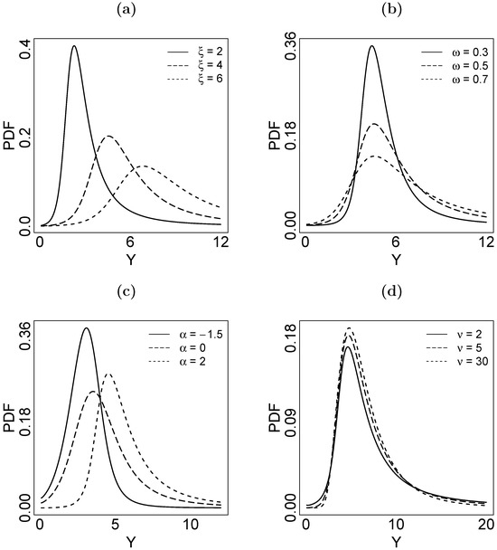
Figure 1. Graph of the PDF of the LST distribution with (a) $\omega =0.5$, $\alpha =1.5$, $\nu =3$, $\xi =2,4,6$; (b) $\xi =4$, $\alpha =1.5$, $\nu =3$, $\omega =0.3,0.5,0.7$; (c) $\xi =4$, $\omega =0.4$, $\nu =3$, $\alpha =-1.5,0,2$; (d) $\xi =4$, $\omega =0.6$, $\alpha =2$, $\nu =2,5,30$.

In Theorem 1, we derive closed-form expressions for the quantiles of the LST distribution.

Theorem 1.

Let $Y\sim \mathrm{LST}(\xi ,{\omega }^2,\alpha ,\nu )$. The τ-quantile $\begin{array}{c}\hfill Q_y\left(\tau \right)\end{array}$, $0<\tau <1$, of Y satisfies

$$\begin{array}{c}\hfill Q_y\left(\tau \right)\end{array}=\xi exp\left(\omega \begin{array}{c}\hfill Q_z\left(\tau \right)\end{array}\right),$$

(5)

with $\begin{array}{c}\hfill Q_z\left(\tau \right)\end{array}$ being the τ-quantile of the standard ST random variable $\begin{array}{c}\hfill Z\end{array}\sim \mathrm{ST}(0,1,\alpha ,\nu )$.

Proof. 

The $\tau$-quantile $\begin{array}{c}\hfill Q_y\left(\tau \right)\end{array}$, $0<\tau <1$, of $Y\sim \mathrm{LST}(\xi ,{\omega }^2,\alpha ,\nu )$ is defined as the value satisfying $P[Y\le Q_y\left(\tau \right)]=\tau$, which is equivalent to

$$P[log\left(Y\right)\le log\left(Q_y\left(\tau \right)\right)]=\tau .$$

(6)

Since $log\left(Y\right)\sim \mathrm{ST}(log\left(\xi \right),{\omega }^2,\alpha ,\nu )$, then

$$Z={\displaystyle \frac{log\left(Y\right)-log\left(\xi \right)}{\omega }}\sim \mathrm{ST}(0,1,\alpha ,\nu ).$$

Thus, in (6) we have

$$P\left(Z\le {\displaystyle \frac{log\left(Q_y\left(\tau \right)\right)-log\left(\xi \right))}{\omega }}\right)=\tau .$$

It follows from the above that $(log\left(Q_y\left(\tau \right)\right)-log\left(\xi \right))/\omega$ is the $\tau$-quantile of $Z\sim \mathrm{ST}(0,1,\alpha ,\nu )$; that is,

$$Q_z\left(\tau \right)={\displaystyle \frac{log\left(Q_y\left(\tau \right)\right)-log\left(\xi \right))}{\omega }}.$$

Finally, solving for $Q_y\left(\tau \right)$ from the above expression, we obtain the desired result.  □

Equation (5) shows that any quantile of Y, $Y\sim \mathrm{LST}(\xi ,{\omega }^2,\alpha ,\nu )$ is proportional to $\xi$. Thus, by considering a regression structure on $\xi$ we can model any quantile of Y through a set of covariates (Section 3).

In order to establish an interpretation for $\omega$, we consider a robust coefficient of variation of $\begin{array}{c}\hfill Y\sim \mathrm{LST}(\xi ,{\omega }^2,\alpha ,\nu )\end{array}$ based on quantiles, as proposed by Rigby and Stasinopoulos [15]:

$${\mathrm{CV}}_Y={\displaystyle \frac{3}{4}}\begin{array}{c}\hfill \left({\displaystyle \frac{Q_y(3/4)-Q_y(1/4)}{Q_y(1/2)}}\right)\end{array}.$$

(7)

Substituting (5) into (7), we obtain

$${\mathrm{CV}}_Y={\displaystyle \frac{3}{4}}\begin{array}{c}\hfill \left({\displaystyle \frac{exp\left(Q_z(3/4)\omega \right)-exp\left(Q_z(1/4)\omega \right)}{exp\left(Q_z(1/2)\omega \right)}}\right)\end{array}.$$

The above expression indicates that ${\mathrm{CV}}_Y$ is a non-decreasing function of $\omega$, and, therefore, we can conclude that $\omega$ is a parameter that influences the relative dispersion of the distribution of Y.

Finally, it is straightforward to show that if $Y\sim \mathrm{LST}(\xi ,{\omega }^2,\alpha ,\nu )$ then

$${\delta }_{\omega }(log\left(Y\right),log\left(\xi \right))\sim F_{1,\nu },$$

(8)

where $F_{{\nu }_1,{\nu }_2}$ represents the F-distribution with ${\nu }_1$ and ${\nu }_2$ degrees of freedom. This expression will be important for establishing a diagnostic tool for the LSTLRM (Section 3).

3. Quantile Estimation Using the LSTLRM

In this section, we introduce the LSTLRM, with the aim of describing the association between the quantiles of a random variable following an LST distribution and the covariates.

Assume that $Y_1,\dots ,Y_n$ are independent random variables representing observations of a positive response variable Y across n individuals. We define the LSTLRM as

$$\left\{\begin{array}{c}{Y}_i\stackrel{\mathrm{ind}}{\sim }\mathrm{LST}({\xi }_i,{\omega }^2,\alpha ,\nu ),\hfill \\ log\left({\xi }_i\right)={\mathit{x}}_i^{\prime }\mathit{\beta },\hfill \end{array}\right.$$

(9)

for $i=1,\dots ,n$, where “ind” means “independent”. Note that ${\xi }_i$ may vary across observations. The constant vector $x_i={(x_{i1},\dots ,x_{ir})}^{\prime }$ consists of the values of the covariates $x_1,\dots ,x_r$ for the i-th individual. Let us suppose that $x_{i1}=1$ for $i=1,\dots ,n$, in order to include an intercept in the model. The vector $\mathit{\beta }={({\beta }_1,\dots ,{\beta }_r)}^{\prime }$ consists of the regression coefficients, while $\omega >0$, $\alpha \in \mathbb{R}$, and $\nu >0$ denote the relative dispersion, shape, and degrees of freedom parameters, respectively. The LSTLRM (9) involves $k=r+3$ parameters in total.

If $\nu \to \infty$ in (9), we obtain the LSNLRM given by Morán-Vásquez et al. [9],

$$\left\{\begin{array}{c}{Y}_i\stackrel{\mathrm{ind}}{\sim }\mathrm{LSN}({\xi }_i,{\omega }^2,\alpha ),\hfill \\ log\left({\xi }_i\right)={\mathit{x}}_i^{\prime }\mathit{\beta },\hfill \end{array}\right.$$

for $i=1,\dots ,n$. When $\alpha =0$ in (9), we retrieve the LTLRM (Morán-Vásquez et al. [9], Vanegas and Paula [14]) given by

$$\left\{\begin{array}{c}{Y}_i\stackrel{\mathrm{ind}}{\sim }\mathrm{LT}({\xi }_i,{\omega }^2,\nu ),\hfill \\ log\left({\xi }_i\right)={\mathit{x}}_i^{\prime }\mathit{\beta },\hfill \end{array}\right.$$

for $i=1,\dots ,n$.

Equations (5) and (9) allow us to relate any $\tau$-quantile, $Q_{y_i}\left(\tau \right)$, of $Y_i$ to the set of covariates $x_1,\dots ,x_r$ through a linear regression structure. In fact,

$$Q_{y_i}\left(\tau \right)=exp\left(\sum _{j=1}^r{\beta }_j{x}_{ij}+\omega Q_z\left(\tau \right)\right),$$

(10)

for $i=1,\dots ,n$, where $Q_z\left(\tau \right)$ is the $\tau$-quantile of the standard ST random variable $\begin{array}{c}\hfill Z\end{array}\sim \mathrm{ST}(0,1,\alpha ,\nu )$. It is evident that $exp\left({\beta }_j\right)$ indicates the multiplicative change in $\begin{array}{c}\hfill Q_y\left(\tau \right)\end{array}$ resulting from a one-unit increase in $x_j$, holding all other covariates constant. Moreover, the variation in $\begin{array}{c}\hfill Q_y\left(\tau \right)\end{array}$ is controlled by $\begin{array}{c}\hfill Q_z\left(\tau \right)\end{array}$ and scaled by $\omega$. It is worth noting that the estimation of multiple quantiles of Y can be achieved by fitting the LSTLRM (9) once, along with separate calculations of the quantiles of the standard ST distribution.

From Definition 1, we know that the LSTLRM (9) can be equivalently expressed as

$$log\left(Y_i\right)\stackrel{\mathrm{ind}}{\sim }\mathrm{ST}({\mathit{x}}_i^{\prime }\mathit{\beta },{\omega }^2,\alpha ,\nu ).$$

(11)

For this reason, the parameters $\mathit{\theta }={({\mathit{\beta }}^{\prime },\omega ,\alpha ,\nu )}^{\prime }$ involved in the LSTLRM can be estimated using the STLRM (Section 4.3 of Azzalini and Capitanio [11]) with log-transformed responses. We denote by $\widehat{\mathit{\theta }}={({\widehat{\mathit{\beta }}}^{\prime },\widehat{\omega },\widehat{\alpha },\widehat{\nu })}^{\prime }$ the maximum likelihood estimator of $\mathit{\theta }$. From (10), we obtain the maximum likelihood estimator of the $\tau$-quantile of $Y_i$, for $0<\tau <1$, denoted by ${\widehat{Q}}_{y_i}\left(\tau \right)$, as

$${\widehat{Q}}_{y_i}\left(\tau \right)=exp\left(\sum _{j=1}^r{\widehat{\beta }}_j{x}_{ij}+\widehat{\omega }{\widehat{Q}}_z\left(\tau \right)\right),$$

(12)

where $\begin{array}{c}\hfill {\widehat{Q}}_z\left(\tau \right)\end{array}$ is the estimated $\tau$-quantile of the standard ST random variable $\begin{array}{c}\hfill Z\end{array}\sim \mathrm{ST}(0,1,\widehat{\alpha },\widehat{\nu })$.

Let $y_1,\dots ,y_n$ represent the observations from the independent random variables as specified in (9). The log-likelihood function of $\mathit{\theta }$ is given by

$$\mathcal{l}\left(\mathit{\theta }\right)=\sum _{i=1}^n{\mathcal{l}}_i\left(\mathit{\theta }\right),$$

(13)

where ${\mathcal{l}}_i\left(\mathit{\theta }\right)$ represents the log-likelihood contribution of the i-th observation, and it is given by

$$\begin{array}{cc}\hfill {\mathcal{l}}_i\left(\mathit{\theta }\right)& =C-log\left(\omega \right)-{\displaystyle \frac{1}{2}}log\left(\nu \right)+log\left(\mathrm{\Gamma }\left({\displaystyle \frac{\nu +1}{2}}\right)\right)-log\left(\mathrm{\Gamma }\left({\displaystyle \frac{\nu }{2}}\right)\right)-{\displaystyle \frac{\nu +1}{2}}log\left(1+{\displaystyle \frac{{\delta }_{\omega }(log\left(y_i\right),{\mathit{x}}_i^{\prime }\mathit{\beta })}{\nu }}\right)\hfill \\ \hfill & +log\left(T\left(\alpha {\omega }^{-1}(log\left(y_i\right)-{\mathit{x}}_i^{\prime }\mathit{\beta }){\left[{\displaystyle \frac{\nu +1}{\nu +{\delta }_{\omega }(log\left(y_i\right),{\mathit{x}}_i^{\prime }\mathit{\beta })}}\right]}^{1/2};\nu +1\right)\right),\hfill \end{array}$$

for $i=1,\dots ,n$, where C is constant with respect to $\mathit{\theta }$. The above log-likelihood function is equivalent to the univariate case of the formulation given in Equation (6.33) of Azzalini and Capitanio [11], with log-transformed response observations. The score vector with respect to $\mathit{\theta }$ and the observed information matrix is studied in Section 4.3.3 of Azzalini and Capitanio [11]. The estimator $\widehat{\mathit{\theta }}$ does not have a closed-form expression, so it is approximated using computational methods implemented in the sn package (Azzalini [16]) in R. This package also computes the observed information matrix, from which the estimated asymptotic covariance matrix of $\widehat{\mathit{\theta }}$ is obtained, enabling the implementation of inferential procedures for the model parameters.

An asymptotic $100(1-\rho )\%$, $0<\rho <1$ confidence interval for ${\mathit{\beta }}_j$ is given by

$${\widehat{\mathit{\beta }}}_j\pm z_{1-\rho /2}\widehat{\mathrm{S}\mathrm{E}}\left({\widehat{\mathit{\beta }}}_j\right),$$

with $z_{1-\rho /2}$ denoting the $(1-\rho /2)$-quantile of the standard normal distribution and $\widehat{\mathrm{S}\mathrm{E}}\left({\widehat{\mathit{\beta }}}_j\right)$ denoting the estimated asymptotic standard error of ${\widehat{\mathit{\beta }}}_j$ obtained from the estimated asymptotic covariance matrix. This confidence interval can be used to assess the statistical significance of $x_j$ in the response variable Y. We consider the hypothesis ${\mathrm{H}}_0:{\mathit{\beta }}_j=0$ against ${\mathrm{H}}_1:{\mathit{\beta }}_j\ne 0$ to test the significance of ${\mathit{\beta }}_j$. If ${\mathrm{H}}_0$ is not rejected then $x_j$ can be omitted from the model. The Wald statistic for this hypothesis is

$$W={\left({\displaystyle \frac{{\widehat{\mathit{\beta }}}_j}{\widehat{\mathrm{S}\mathrm{E}}\left({\widehat{\mathit{\beta }}}_j\right)}}\right)}^2,$$

which asymptotically follows a chi-squared distribution with one degree of freedom.

To select models, we use the Akaike information criterion (AIC), defined as

$$\mathrm{AIC}=-2\mathcal{l}\left(\widehat{\mathit{\theta }}\right)+2k.$$

Among the candidate models, the one with the lowest AIC is considered to offer the best fit to the data. We also display quantile–quantile plots to assess the model fit. These plots allow us to compare the observed quantiles ${\widehat{r}}_i^2={\delta }_{\widehat{\omega }}(log\left(y_i\right),{\mathit{x}}_i^{\prime }\widehat{\beta }))$, $i=1,\dots ,n$ with the theoretical quantiles $r_{{\alpha }_i}^2=F_{1,\widehat{\nu }}^{-1}\left({\alpha }_i\right)$, $i=1,\dots ,n$, where $F_{1,\widehat{\nu }}$ is the CDF of an F-distribution with 1 and $\widehat{\nu }$ degrees of freedom; see Equation (8). We consider ${\alpha }_i=i/(n+1)$, $i=1,\dots ,n$. Additionally, simulated envelopes (Atkinson [17]) are added to the quantile–quantile plots to facilitate a more rigorous comparison between the observed and theoretical quantiles, thereby aiding in the evaluation of the model fit. The construction of the simulated envelopes based on our model is described in the following steps:

1.

Generate a random sample, $z_1,\dots ,z_n$, of $Z\sim \mathrm{ST}(0,1,\widehat{\alpha },\widehat{\nu })$.

2.

Calculate $r_i^2=z_i^2$, $i=1,\dots ,n$.

3.

Perform steps 1 and 2 m times to yield $r_{ij}^2$, $i=1,\dots ,n$, $j=1,\dots ,m$.

4.

Calculate $r_{\left(i\right)\mathrm{L}}^2=min\{r_{i1}^2,\dots ,r_{im}^2\}$ and $r_{\left(i\right)\mathrm{U}}^2=max\{r_{i1}^2,\dots ,r_{im}^2\}$, for $i=1,\dots ,n$.

5.

The lower and upper bounds of ${\widehat{r}}_i^2$ are $r_{\left(i\right)\mathrm{L}}^2$ and $r_{\left(i\right)\mathrm{U}}^2$, respectively.

We also adopt the residual diagnostics illustrated in Azzalini and Capitanio [18] and Riani et al. [19] as further evidence of the agreement between the data and the LSTLRM, by plotting the histogram of the residuals $e_i=log\left(y_i\right)-{\mathit{x}}_i^{\prime }\widehat{\mathit{\beta }}$, $i=1,\dots ,n$, with the PDF of $X\sim \mathrm{ST}(0,{\widehat{\omega }}^2,\widehat{\alpha },\widehat{\nu })$ superimposed.

4. Simulation Studies

This section presents simulation studies to illustrate the performance of the parameter estimation method for the LSTMRL model (Equation (9)) and the quantile modeling approach proposed in Equation (12). To carry out the simulations, we considered the model

$$\left\{\begin{array}{c}{Y}_i\stackrel{ind}{\sim }\mathrm{LST}({\xi }_i,{\omega }^2,\alpha ,\nu ),\hfill \\ log\left({\xi }_i\right)={\mathit{\beta }}_1+{\mathit{\beta }}_2{x}_{i2}+{\mathit{\beta }}_3{x}_{i3},\hfill \end{array}\right.$$

(14)

for $i=1,\dots ,n$. The simulation studies were conducted using sample sizes n = 50, 100, 500, 1000, with $10,000$ Monte Carlo replicates. In order to calculate the true parameters for conducting the simulations, we fitted the LSTLRM (14) to the women’s income data, where the response variable Y and the covariates $x_1$ and $x_2$ are described in Section 5.1. The values of the true parameters are shown in the first column of Table 1. The covariate values $x_{ij}$, $i=1,\dots ,n$, $j=1,2$ were obtained as independent random draws from different distributions and remained constant throughout the simulation process. These distributions were selected using the fitdistr function from the MASS package in the R software 4.5.0. Consequently, $x_2$ was generated from a Gamma distribution with shape parameter $11.6$ and rate parameter $0.3$, and $x_3$ was generated from a Weibull distribution with shape parameter $4.4$ and scale parameter $13.9$.

Table 1. Summary statistics of the estimated parameters; LSTLRM.

		$\mathit{n}=50$		$\mathit{n}=100$		$\mathit{n}=500$		$\mathit{n}=1000$
True Parameter		Median	MAD	Median	MAD	Median	MAD	Median	MAD
${\mathit{\beta }}_1$	−1.4863	−1.5029	0.2625	−1.4881	0.1714	−1.4861	0.0797	−1.4847	0.0549
${\mathit{\beta }}_2$	0.0141	0.0140	0.0034	0.0141	0.0028	0.0141	0.0012	0.0141	0.0009
${\mathit{\beta }}_3$	0.1032	0.1029	0.0147	0.1035	0.0086	0.1033	0.0040	0.1032	0.0029
$\omega$	0.4230	0.4144	0.0812	0.4253	0.0624	0.4239	0.0266	0.4231	0.0191
$\alpha$	−0.8377	−0.8706	0.6470	−0.9111	0.4463	−0.8544	0.1768	−0.8458	0.1254
$\nu$	3.3462	3.3163	1.1832	3.5137	0.9473	3.3943	0.3800	3.3613	0.2684

We used the selm.fit function from the sn package in R to fit the LSTLRM model (14) at each iteration. The nlminb optimization algorithm was employed in each simulation experiment to maximize the log-likelihood function (13). The selection of initial parameter values for the maximum likelihood estimation is described in detail in Section 3.3 of Azzalini and Salehi [20], and it was implemented in the subroutine st.prelimFit, which is known as the selm.fit function. We used a tolerance level of ${10}^{-10}$ for the relative change in the log-likelihood as a convergence criterion. If this criterion is not met, the algorithm will run for a maximum of 2000 iterations.

We report robust summaries (the median and the median absolute deviation (MAD)) of the estimates in Table 1 and Table 2, since the degrees of freedom parameter estimates can take large values for certain samples, which affects traditional statistics commonly used in simulation studies, such as the mean and the root mean squared error. The results shown in Table 1 suggest desirable properties of the parameter estimators of the LSTLRM (14), with medians closely approximating the true parameter values and the MAD decreasing as the sample size increased. For $n=50$ and $n=100$, convergence was achieved in $78.06\%$ and $97.13\%$ of the samples, respectively, whereas for $n=500$ and $n=1000$, convergence was achieved in $100\%$ of the samples.

Table 2. Median and MAD of estimated quantiles; LSTLRM and classical QR.

		$\mathit{n}=50$				$\mathit{n}=100$				$\mathit{n}=500$				$\mathit{n}=1000$
		LSTLRM		QR		LSTLRM		QR		LSTLRM		QR		LSTLRM		QR
True Quantile		Median	MAD	Median	MAD	Median	MAD	Median	MAD	Median	MAD	Median	MAD	Median	MAD	Median	MAD
$\begin{array}{c}\hfill Q_y\left(0.03\right)\end{array}$	0.3135	0.3346	0.0786	0.3727	0.0890	0.3037	0.0491	0.3306	0.0629	0.3268	0.0242	0.3477	0.0330	0.2935	0.0157	0.3124	0.0205
$\begin{array}{c}\hfill Q_y\left(0.05\right)\end{array}$	0.4074	0.4315	0.0723	0.4602	0.0877	0.3895	0.0448	0.4167	0.0587	0.4233	0.0221	0.4481	0.0290	0.3806	0.0144	0.4039	0.0185
$\begin{array}{c}\hfill Q_y\left(0.25\right)\end{array}$	0.8139	0.8404	0.0505	0.8837	0.0607	0.7608	0.0329	0.8086	0.0400	0.8409	0.0158	0.8894	0.0194	0.7592	0.0103	0.8053	0.0123
$\begin{array}{c}\hfill Q_y\left(0.50\right)\end{array}$	1.1030	1.1272	0.0496	1.1906	0.0603	1.0282	0.0314	1.0976	0.0398	1.1386	0.0156	1.2094	0.0197	1.0286	0.0104	1.0960	0.0123
$\begin{array}{c}\hfill Q_y\left(0.75\right)\end{array}$	1.4318	1.4476	0.0676	1.5550	0.0843	1.3308	0.0426	1.4362	0.0546	1.4769	0.0209	1.5827	0.0274	1.3347	0.0141	1.4358	0.0169
$\begin{array}{c}\hfill Q_y\left(0.95\right)\end{array}$	2.2065	2.1891	0.2087	2.4660	0.3065	2.0197	0.1348	2.2466	0.1910	2.2674	0.0681	2.4698	0.0933	2.0534	0.0449	2.2528	0.0594
$\begin{array}{c}\hfill Q_y\left(0.97\right)\end{array}$	2.5431	2.5097	0.3168	2.8332	0.4771	2.3094	0.2052	2.5879	0.3067	2.6075	0.1063	2.8533	0.1500	2.3639	0.0701	2.6083	0.0947

Next, we computed the true quantiles $\begin{array}{c}\hfill Q_y\left(\tau \right)\end{array}$ for $\tau =0.03, 0.05, 0.25, 0.50, 0.75, 0.95, 0.97$ by substituting the true parameter values into the quantile response function associated with Equation (10). Specifically,

$$\begin{array}{c}\hfill Q_y\left(\tau \right)\end{array}=exp(-1.4863+0.0141x_1+0.1032x_2+0.4230\begin{array}{c}\hfill Q_z\left(\tau \right)\end{array}),$$

(15)

where $\begin{array}{c}\hfill Q_z\left(\tau \right)\end{array}$ is the $\tau$-quantile of the standard ST random variable $\begin{array}{c}\hfill Z\end{array}\sim \mathrm{ST}(0,1,-0.8377,3.3462)$. The values of $x_1$ and $x_2$ were replaced with their respective sample means, ${\overline{x}}_1=35.87$ and ${\overline{x}}_2=12.66$, computed from the covariates in the women’s income dataset described in Section 5.1. Substituting these values into Equation (15), we obtained

$$Q_y\left(\tau \right)=exp(0.3259+0.4230Q_z\left(\tau \right)).$$

For each simulated sample, we computed $\begin{array}{c}\hfill {\widehat{Q}}_y\left(\tau \right)\end{array}$ using Equation (12), where the covariates $x_1$ and $x_2$ were replaced by the sample means computed from the simulated values of $x_1$ and $x_2$; that is, ${\overline{x}}_j={\displaystyle \frac{1}{n}}{\sum }_{i=1}^n{x}_{ij}$ for $j=1,2$. The figures in Table 2 reveal that the quantile estimators provided by (1) and (12) performed well, as the medians closely approximated the true quantiles and the MAD became smaller with increasing sample size. However, note that in all cases the quantile estimates under our model yielded smaller MAD values in comparison to those provided by (1). Therefore, our model provides more accurate estimates than the classical quantile regression model. All computational procedures were carried out using the R programming language [21], version 4.4.1. All results are fully reproducible using the code available at https://github.com/moranvasquez/LSTLRM, accessed on 23 June 2025.

5. Data Analyses

For this section, we analyzed two datasets with the aim of demonstrating the usefulness of estimating quantiles using the LSTLRM in various contexts. In the first dataset, we modeled quantiles of women’s income based on years of schooling and age. In the second dataset, we constructed reference quantile charts for children’s weight based on gender and age.

5.1. Women’s Income Data

Women’s participation in the labor market has been a topic of interest for a long time. Analyzing women’s income data is crucial for understanding the economic, political, and social factors that contribute to gender inequalities and the wage gap, while also informing the design of public policies that promote pay equity and the well-being of women (de Castro Romero et al. [22]). Several studies have examined variables that affect the distribution of women’s income, such as education level, age, and the number of children (Arellano-Valle et al. [23]). On the other hand, the distribution of income data typically exhibits skewness and heavy tails (Cowell and Victoria-Feser [24], Saulo et al. [25]), and several economic aspects can be studied from this distribution if there is a complete understanding of it, which can be achieved by modeling quantiles (Altonji [26], Card and Lemieux [27]).

We analyzed women’s income data collected in 2021 from the Gran Encuesta Integrada de Hogares (DANE [28]). The data consisted of 770 women aged 18 to 57 years from Rionegro municipality, Antioquia department, Colombia. We considered the income received in the last month (in COP millions) as a response variable, and age (A; in years) and years of schooling (S; in years) as covariates. Figure 2 presents boxplots of the women’s income based on age (Figure 2a) and years of schooling (Figure 2b). Note that the empirical quartiles of the women’s income were affected by age and years of schooling. Moreover, the women’s income showed skewness and outliers. To analyze the relationship between these variables, we fitted the following LSTLRM,

$$\left\{\begin{array}{c}{Y}_i\stackrel{ind}{\sim }\mathrm{LST}({\xi }_i,{\omega }^2,\alpha ,\nu ),\hfill \\ log\left({\xi }_i\right)={\beta }_1+{\beta }_2{A}_i+{\beta }_3{S}_i,\hfill \end{array}\right.$$

(16)

for $i=1,\dots ,770$.

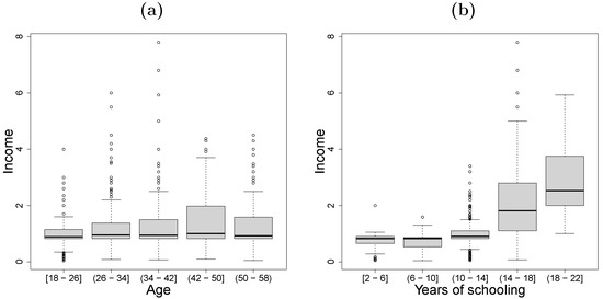
Figure 2. Boxplots of (a) women’s income vs. age, (b) women’s income vs. years of schooling.

With the aim of evaluating the simultaneous control of skewness and tail behavior through the parameters $\alpha$ and $\nu$, respectively, we fitted the LSTLRM and LSNLRM and compared their performance. The AIC values for the LSTLRM and LSNLRM were $1143.96$ and $1228.63$, respectively. Based on these values, and on the quantile–quantile plots with simulated envelopes shown in Figure 3, we concluded that the LSTLRM provided the best fit to the women’s income data.

Figure 3. Quantile–quantile plots of square normalized residuals with simulated envelope for (a) LSNLRM, (b) LSTLRM; women’s income data.

Table 3 presents the maximum likelihood estimates of ${\mathit{\beta }}_1$, ${\mathit{\beta }}_2$, and ${\mathit{\beta }}_3$, along with their corresponding asymptotic standard errors (SE), $95\%$ confidence intervals, and the p-values from the Wald test for testing ${\mathrm{H}}_0:{\mathit{\beta }}_j=0$ against ${\mathrm{H}}_1:{\mathit{\beta }}_j\ne 0$, for $j=1,2,3$. It is important to note that all covariates are significant in the LSTLRM. The maximum likelihood estimates for the parameters of relative dispersion, shape, and degrees of freedom, along with their respective standard errors in parentheses, were as follows: $\widehat{\omega }=0.4230\left(0.0386\right)$, $\widehat{\alpha }=-0.8377\left(0.2371\right)$, and $\widehat{\nu }=3.3462\left(0.4706\right)$, respectively. The asymptotic $95\%$ confidence interval for $\alpha$ was $(-1.3024,-0.3730)$, which did not contain zero. Moreover, the likelihood ratio test for the hypothesis ${\mathrm{H}}_0:\alpha =0$ against ${\mathrm{H}}_1:\alpha \ne 0$ yielded a p-value less than ${10}^{-8}$. Therefore, we concluded that the shape parameter was significantly different from zero. As a result, we did not assume an LTLRM for the women’s income data. The histogram of the residuals $e_i$, $i=1,\dots ,n$ in Figure 4 overlaid with the PDF of $X\sim \mathrm{ST}(0,0.1789,-0.8377,3.3462)$ together with Figure 3b indicates a good fit of the LSTLRM to the women’s income data.

Table 3. Results from fitting the LSTLRM to the women’s income data.

Covariate	Estimate	SE	Lower	Upper	p-Value
Intercept	−1.4863	0.0927	−1.6679	−1.3047	<0.0001
Age	0.0141	0.0016	0.0110	0.0171	<0.0001
Years of schooling	0.1032	0.0052	0.0930	0.1134	<0.0001

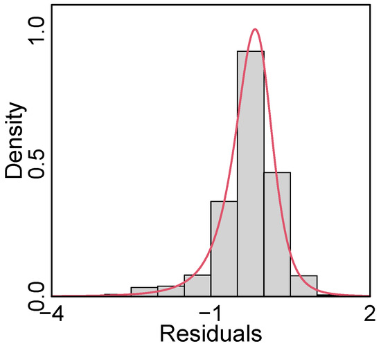
Figure 4. Histogram of the residuals overlaid with the PDF of the ST distribution; women’s income data.

Figure 5 displays the estimated quartiles of the women’s income as a function of years of schooling, overlaid on the data, for ages 25 (Figure 5a), 35 (Figure 5b), 45 (Figure 5c), and 55 (Figure 5d). We can observe that the income quartiles increased as the years of schooling increased. As expected, the relationship between income and years of schooling was affected by age. For the younger women, income was more homogeneous, while for the older women income showed greater heterogeneity. We also observe that the women with fewer years of schooling tended to have more homogeneous income than the women with more years of schooling. Additionally, we can conclude that the younger women tended to have lower incomes, even though they had the same number of years of schooling as the older women.

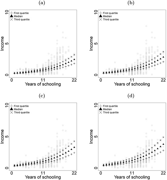
Figure 5. Estimated quartiles for women’s income by years of schooling at ages (a) 25 years, (b) 35 years, (c) 45 years, (d) 55 years.

5.2. Children’s Weight Data

We applied the LSTLRM to build reference quantile curves for children’s weight as a function of gender and age. The analysis relied on a sample of 3663 children (1728 girls and 1935 boys) aged from 2 to 5 years (inclusive), which was collected in 2018 in the Buenos Aires neighborhood of the municipality of Medellín, Colombia (MEDATA [29]). The response variable Y corresponded to the child’s weight (in kilograms), and the covariates G and A corresponded to gender (0 for girls and 1 for boys) and age (in years), respectively. Morán-Vásquez et al. [9] provide motivations and an exploratory analysis based on the aforementioned data, and they present an application in the building of reference curves using the LSNLRM. For this paper, we constructed reference curves via the LSTLRM and compared the fit with the LSNLRM. For this purpose, we considered the model

$$\left\{\begin{array}{c}{Y}_i\stackrel{ind}{\sim }\mathrm{LST}({\xi }_i,{\omega }^2,\alpha ,\nu ),\hfill \\ log\left({\xi }_i\right)={\mathit{\beta }}_1+{\mathit{\beta }}_2{G}_i+{\mathit{\beta }}_3{A}_i,\hfill \end{array}\right.$$

(17)

for $i=1,\dots ,3663$. Figure 6 suggests that both models exhibited a good fit to the children’s weight data. However, the AIC value for the LSTLRM was $-4931.84$, whereas that of the LSNLRM was $-4915.05$. Therefore, we selected the LSTLRM as the better model, which included the degrees of freedom parameter.

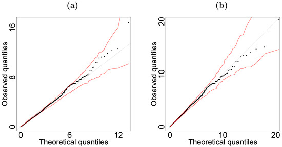
Figure 6. Quantile-quantile plots of square normalized residuals with simulated envelope for (a) LSNLRM, (b) LSTLRM; children’s weight data.

The values in Table 4 show that all the covariates were significant in the LSTLRM. The maximum likelihood estimates, along with their respective standard errors, for the remaining parameters were $\widehat{\omega }=0.1421\left(0.0062\right)$, $\widehat{\alpha }=1.0488\left(0.1415\right)$, and $\widehat{\nu }=17.4193\left(4.4635\right)$. The asymptotic $95\%$ confidence interval for $\alpha$ was $(0.7715,1.3262)$, and the p-value obtained from the likelihood ratio test for the hypothesis ${\mathrm{H}}_0:\alpha =0$ against ${\mathrm{H}}_1:\alpha \ne 0$ was less than ${10}^{-22}$. These results indicate that the shape parameter was significantly different from zero, implying that the LTLRM was not appropriate for modeling the children’s weight data. Figure 7 presents the histogram of the residuals $e_i$, $i=1,\dots ,n$ overlaid with the PDF of $X\sim \mathrm{ST}(0,0.1421,1.0488,17.4193)$. In conjunction with the plot shown in Figure 6b, this supports the suitability of the LSTLRM for modeling the children’s weight data.

Table 4. Results from fitting the LSTLRM to the children’s weight data.

Explanatory Variable	Estimate	SE	Lower	Upper	p-Value
Intercept	2.0984	0.0114	2.0761	2.1207	<0.0001
Gender	0.0233	0.0040	0.0154	0.0312	<0.0001
Age	0.1425	0.0023	0.1380	0.1470	<0.0001

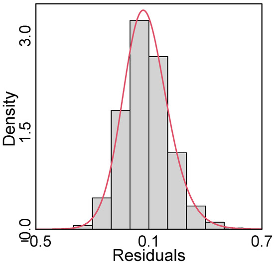
Figure 7. Histogram of the residuals overlaid with the PDF of the ST distribution; children’s weight data.

Figure 8 displays the fitted quantile curves at the percentiles $0.03$, $0.05$, $0.25$, $0.50$, $0.75$, $0.95$, and $0.97$ overlaid on the scatterplot of the children’s weight versus their age for both the girls and boys. These reference percentile curves serve as a tool to assess and monitor infant growth based on weight, helping prevent nutritional and developmental problems (Gidi et al. [30], Paulsen et al. [31]). Although this analysis was conducted using the LSTLRM, the results are similar to those obtained under the LSNLRM (Section 5 of Morán-Vásquez et al. [9]), which we expected, given that the estimate of the degrees of freedom parameter was large.

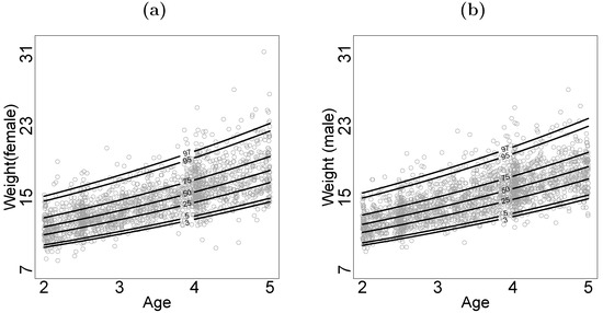
Figure 8. Estimated quantile curves for children’s weight by age: (a) girls, (b) boys.

6. Final Remarks

In this work, we propose the LSTLRM, which is a robust approach based on the LST distribution. This model provides a flexible framework for estimating quantiles of continuous, positive response variables, particularly in settings characterized by skewness and heavy tails. Our motivation for studying the LSTLRM was the proportional relationship between any quantile of the LST distribution and the scale parameter $\xi$. Furthermore, the connection between the LSTLRM and the STLRM enables maximum likelihood estimation, supports inferential procedures, and facilitates the assessment of goodness of fit. Our model generalizes previous approaches, such as the LSNLRM and the LTLRM, offering greater flexibility for modeling various data characteristics.

Our simulation studies confirmed the satisfactory performance of the parameter estimators and the quantile estimation methodology. Furthermore, a comparison with the classical quantile regression model showed that our model provides more accurate estimates. We illustrated the usefulness of our model through its applications to women’s income data and children’s weight data. In both cases, the LSTLRM provided a better fit than the LSNLRM, highlighting the importance of modeling skewness and heavy tails in the response variable. Based on the fitted models, we provided estimated quantiles that facilitated analysis of the distribution of the women’s income across years of schooling and age and enabled the construction of growth curves for the children’s weight as a function of age and gender. The goodness of fit of our models was assessed using quantile–quantile plots of squared normalized residuals with simulated envelopes and histograms of residuals with overlaid PDFs. Additionally, we performed likelihood ratio tests to compare the LSTLRM with the LTLRM, concluding in both applications that the LTLRM was not supported. Reproduction of the results in this paper is possible with the code accessible at https://github.com/moranvasquez/LSTLRM, accessed on 23 June 2025.

Additional diagnostic procedures for the LSTLRM will be addressed in future research, as well as regression models based on the LST distribution that handle incomplete data, measurement error, and mixed models. It would also be of interest to study multivariate extensions of the LSTLRM that account for the association among multiple response variables and allow for the modeling of marginal quantiles (Morán-Vásquez et al. [9]).

References

- Koenker, R.; Bassett, G., Jr. Regression quantiles. Econom. J. Econom. Soc. 1978, 46, 33–50. [Google Scholar] [CrossRef]
- World Health Organization. WHO Child Growth Standards: Length/Height-for-Age, Weight-for-Age, Weight-for-Length, Weight-for-Height and Body Mass Index-for-Age: Methods and Development; World Health Organization: Geneva, Switzerland, 2006; Available online: https://apps.who.int/iris/handle/10665/43413 (accessed on 23 June 2025).
- World Health Organization. WHO Child Growth Standards: Head Circumference-for-Age, Arm Circumference-for-Age, Triceps Skinfold-for-Age and Subscapular Skinfold-for-Age: Methods and Development; World Health Organization: Geneva, Switzerland, 2007; Available online: https://apps.who.int/iris/handle/10665/43706 (accessed on 23 June 2025).
- Zhou, C. A Quantile Regression Analysis on the Relations between Foreign Direct Investment and Technological Innovation in China. In Proceedings of the 2011 International Conference of Information Technology, Computer Engineering and Management Sciences, Nanjing, China, 24–25 September 2011; pp. 38–41. [Google Scholar]
- Machado, J.A.F.; Mata, J. Counterfactual decomposition of changes in wage distributions using quantile regression. J. Appl. Econom. 2005, 20, 445–465. [Google Scholar] [CrossRef]
- Cade, B.S.; Noon, B.R. A gentle introduction to quantile regression for ecologists. Front. Ecol. Environ. 2003, 1, 412–420. [Google Scholar] [CrossRef]
- Mazucheli, J.; Alves, B.; Menezes, A.F.B.; Leiva, V. An overview on parametric quantile regression models and their computational implementation with applications to biomedical problems including COVID-19 data. Comput. Methods Programs Biomed. 2022, 221, 106816. [Google Scholar] [CrossRef]
- Morán-Vásquez, R.A.; Mazo-Lopera, M.A.; Ferrari, S.L.P. Quantile modeling through multivariate log-normal/independent linear regression models with application to newborn data. Biom. J. 2021, 63, 1290–1308. [Google Scholar] [CrossRef]
- Morán-Vásquez, R.A.; Giraldo-Melo, A.D.; Mazo-Lopera, M.A. Quantile estimation using the log-skew-normal linear regression model with application to children’s weight data. Mathematics 2023, 11, 3736. [Google Scholar] [CrossRef]
- Marchenko, Y.V.; Genton, M.G. Multivariate log-skew-elliptical distributions with applications to precipitation data. Environmetr. Off. J. Int. Environmetr. Soc. 2010, 21, 318–340. [Google Scholar] [CrossRef]
- Azzalini, A. The Skew-Normal and Related Families; Cambridge University Press: Cambridge, UK, 2014. [Google Scholar]
- Azzalini, A.; Del Cappello, T.; Kotz, S. Log-skew-normal and log-skew-t distributions as models for family income data. J. Income Distrib. 2002, 11, 2. [Google Scholar] [CrossRef]
- Morán-Vásquez, R.A.; Ferrari, S.L.P. Box–Cox elliptical distributions with application. Metrika 2019, 82, 547–571. [Google Scholar] [CrossRef]
- Vanegas, L.H.; Paula, G.A. An extension of log-symmetric regression models: R codes and applications. J. Stat. Comput. Simul. 2016, 86, 1709–1735. [Google Scholar] [CrossRef]
- Rigby, R.A.; Stasinopoulos, D.M. Using the Box-Cox t distribution in GAMLSS to model skewness and kurtosis. Stat. Model. 2006, 6, 209–229. [Google Scholar] [CrossRef]
- Azzalini, A. The R Package sn: The Skew-Normal and Related Distributions Such as the Skew-t and the SUN, Version 2.1.0. 2022. Available online: https://cran.r-project.org/package=sn (accessed on 23 June 2025).
- Atkinson, A.C. Two graphical displays for outlying and influential observations in regression. Biometrika 1981, 68, 13–20. [Google Scholar] [CrossRef]
- Azzalini, A.; Capitanio, A. Distributions generated by perturbation of symmetry with emphasis on a multivariate skew t-distribution. J. R. Stat. Soc. Ser. B 2003, 65, 367–389. [Google Scholar] [CrossRef]
- Riani, M.; Atkinson, A.C.; Morelli, G.; Corbellini, A. The Use of Modern Robust Regression Analysis with Graphics: An Example from Marketing. Stats 2025, 8, 6. [Google Scholar] [CrossRef]
- Azzalini, A.; Salehi, M. Some Computational Aspects of Maximum Likelihood Estimation of the Skew-t Distribution. In Computational and Methodological Statistics and Biostatistics. Emerging Topics in Statistics and Biostatistics; Bekker, A., Chen, D.-G., Ferreira, J.T., Eds.; Springer: Cham, Switzerland, 2020. [Google Scholar]
- R Core Team. R: A Language and Environment for Statistical Computing; R Foundation for Statistical Computing: Vienna, Austria, 2024; Available online: https://www.R-project.org/ (accessed on 23 June 2025).
- de Castro Romero, L.; Barroso, V.M.; Santero-Sánchez, R. Does Gender Equality in Managerial Positions Improve the Gender Wage Gap? Comparative Evidence from Europe. Economies 2023, 11, 301. [Google Scholar] [CrossRef]
- Arellano-Valle, R.B.; Castro, L.M.; González-Farías, G.; Muñoz-Gajardo, K.A. Student-t censored regression model: Properties and inference. Stat. Methods Appl. 2012, 21, 453–473. [Google Scholar] [CrossRef]
- Cowell, F.A.; Victoria-Feser, M.P. Robustness properties of inequality measures. Econom. J. Econom. Soc. 1996, 64, 77–101. [Google Scholar] [CrossRef]
- Saulo, H.; Vila, R.; Borges, G.V.; Bourguignon, M.; Leiva, V.; Marchant, C. Modeling income data via new parametric quantile regressions: Formulation, computational statistics, and application. Mathematics 2023, 11, 448. [Google Scholar] [CrossRef]
- Altonji, J. Race and Gender in the Labor Market. In Handbook of Labor Economics/North Holland; Elsevier: Amsterdam, The Netherlands, 1999; Volume 3, pp. 3143–3259. [Google Scholar]
- Card, D.; Lemieux, T. Wage dispersion, returns to skill, and black-white wage differentials. J. Econom. 1996, 74, 319–361. [Google Scholar] [CrossRef][Green Version]
- Departamento Administrativo Nacional de Estadística (DANE). Gran Encuesta Integrada de Hogares (GEIH). 2021. Available online: https://microdatos.dane.gov.co/index.php/catalog/750/get-microdata (accessed on 23 June 2025).
- MEDATA: Estrategia de Datos de Medellín. Estado Nutricional de Menores de 6 Años Programa de Crecimiento y Desarrollo 2022. Available online: https://medata.gov.co/dataset/estado-nutricional-de-menores-de-6-anos-programa-de-crecimiento-y-desarrollo (accessed on 23 June 2025).
- Gidi, N.W.; Berhane, M.; Girma, T.; Abdissa, A.; Lim, R.; Lee, K.; Nguyen, C.; Russell, F. Anthropometric measures that identify premature and low birth weight newborns in Ethiopia: A cross-sectional study with community follow-up. Arch. Dis. Child. 2020, 105, 326–331. [Google Scholar] [CrossRef]
- Paulsen, C.B.; Nielsen, B.B.; Msemo, O.A.; Møller, S.L.; Ekmann, J.R.; Theander, T.G.; Bygbjerg, I.C.; Lusingu, J.P.A.; Minja, D.T.R.; Schmiegelow, C. Anthropometric measurements can identify small for gestational age newborns: A cohort study in rural Tanzania. BMC Pediatr. 2019, 19, 120. [Google Scholar] [CrossRef]
Disclaimer/Publisher’s Note: The statements, opinions and data contained in all publications are solely those of the individual author(s) and contributor(s) and not of MDPI and/or the editor(s). MDPI and/or the editor(s) disclaim responsibility for any injury to people or property resulting from any ideas, methods, instructions or products referred to in the content. |
© 2025 by the authors. Licensee MDPI, Basel, Switzerland. This article is an open access article distributed under the terms and conditions of the Creative Commons Attribution (CC BY) license (https://creativecommons.org/licenses/by/4.0/).