
Well Begun Is Half Done: The Impact of Pre-Processing in MALDI Mass Spectrometry Imaging Analysis Applied to a Case Study of Thyroid Nodules

 , ,
, ,  ,
,  ,
,  , and
, and
Abstract

1. Introduction
2. Materials and Methods
2.1. Data Pre-Processing
- (B)
- Baseline subtraction: electrical noise and chemical impurities in the sample were estimated and subtracted from the spectrum.
- (S)
- Smoothing: interfering peaks from sources unrelated to the patient’s sample were removed.
- (N)
- Normalization: spectra were brought to the same intensity range.
- (A)
- Alignment: slight differences in m/z-values were corrected, so that the same proteins could be identified between spectra.
- (P)
- Peak detection: in each pre-processed spectrum, peaks were extracted as features and their m/z-values were aligned.
2.2. Combinations of Pre-Processing Steps and Parameter Settings
2.3. Case Study and Statistical Analysis
3. Results
3.1. Feature Extraction from Pre-Processing
3.2. Pixel-by-Pixel Classification
3.3. Classification Performance
4. Discussion
- 1.
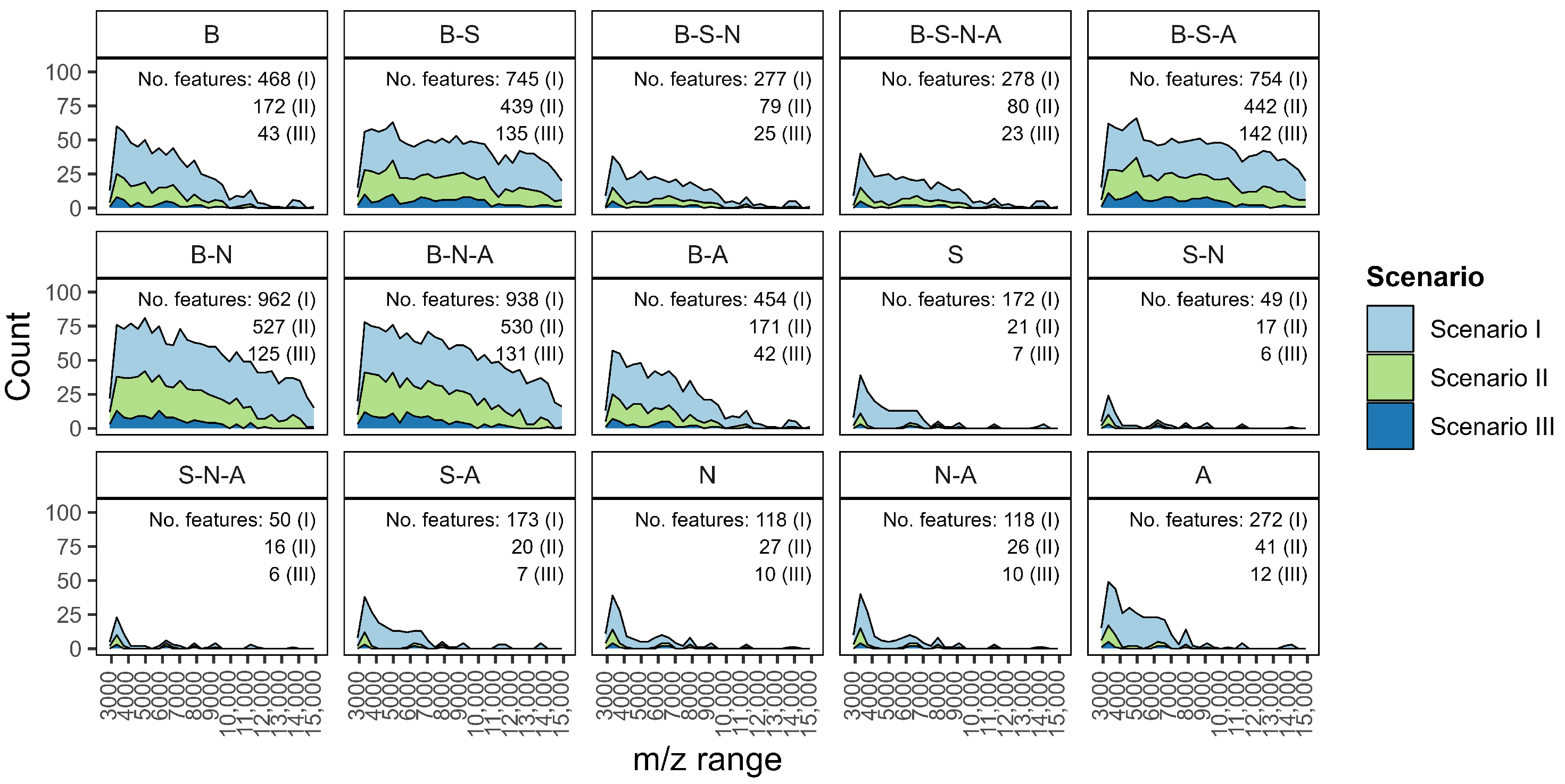
- Pre-processing combinations. Select the pre-processing steps with care, as they directly influence not only the number and nature of extracted features, but also their distribution across the m/z range. For example, combinations beginning with baseline correction tend to preserve features across a wider m/z interval, whereas others may prioritize narrower but potentially more specific spectral zones. Understanding how different combinations behave for your dataset is essential to ensure that relevant biological signals are retained and emphasized in downstream analysis.
- 2.
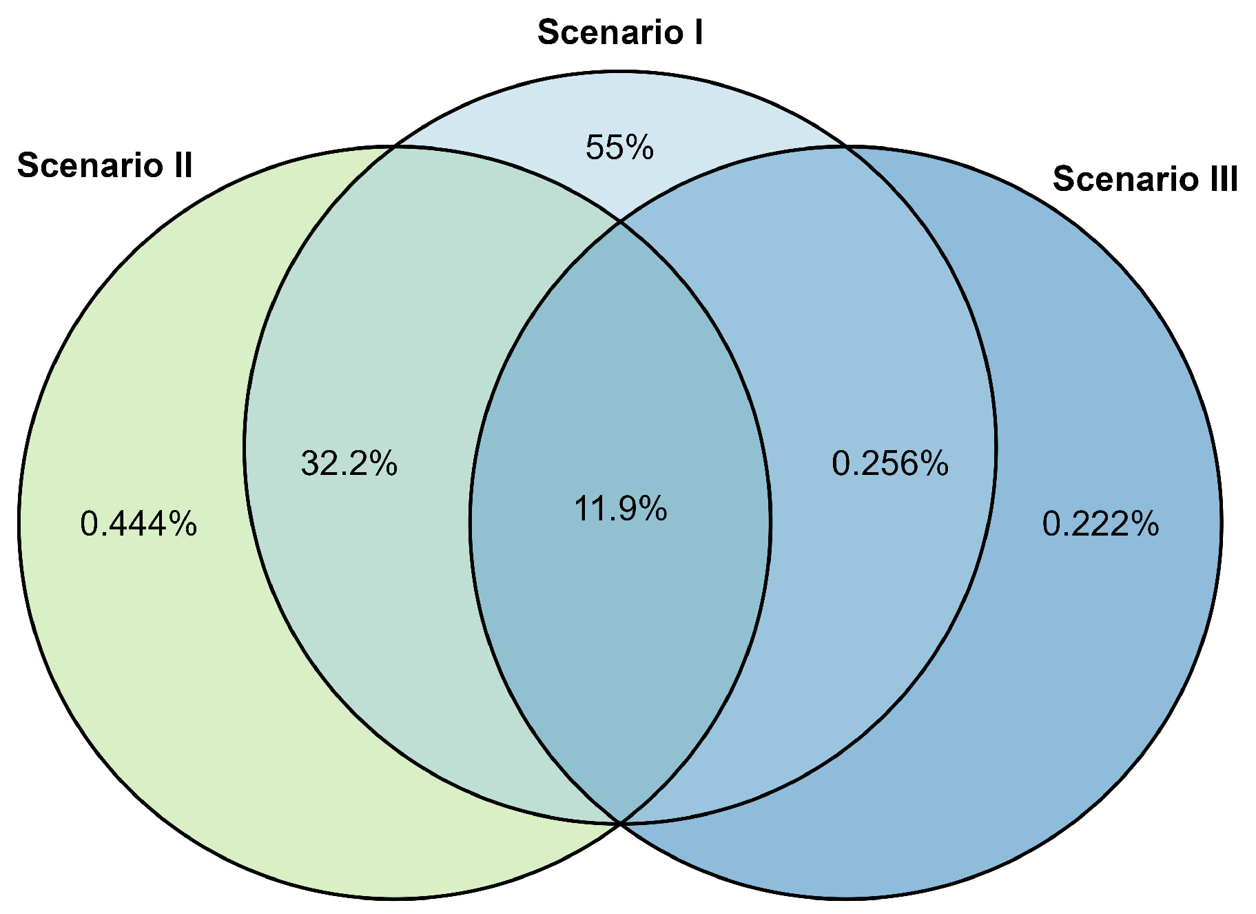
- Intra- and inter-patient filter setting. The filter’s value has an impact on the overall number of extracted features included in the model for signature identification. Low filter levels may better fit with heterogeneous data, while high filter levels may better fit with homogeneous data. Importantly, intra- and inter-patient filtering do not indiscriminately reduce the feature space, but rather reduce unwanted variability: intra-patient filters help control for artifacts and noise within a sample, while inter-patient filters (applied among samples with the same diagnostic label) reduce variability not associated with the disease itself. Nonetheless, excessive filtering can be harmful, especially in heterogeneous cohorts. Therefore, such parameters must be carefully evaluated according to the context. Our results indicate that lower filtering levels often better preserve diagnostically relevant information.
- 3.
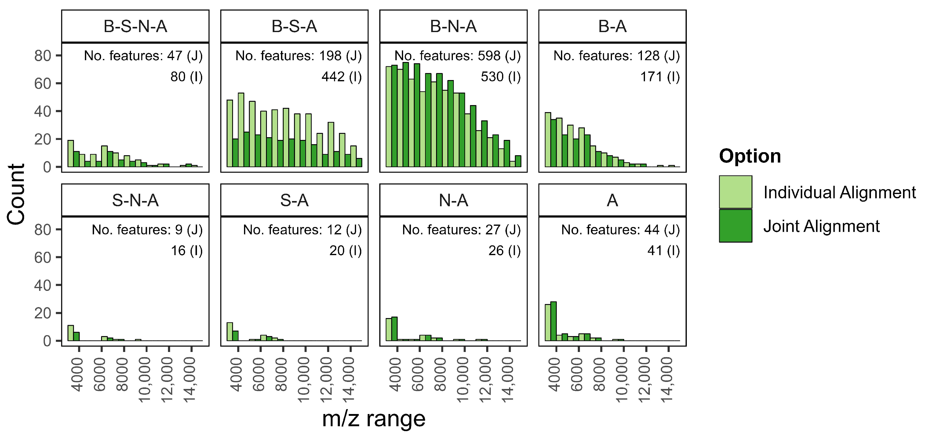
- Individual over joint alignment. Individual alignment is favored as it ensures that the inclusion of new patients in the validation cohort does not retroactively affect the spectra of the training cohort and the associated feature set. This is particularly relevant when aiming for robust and reproducible workflows in prospective studies. In our analysis, individual alignment provided more consistent and reliable feature sets across patients, whereas joint alignment introduced variations that could confound model interpretation and performance.
5. Conclusions
Author Contributions
Funding
Institutional Review Board Statement
Informed Consent Statement
Data Availability Statement
Conflicts of Interest
Abbreviations
| AUC | Area Under Curve |
| FNA | Fine Needle Aspiration |
| HP | Hyperplastic |
| HT | Hashimoto Thyroiditis |
| LASSO | Least Absolute Shrinkage and Selection Operator |
| MALDI | Matrix Assisted Laser Desorption Ionization |
| MSI | Mass Spectrometry Imaging |
| PTC | Papillary Thyroid Carcinoma |
| ROC | Receiver Operating characteristic Curve |
Appendix A. Additional Information, Tables & Figures
Appendix A.1. Computational Resources
Appendix A.2. Figures
Appendix A.3. Tables

| Name | Step | Method | Parameters |
|---|---|---|---|
| B | Baseline | median method | |
| S | Smoothing | moving average | window equal to five |
| N | Normalization | total ion current | |
| A | Alignment | mean absolute deviation | half window width of five |
| P | Peak detection | mean absolute deviation | half window equal to five |
| signal-to-noise ratio equal to six |
| Diagnosis | |||
|---|---|---|---|
| Patient ID | Cellular Composition | Cytological | Histological |
| 1081 | Rich | TIR2 | HT |
| 1082 | Good | TIR3 | HT |
| 1083 | Rich | TIR2 | HT |
| 1084 | Poor | TIR5 | PTC |
| 1084 ex-vivo | Rich | TIR5 | PTC |
| 1123 | Good | TIR2 | Hp |
| 1126 | Poor | TIR5 | PTC |
| 1149 | Good | TIR5 | PTC |
| 1156 | Good | TIR2 | Hp |
| 1187 | Poor | TIR5 | PTC |
| 1188 | Poor | TIR5 | PTC |
| 1188 ex-vivo | Good | TIR5 | PTC |
| 1202 | Rich | TIR4 | PTC |
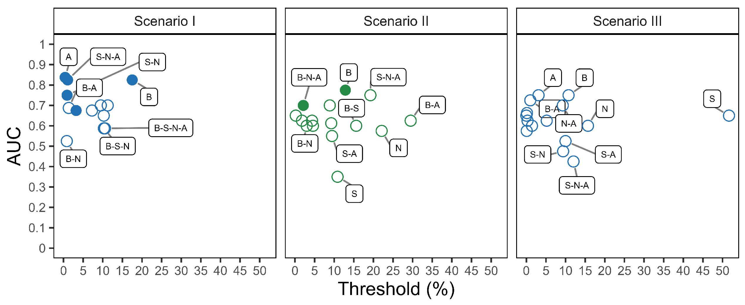
| Classification Performance | ||||
|---|---|---|---|---|
| Combination | AUC | Threshold | Sensitivity | Specificity |
| A | 0.84 (0.60, 1.00) | 0.4% | 0.75 (0.50, 1.00) | 1.00 (1.00, 1.00) |
| B | 0.83 (0.57, 1.00) | 18% | 0.75 (0.50, 1.00) | 1.00 (1.00, 1.00) |
| S-N-A | 0.83 (0.57, 1.00) | 1% | 0.88 (0.63, 1.00) | 0.80 (0.40, 1.00) |
| S-N | 0.75 (0.46, 1.00) | 9% | 0.75 (0.38, 1.00) | 0.80 (0.40, 1.00) |
| S-A | 0.70 (0.39, 1.00) | 10% | 0.50 (0.13, 0.88) | 1.00 (1.00, 1.00) |
| N-A | 0.70 (0.39, 1.00) | 11% | 0.63 (0.25, 0.88) | 1.00 (1.00, 1.00) |
| B-A | 0.69 (0.37, 1.00) | 1% | 0.63 (0.25, 0.88) | 0.80 (0.40, 1.00) |
| B-N-A | 0.68 (0.34, 1.00) | 3% | 0.75 (0.50, 1.00) | 0.80 (0.40, 1.00) |
| S | 0.68 (0.36, 0.99) | 7% | 0.50 (0.13, 0.88) | 1.00 (1.00, 1.00) |
| N | 0.65 (0.32, 0.98) | 10% | 0.63 (0.25, 0.88) | 0.80 (0.40, 1.00) |
| B-S-N | 0.59 (0.25, 0.92) | 10% | 0.50 (0.13, 0.88) | 1.00 (1.00, 1.00) |
| B-S-N-A | 0.59 (0.25, 0.92) | 11% | 0.63 (0.25, 1.00) | 1.00 (1.00, 1.00) |
| B-S | 0.50 (0.50, 0.50) | 0 or 1 | 1 or 0 | |
| B-S-A | 0.50 (0.50, 0.50) | 0 or 1 | 1 or 0 | |
| Classification Performance | ||||
|---|---|---|---|---|
| Combination | AUC | Threshold | Sensitivity | Specificity |
| B | 0.78 (0.48, 1.00) | 13% | 0.75 (0.38, 1.00) | 1.00 (1.00, 1.00) |
| S-N-A | 0.75 (0.46, 1.00) | 19% | 0.50 (0.13, 0.88) | 1.00 (1.00, 1.00) |
| B-S-A | 0.70 (0.38, 1.00) | 9% | 0.63 (0.25, 0.88) | 0.80 (0.40, 1.00) |
| B-N-A | 0.70 (0.37, 1.00) | 2% | 0.75 (0.38, 1.00) | 0.80 (0.40, 1.00) |
| B-S-N | 0.65 (0.36, 0.94) | 0.2% | 0.50 (0.13, 0.88) | 1.00 (1.00, 1.00) |
| B-S-N-A | 0.63 (0.27, 0.98) | 2% | 0.63 (0.25, 1.00) | 1.00 (1.00, 1.00) |
| B-A | 0.63 (0.30, 0.95) | 30% | 0.50 (0.13, 0.88) | 1.00 (1.00, 1.00) |
| A | 0.63 (0.30, 0.95) | 4% | 0.50 (0.13, 0.88) | 1.00 (1.00, 1.00) |
| N-A | 0.61 (0.28, 0.94) | 9% | 0.50 (0.13, 0.88) | 1.00 (1.00, 1.00) |
| B-S | 0.60 (0.26, 0.94) | 16% | 0.63 (0.25, 0.88) | 0.80 (0.40, 1.00) |
| B-N | 0.60 (0.26, 0.94) | 3% | 0.63 (0.25, 1.00) | 0.80 (0.40, 1.00) |
| S-N | 0.60 (0.26, 0.94) | 5% | 0.63 (0.25, 1.00) | 0.80 (0.40, 1.00) |
| N | 0.58 (0.23, 0.92) | 22% | 0.50 (0.13, 0.88) | 1.00 (1.00, 1.00) |
| S-A | 0.55 (0.20, 0.90) | 9% | 0.50 (0.13, 0.88) | 1.00 (1.00, 1.00) |
| S | 0.35 (0.02, 0.68) | 11% | 0.25 (0.00, 0.50) | 1.00 (1.00, 1.00) |
| Classification Performance | ||||
|---|---|---|---|---|
| Combination | AUC | Threshold | Sensitivity | Specificity |
| B | 0.75 (0.48, 1.00) | 11% | 0.50 (0.13, 0.88) | 1.00 (1.00, 1.00) |
| A | 0.75 (0.46, 1.00) | 3% | 0.63 (0.25, 0.88) | 1.00 (1.00, 1.00) |
| B-A | 0.73 (0.43, 1.00) | 1% | 0.63 (0.25, 0.88) | 1.00 (1.00, 1.00) |
| N-A | 0.70 (0.38, 1.00) | 9% | 0.63 (0.25, 0.88) | 1.00 (1.00, 1.00) |
| B-S | 0.63 (0.38, 0.88) | 5% | 0.38 (0.00, 0.75) | 1.00 (1.00, 1.00) |
| B-S-N-A | 0.63 (0.38, 0.87) | 0.3% | 0.38 (0.13, 0.88) | 0.80 (0.40, 1.00) |
| B-S-N | 0.65 (0.38, 0.92) | 0.004% | 0.50 (0.125, 0.875) | 0.80 (0.40, 1.00) |
| B-N | 0.66 (0.34, 0.97) | 0.2% | 0.63 (0.25, 0.88) | 0.80 (0.40, 1.00) |
| S | 0.65 (0.33, 0.97) | 52% | 0.38 (0.00, 0.75) | 1.00 (1.00, 1.00) |
| B-S-A | 0.58 (0.29, 0.86) | 0.09% | 0.38 (0.00, 0.75) | 0.80 (0.40, 1.00) |
| B-N-A | 0.60 (0.27, 0.93) | 1% | 0.50 (0.13, 0.88) | 0.80 (0.40, 1.00) |
| N | 0.60 (0.25, 0.95) | 16 | 0.50% (0.13, 0.88) | 0.80 (0.40, 1.00) |
| S-A | 0.53 (0.19, 0.86) | 0% | 0.38 (0.00, 0.75) | 1.00 (1.00, 1.00) |
| S-N | 0.48 (0.13, 0.82) | 9% | 0.50 (0.13, 0.88) | 0.80 (0.40, 1.00) |
| S-N-A | 0.43 (0.08, 0.77) | 12% | 0.38 (0.13, 0.75) | 1.00 (1.00, 1.00) |
References
- Rohner, T.C.; Staab, D.; Stoeckli, M. MALDI mass spectrometric imaging of biological tissue sections. Mech. Ageing Dev. 2005, 126, 177–185. [Google Scholar] [CrossRef] [PubMed]
- Boggio, K.J.; Obasuyi, E.; Sugino, K.; Nelson, S.B.; Agar, N.Y.; Agar, J.N. Recent advances in single-cell MALDI mass spectrometry imaging and potential clinical impact. Expert. Rev. Proteom. 2011, 8, 591–604. [Google Scholar] [CrossRef] [PubMed]
- Kurczyk, A.; Gawin, M.; Chekan, M.; Wilk, A.; Łakomiec, K.; Mrukwa, G.; Fratczak, K.; Polanska, J.; Fujarewicz, K.; Pietrowska, M.; et al. Classification of thyroid tumors based on mass spectrometry imaging of tissue microarrays; a single-pixel approach. Int. J. Mol. Sci. 2020, 21, 6289. [Google Scholar] [CrossRef]
- Deininger, S.O.; Bollwein, C.; Casadonte, R.; Wandernoth, P.; Gonçalves, J.P.L.; Kriegsmann, K.; Kriegsmann, M.; Boskamp, T.; Kriegsmann, J.; Weichert, W.; et al. Multicenter Evaluation of Tissue Classification by Matrix-Assisted Laser Desorption/Ionization Mass Spectrometry Imaging. Anal. Chem. 2022, 94, 8194–8201. [Google Scholar] [CrossRef]
- He, M.J.; Pu, W.; Wang, X.; Zhang, W.; Donge, T.; Dai, Y. Comparing DESI-MSI and MALDI-MSI mediated spatial metabolomics and their applications in cancer studies. Front. Oncol. 2022, 12, 891018. [Google Scholar] [CrossRef]
- Gonçalves, J.P.L.; Bollwein, C.; Schlitter, A.M.; Kriegsmann, M.; Jacob, A.; Weichert, W.; Schwamborn, K. MALDI-MSI: A Powerful Approach to Understand Primary Pancreatic Ductal Adenocarcinoma and Metastases. Molecules 2022, 27, 4811. [Google Scholar] [CrossRef]
- Capitoli, G.; Piga, I.; L’Imperio, V.; Clerici, F.; Leni, D.; Garancini, M.; Casati, G.; Galimberti, S.; Magni, F.; Pagni, F. Cytomolecular Classification of Thyroid Nodules Using Fine-Needle Washes Aspiration Biopsies. Int. J. Mol. Sci. 2022, 23, 4156. [Google Scholar] [CrossRef]
- Barajas-Solano, C.; Muñoz, B.; Chicano-Gálvez, E.; Escobar, P.; Mejía-Ospino, E. Discriminator for Cutaneous Leishmaniasis Using MALDI-MSI in a Murine Model. J. Am. Soc. Mass Spectrom. 2022, 33, 952–960. [Google Scholar] [CrossRef] [PubMed]
- Gibb, S.; Strimmer, K. MALDIquant: A versatile R package for the analysis of mass spectrometry data. Bioinformatics 2012, 28, 2270–2271. [Google Scholar] [CrossRef]
- Norris, J.L.; Cornett, D.S.; Mobley, J.A.; Andersson, M.; Seeley, E.H.; Chaurand, P.; Caprioli, R.M. Processing MALDI mass spectra to improve mass spectral direct tissue analysis. Int. J. Mass Spectrom. 2007, 260, 212–221. [Google Scholar] [CrossRef]
- Coombes, K.R.; Baggerly, K.A.; Morris, J.S. Pre-processing mass spectrometry data. In Fundamentals of Data Mining in Genomics and Proteomics; Springer: Berlin/Heidelberg, Germany, 2007; pp. 79–102. [Google Scholar]
- Pelikan, R.C.; Hauskrecht, M. Automatic Selection of Preprocessing Methods for Improving Predictions on Mass Spectrometry Protein Profiles. In Proceedings of the AMIA Annual Symposium Proceedings, Washington, DC, USA, 13–17 November 2010; pp. 632–636. [Google Scholar]
- Pérez-Cova, M.; Bedia, C.; Stoll, D.R.; Tauler, R.; Jaumot, J. MSroi: A pre-processing tool for mass spectrometry-based studies. Chemometr. Intell. Lab. 2021, 215, 104333. [Google Scholar] [CrossRef]
- Ozcift, A.; Gulten, A. Assessing effects of pre-processing mass spectrometry data on classification performance. Eur. J. Mass Spectrom. 2008, 14, 267–273. [Google Scholar] [CrossRef] [PubMed]
- Cruz-Marcelo, A.; Guerra, R.; Vannucci, M.; Li, Y.; Lau, C.C.; Man, T.K. Comparison of algorithms for pre-processing of SELDI-TOF mass spectrometry data. Bioinformatics 2008, 24, 2129–2136. [Google Scholar] [CrossRef] [PubMed]
- Emanuele, V.A.; Gurbaxani, B.M. Benchmarking currently available SELDI-TOF MS preprocessing techniques. Proteomics 2009, 9, 1754–1762. [Google Scholar] [CrossRef] [PubMed]
- Abdelmoula, W.M.; Lopez, B.G.C.; Randall, E.C.; Kapur, T.; Sarkaria, J.N.; White, F.M.; Agar, J.N.; Wells, W.M.; Agar, N.Y. Peak learning of mass spectrometry imaging data using artificial neural networks. Nat. Commun. 2021, 12, 5544. [Google Scholar] [CrossRef]
- Lieb, F.; Boskamp, T.; Stark, H.G. Peak detection for MALDI mass spectrometry imaging data using sparse frame multipliers. J. Proteom. 2020, 225, 103852. [Google Scholar] [CrossRef]
- Cleary, J.L.; Luu, G.T.; Pierce, E.C.; Dutton, R.J.; Sanchez, L.M. BLANKA: An Algorithm for blank subtraction in mass spectrometry of complex biological samples. J. Am. Soc. Mass Spectrom. 2019, 30, 1426–1434. [Google Scholar] [CrossRef]
- Wegdam, W.; Moerland, P.D.; Buist, M.R.; van Themaat, E.; Bleijlevens, B.; Hoefsloot, H.C.; de Koster, C.G.; Aerts, J.M. Classification-based comparison of pre-processing methods for interpretation of mass spectrometry generated clinical datasets. Proteome Sci. 2009, 7, 19. [Google Scholar] [CrossRef] [PubMed]
- Oliveira, C.; Longuespée, R. MALDImID: Spatialomics R package and Shiny app for more specific identification of MALDI imaging proteolytic peaks using LC-MS/MS-based proteomic biomarker discovery data. Proteomics 2023, 23, 2300005. [Google Scholar] [CrossRef]
- Robichaud, G.; Garrard, K.P.; Barry, J.A.; Muddiman, D.C. MSiReader: An open-source interface to view and analyze high resolving power MS imaging files on Matlab platform. J. Am. Soc. Mass Spectrom. 2013, 24, 718–721. [Google Scholar] [CrossRef]
- Jagadeesan, K.K.; Ekström, S. MALDIViz: A comprehensive informatics tool for MALDI-MS data visualization and analysis. Slas Discov. Adv. Life Sci. R&D 2017, 22, 1246–1252. [Google Scholar]
- Bemis, K.A.; Föll, M.C.; Guo, D.; Lakkimsetty, S.S.; Vitek, O. Cardinal v. 3: A versatile open-source software for mass spectrometry imaging analysis. Nat. Methods 2023, 20, 1883–1886. [Google Scholar] [CrossRef] [PubMed]
- Romano, P.; Profumo, A.; Facchiano, A. Pre-Processing MALDI/TOF Mass Spectra by Using Geena 2. Curr. Protoc. Bioinform. 2018, 64, e59. [Google Scholar] [CrossRef] [PubMed]
- Capitoli, G.; Piga, I.; Clerici, F.; Brambilla, V.; Mahajneh, A.; Leni, D.; Garancini, M.; Pincelli, A.I.; L’Imperio, V.; Galimberti, S.; et al. Analysis of Hashimoto’s thyroiditis on fine needle aspiration samples by MALDI-Imaging. BBA-Proteins Proteom. 2020, 1868, 140481. [Google Scholar] [CrossRef]

| Combination | Baseline | Smoothing | Normalization | Alignment | Peak Detection |
|---|---|---|---|---|---|
| B | X | X | |||
| B-S | X | X | X | ||
| B-S-N | X | X | X | X | |
| B-S-N-A | X | X | X | X | X |
| B-S-A | X | X | X | X | |
| B-N | X | X | X | ||
| B-N-A | X | X | X | X | |
| B-A | X | X | X | ||
| S | X | X | |||
| S-N | X | X | X | ||
| S-N-A | X | X | X | X | |
| S-A | X | X | X | ||
| N | X | X | |||
| N-A | X | X | X | ||
| A | X | X |
Disclaimer/Publisher’s Note: The statements, opinions and data contained in all publications are solely those of the individual author(s) and contributor(s) and not of MDPI and/or the editor(s). MDPI and/or the editor(s) disclaim responsibility for any injury to people or property resulting from any ideas, methods, instructions or products referred to in the content. |
© 2025 by the authors. Licensee MDPI, Basel, Switzerland. This article is an open access article distributed under the terms and conditions of the Creative Commons Attribution (CC BY) license (https://creativecommons.org/licenses/by/4.0/).
Share and Cite
Capitoli, G.; van Abeelen, K.C.J.; Piga, I.; L’Imperio, V.; Nobile, M.S.; Besozzi, D.; Galimberti, S. Well Begun Is Half Done: The Impact of Pre-Processing in MALDI Mass Spectrometry Imaging Analysis Applied to a Case Study of Thyroid Nodules. Stats 2025, 8, 57. https://doi.org/10.3390/stats8030057
Capitoli G, van Abeelen KCJ, Piga I, L’Imperio V, Nobile MS, Besozzi D, Galimberti S. Well Begun Is Half Done: The Impact of Pre-Processing in MALDI Mass Spectrometry Imaging Analysis Applied to a Case Study of Thyroid Nodules. Stats. 2025; 8(3):57. https://doi.org/10.3390/stats8030057
Chicago/Turabian StyleCapitoli, Giulia, Kirsten C. J. van Abeelen, Isabella Piga, Vincenzo L’Imperio, Marco S. Nobile, Daniela Besozzi, and Stefania Galimberti. 2025. "Well Begun Is Half Done: The Impact of Pre-Processing in MALDI Mass Spectrometry Imaging Analysis Applied to a Case Study of Thyroid Nodules" Stats 8, no. 3: 57. https://doi.org/10.3390/stats8030057
APA StyleCapitoli, G., van Abeelen, K. C. J., Piga, I., L’Imperio, V., Nobile, M. S., Besozzi, D., & Galimberti, S. (2025). Well Begun Is Half Done: The Impact of Pre-Processing in MALDI Mass Spectrometry Imaging Analysis Applied to a Case Study of Thyroid Nodules. Stats, 8(3), 57. https://doi.org/10.3390/stats8030057