
Comparing Robust Haberman Linking and Invariance Alignment


Abstract
1. Introduction
2. Unidimensional Factor Model
2.1. Dichotomous Items
2.2. Continuous Items
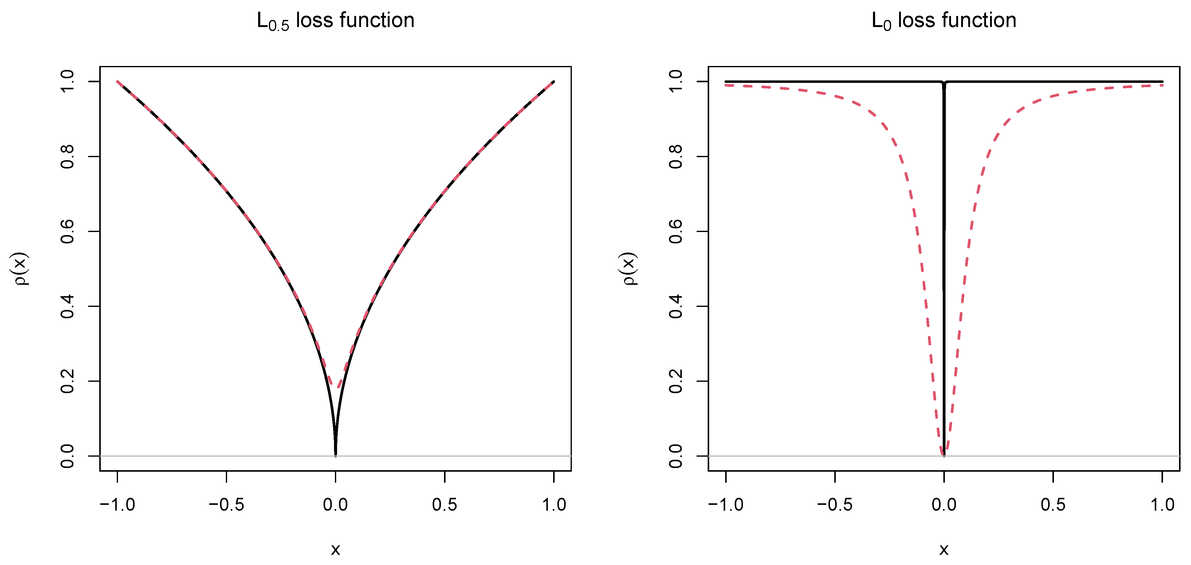
3. and Loss Functions
4. Invariance Alignment
5. Haberman Linking
6. Simulation Study 1: Dichotomous Items
6.1. Method
6.2. Results
7. Simulation Study 2: Continuous Items
7.1. Method
7.2. Results
8. Discussion
Funding
Institutional Review Board Statement
Informed Consent Statement
Data Availability Statement
Conflicts of Interest
Abbreviations
| 2PL | Two-parameter logistic |
| CFA | Confirmatory factor analysis |
| DIF | Differential item functioning |
| HL | Haberman linking |
| IA | Invariance alignment |
| IRF | Item response function |
| IRT | Item response theory |
| MML | Marginal maximum likelihood |
| RMSE | Root mean square error |
| SD | Standard deviation |
References
- Bartholomew, D.J.; Knott, M.; Moustaki, I. Latent Variable Models and Factor Analysis: A Unified Approach; Wiley: New York, NY, USA, 2011. [Google Scholar] [CrossRef]
- Bock, R.D.; Gibbons, R.D. Item Response Theory; Wiley: Hoboken, NJ, USA, 2021. [Google Scholar] [CrossRef]
- Chen, Y.; Li, X.; Liu, J.; Ying, Z. Item response theory—A statistical framework for educational and psychological measurement. arXiv 2021, arXiv:2108.08604. [Google Scholar] [CrossRef]
- Meredith, W. Measurement invariance, factor analysis and factorial invariance. Psychometrika 1993, 58, 525–543. [Google Scholar] [CrossRef]
- Millsap, R.E. Statistical Approaches to Measurement Invariance; Routledge: New York, NY, USA, 2011. [Google Scholar] [CrossRef]
- Mellenbergh, G.J. Item bias and item response theory. Int. J. Educ. Res. 1989, 13, 127–143. [Google Scholar] [CrossRef]
- Bauer, D.J. Enhancing measurement validity in diverse populations: Modern approaches to evaluating differential item functioning. Brit. J. Math. Stat. Psychol. 2023, 76, 435–461. [Google Scholar] [CrossRef]
- Holland, P.W.; Wainer, H. (Eds.) Differential Item Functioning: Theory and Practice; Lawrence Erlbaum: Hillsdale, NJ, USA, 1993. [Google Scholar] [CrossRef]
- Penfield, R.D.; Camilli, G. Differential item functioning and item bias. In Handbook of Statistics; Volume 26: Psychometrics; Rao, C.R., Sinharay, S., Eds.; Elsevier: Amsterdam, The Netherlands, 2007; pp. 125–167. [Google Scholar] [CrossRef]
- Thissen, D. A review of some of the history of factorial invariance and differential item functioning. Multivar. Behav. Res. 2024. epub ahead of print. [Google Scholar] [CrossRef]
- Wells, C.S. Assessing Measurement Invariance for Applied Research; Cambridge University Press: Cambridge, UK, 2021. [Google Scholar] [CrossRef]
- Asparouhov, T.; Muthén, B. Multiple-group factor analysis alignment. Struct. Equ. Model. 2014, 21, 495–508. [Google Scholar] [CrossRef]
- Asparouhov, T.; Muthén, B. Penalized structural equation models. Struct. Equ. Model. 2024, 31, 429–454. [Google Scholar] [CrossRef]
- Muthén, B.; Asparouhov, T. IRT studies of many groups: The alignment method. Front. Psychol. 2014, 5, 978. [Google Scholar] [CrossRef] [PubMed]
- Muthén, B.; Asparouhov, T. Recent methods for the study of measurement invariance with many groups: Alignment and random effects. Sociol. Methods Res. 2018, 47, 637–664. [Google Scholar] [CrossRef]
- Cieciuch, J.; Davidov, E.; Schmidt, P. Alignment optimization. Estimation of the most trustworthy means in cross-cultural studies even in the presence of noninvariance. In Cross-Cultural Analysis: Methods and Applications; Davidov, E., Schmidt, P., Billiet, J., Eds.; Routledge: Oxfordshire, UK, 2018; pp. 571–592. [Google Scholar] [CrossRef]
- Pokropek, A.; Davidov, E.; Schmidt, P. A Monte Carlo simulation study to assess the appropriateness of traditional and newer approaches to test for measurement invariance. Struct. Equ. Model. 2019, 26, 724–744. [Google Scholar] [CrossRef]
- Fischer, R.; Karl, J.A. A primer to (cross-cultural) multi-group invariance testing possibilities in R. Front. Psychol. 2019, 10, 1507. [Google Scholar] [CrossRef]
- Han, H. Using measurement alignment in research on adolescence involving multiple groups: A brief tutorial with R. J. Res. Adolesc. 2024, 34, 235–242. [Google Scholar] [CrossRef]
- Lai, M.H.C. Adjusting for measurement noninvariance with alignment in growth modeling. Multivar. Behav. Res. 2023, 58, 30–47. [Google Scholar] [CrossRef] [PubMed]
- Leitgöb, H.; Seddig, D.; Asparouhov, T.; Behr, D.; Davidov, E.; De Roover, K.; Jak, S.; Meitinger, K.; Menold, N.; Muthén, B.; et al. Measurement invariance in the social sciences: Historical development, methodological challenges, state of the art, and future perspectives. Soc. Sci. Res. 2023, 110, 102805. [Google Scholar] [CrossRef]
- Luong, R.; Flake, J.K. Measurement invariance testing using confirmatory factor analysis and alignment optimization: A tutorial for transparent analysis planning and reporting. Psychol. Methods 2023, 28, 905–924. [Google Scholar] [CrossRef] [PubMed]
- Sideridis, G.; Alghamdi, M.H. Bullying in middle school: Evidence for a multidimensional structure and measurement invariance across gender. Children 2023, 10, 873. [Google Scholar] [CrossRef]
- Tsaousis, I.; Jaffari, F.M. Identifying bias in social and health research: Measurement invariance and latent mean differences using the alignment approach. Mathematics 2023, 11, 4007. [Google Scholar] [CrossRef]
- Wurster, S. Measurement invariance of non-cognitive measures in TIMSS across countries and across time. An application and comparison of multigroup confirmatory factor analysis, Bayesian approximate measurement invariance and alignment optimization approach. Stud. Educ. Eval. 2022, 73, 101143. [Google Scholar] [CrossRef]
- Haberman, S.J. Linking Parameter Estimates Derived from an Item Response Model Through Separate Calibrations; (Research Report No. RR-09-40); Educational Testing Service: Princeton, NJ, USA, 2009. [Google Scholar] [CrossRef]
- Kolen, M.J.; Brennan, R.L. Test Equating, Scaling, and Linking; Springer: New York, NY, USA, 2014. [Google Scholar] [CrossRef]
- Lee, W.C.; Lee, G. IRT linking and equating. In The Wiley Handbook of Psychometric Testing: A Multidisciplinary Reference on Survey, Scale and Test; Irwing, P., Booth, T., Hughes, D.J., Eds.; Wiley: New York, NY, USA, 2018; pp. 639–673. [Google Scholar] [CrossRef]
- Sansivieri, V.; Wiberg, M.; Matteucci, M. A review of test equating methods with a special focus on IRT-based approaches. Statistica 2017, 77, 329–352. [Google Scholar] [CrossRef]
- Höft, L.; Bernholt, S. Longitudinal couplings between interest and conceptual understanding in secondary school chemistry: An activity-based perspective. Int. J. Sci. Educ. 2019, 41, 607–627. [Google Scholar] [CrossRef]
- Liu, G.; Kim, H.J.; Lee, W.C.; Kim, Y. Comparison of Simultaneous Linking and Separate Calibration with Stocking-Lord Method; (CASMA Research Report Number 57); Center for Advanced Studies in Measurement and Assessment, University of Iowa: Iowa City, IA, USA, 2024; Available online: https://tinyurl.com/2bj6pbwn (accessed on 20 December 2024).
- Moehring, A.; Schroeders, U.; Wilhelm, O. Knowledge is power for medical assistants: Crystallized and fluid intelligence as predictors of vocational knowledge. Front. Psychol. 2018, 9, 28. [Google Scholar] [CrossRef]
- Neuenschwander, M.P.; Mayland, C.; Niederbacher, E.; Garrote, A. Modifying biased teacher expectations in mathematics and German: A teacher intervention study. Learn. Individ. Differ. 2021, 87, 101995. [Google Scholar] [CrossRef]
- Sewasew, D.; Schroeders, U.; Schiefer, I.M.; Weirich, S.; Artelt, C. Development of sex differences in math achievement, self-concept, and interest from grade 5 to 7. Contemp. Educ. Psychol. 2018, 54, 55–65. [Google Scholar] [CrossRef]
- Avvisati, F.; Le Donné, N.; Paccagnella, M. A meeting report: Cross-cultural comparability of questionnaire measures in large-scale international surveys. Meas. Instrum. Soc. Sci. 2019, 1, 8. [Google Scholar] [CrossRef]
- Robitzsch, A. Lp loss functions in invariance alignment and Haberman linking with few or many groups. Stats 2020, 3, 246–283. [Google Scholar] [CrossRef]
- Birnbaum, A. Some latent trait models and their use in inferring an examinee’s ability. In Statistical Theories of Mental Test Scores; Lord, F.M., Novick, M.R., Eds.; MIT Press: Reading, MA, USA, 1968; pp. 397–479. [Google Scholar]
- Aitkin, M. Expectation maximization algorithm and extensions. In Handbook of Item Response Theory, Volume 2: Statistical Tools; van der Linden, W.J., Ed.; CRC Press: Boca Raton, FL, USA, 2016; pp. 217–236. [Google Scholar] [CrossRef]
- Bock, R.D.; Aitkin, M. Marginal maximum likelihood estimation of item parameters: Application of an EM algorithm. Psychometrika 1981, 46, 443–459. [Google Scholar] [CrossRef]
- Glas, C.A.W. Maximum-likelihood estimation. In Handbook of Item Response Theory, Volume 2: Statistical Tools; van der Linden, W.J., Ed.; CRC Press: Boca Raton, FL, USA, 2016; pp. 197–216. [Google Scholar] [CrossRef]
- Basilevsky, A.T. Statistical Factor Analysis and Related Methods: Theory and Applications; Wiley: New York, NY, USA, 2009. [Google Scholar] [CrossRef]
- De Boeck, P. Random item IRT models. Psychometrika 2008, 73, 533–559. [Google Scholar] [CrossRef]
- Halpin, P.F. Differential item functioning via robust scaling. Psychometrika 2024, 89, 796–821. [Google Scholar] [CrossRef] [PubMed]
- Magis, D.; De Boeck, P. Identification of differential item functioning in multiple-group settings: A multivariate outlier detection approach. Multivar. Behav. Res. 2011, 46, 733–755. [Google Scholar] [CrossRef] [PubMed]
- Robitzsch, A. Robust and nonrobust linking of two groups for the Rasch model with balanced and unbalanced random DIF: A comparative simulation study and the simultaneous assessment of standard errors and linking errors with resampling techniques. Symmetry 2021, 13, 2198. [Google Scholar] [CrossRef]
- Robitzsch, A. Comparing robust linking and regularized estimation for linking two groups in the 1PL and 2PL models in the presence of sparse uniform differential item functioning. Stats 2023, 6, 192–208. [Google Scholar] [CrossRef]
- Tutz, G.; Schauberger, G. A penalty approach to differential item functioning in Rasch models. Psychometrika 2015, 80, 21–43. [Google Scholar] [CrossRef] [PubMed]
- Wang, W.; Liu, Y.; Liu, H. Testing differential item functioning without predefined anchor items using robust regression. J. Educ. Behav. Stat. 2022, 47, 666–692. [Google Scholar] [CrossRef]
- Huber, P.J.; Ronchetti, E.M. Robust Statistics; Wiley: New York, NY, USA, 2009. [Google Scholar] [CrossRef]
- Maronna, R.A.; Martin, R.D.; Yohai, V.J. Robust Statistics: Theory and Methods; Wiley: New York, NY, USA, 2006. [Google Scholar] [CrossRef]
- Wilcox, R.R.; Keselman, H.J. Modern robust data analysis methods: Measures of central tendency. Psychol. Methods 2003, 8, 254–274. [Google Scholar] [CrossRef]
- Giacalone, M.; Panarello, D.; Mattera, R. Multicollinearity in regression: An efficiency comparison between Lp-norm and least squares estimators. Qual. Quant. 2018, 52, 1831–1859. [Google Scholar] [CrossRef]
- Lipovetsky, S. Optimal Lp-metric for minimizing powered deviations in regression. J. Mod. Appl. Stat. Methods 2007, 6, 20. [Google Scholar] [CrossRef]
- Livadiotis, G. General fitting methods based on Lq norms and their optimization. Stats 2020, 3, 16–31. [Google Scholar] [CrossRef]
- Sposito, V.A. On unbiased Lp regression estimators. J. Am. Stat. Assoc. 1982, 77, 652–653. [Google Scholar]
- Koenker, R.; Hallock, K.F. Quantile regression. J. Econ. Perspect. 2001, 15, 143–156. [Google Scholar] [CrossRef]
- Koenker, R. Quantile regression: 40 years on. Annu. Rev. Econ. 2017, 9, 155–176. [Google Scholar] [CrossRef]
- Robitzsch, A. Implementation aspects in regularized structural equation models. Algorithms 2023, 16, 446. [Google Scholar] [CrossRef]
- Oelker, M.R.; Pößnecker, W.; Tutz, G. Selection and fusion of categorical predictors with L0-type penalties. Stat. Model. 2015, 15, 389–410. [Google Scholar] [CrossRef]
- Oelker, M.R.; Tutz, G. A uniform framework for the combination of penalties in generalized structured models. Adv. Data Anal. Classif. 2017, 11, 97–120. [Google Scholar] [CrossRef]
- O’Neill, M.; Burke, K. Variable selection using a smooth information criterion for distributional regression models. Stat. Comput. 2023, 33, 71. [Google Scholar] [CrossRef] [PubMed]
- Robitzsch, A. L0 and Lp loss functions in model-robust estimation of structural equation models. Psych 2023, 5, 1122–1139. [Google Scholar] [CrossRef]
- Robitzsch, A. Examining differences of invariance alignment in the Mplus software and the R package sirt. Mathematics 2024, 12, 770. [Google Scholar] [CrossRef]
- Mansolf, M.; Vreeker, A.; Reise, S.P.; Freimer, N.B.; Glahn, D.C.; Gur, R.E.; Moore, T.M.; Pato, C.N.; Pato, M.T.; Palotie, A.; et al. Extensions of multiple-group item response theory alignment: Application to psychiatric phenotypes in an international genomics consortium. Educ. Psychol. Meas. 2020, 80, 870–909. [Google Scholar] [CrossRef]
- Muthén, L.; Muthén, B. Mplus User’s Guide, Version 8.11; Muthén & Muthén: Los Angeles, CA, USA, 2024. Available online: https://www.statmodel.com/ (accessed on 22 November 2024).
- Robitzsch, A. Implementation aspects in invariance alignment. Stats 2023, 6, 1160–1178. [Google Scholar] [CrossRef]
- Lietz, P.; Cresswell, J.C.; Rust, K.F.; Adams, R.J. (Eds.) Implementation of Large-Scale Education Assessments; Wiley: New York, NY, USA, 2017. [Google Scholar] [CrossRef]
- Rutkowski, L.; von Davier, M.; Rutkowski, D. (Eds.) A Handbook of International Large-scale Assessment: Background, Technical Issues, and Methods of Data Analysis; Chapman Hall/CRC Press: London, UK, 2013. [Google Scholar] [CrossRef]
- R Core Team. R: A Language and Environment for Statistical Computing; R Core Team: Vienna, Austria, 2024; Available online: https://www.R-project.org (accessed on 15 June 2024).
- Robitzsch, A. sirt: Supplementary Item Response Theory Models, 2024. R Package Version 4.2-89. Available online: https://github.com/alexanderrobitzsch/sirt (accessed on 13 November 2024).
- Rasch, G. Probabilistic Models for Some Intelligence and Attainment Tests; Danish Institute for Educational Research: Copenhagen, Denmark, 1960. [Google Scholar]
- Raykov, T.; Marcoulides, G.A. Introduction to Psychometric Theory; Routledge: London, UK, 2011. [Google Scholar] [CrossRef]
- Monseur, C.; Berezner, A. The computation of equating errors in international surveys in education. J. Appl. Meas. 2007, 8, 323–335. Available online: https://bit.ly/2WDPeqD (accessed on 22 November 2024).
- Camilli, G. The case against item bias detection techniques based on internal criteria: Do item bias procedures obscure test fairness issues? In Differential Item Functioning: Theory and Practice; Holland, P.W., Wainer, H., Eds.; Erlbaum: Hillsdale, NJ, USA, 1993; pp. 397–417. [Google Scholar]
- Funder, D.C.; Gardiner, G. MIsgivings about measurement invariance. Eur. J. Pers. 2024, 38, 889–895. [Google Scholar] [CrossRef]
- Robitzsch, A.; Lüdtke, O. Why full, partial, or approximate measurement invariance are not a prerequisite for meaningful and valid group comparisons. Struct. Equ. Model. 2023, 30, 859–870. [Google Scholar] [CrossRef]
- Shealy, R.; Stout, W. A model-based standardization approach that separates true bias/DIF from group ability differences and detects test bias/DTF as well as item bias/DIF. Psychometrika 1993, 58, 159–194. [Google Scholar] [CrossRef]
- Welzel, C.; Inglehart, R.F. Misconceptions of measurement equivalence: Time for a paradigm shift. Comp. Political Stud. 2016, 49, 1068–1094. [Google Scholar] [CrossRef]
- Fischer, R.; Rudnev, M. From MIsgivings to MIse-en-scène: The role of invariance in personality science. Eur. J. Pers. 2024. epub ahead of print. [Google Scholar] [CrossRef]
- Meuleman, B.; Żółtak, T.; Pokropek, A.; Davidov, E.; Muthén, B.; Oberski, D.L.; Billiet, J.; Schmidt, P. Why measurement invariance is important in comparative research. A response to Welzel et al. (2021). Sociol. Methods Res. 2023, 52, 1401–1419. [Google Scholar] [CrossRef]

| Average Absolute Bias | Average Relative RMSE | |||||||||||||||||
|---|---|---|---|---|---|---|---|---|---|---|---|---|---|---|---|---|---|---|
| IA1 | IA2 | HL1 | HL2 | IA1 | IA2 | HL1 | HL2 | IA1 ‡ | IA2 | HL1 | HL2 | IA1 | IA2 | HL1 | HL2 | |||
| 0 | 10 | 250 | 0.02 | 0.02 | 0.00 | 0.02 | 0.02 | 0.02 | 0.00 | 0.02 | 100 | 101 | 114 | 102 | 122 | 121 | 140 | 123 |
| 500 | 0.01 | 0.02 | 0.00 | 0.02 | 0.01 | 0.01 | 0.00 | 0.01 | 100 | 101 | 113 | 101 | 118 | 119 | 136 | 118 | ||
| 1000 | 0.00 | 0.00 | 0.00 | 0.00 | 0.00 | 0.00 | 0.00 | 0.00 | 100 | 100 | 111 | 100 | 114 | 115 | 128 | 113 | ||
| 2000 | 0.00 | 0.00 | 0.00 | 0.00 | 0.00 | 0.00 | 0.00 | 0.00 | 100 | 100 | 108 | 99 | 108 | 108 | 118 | 106 | ||
| 20 | 250 | 0.01 | 0.02 | 0.00 | 0.02 | 0.01 | 0.01 | 0.00 | 0.01 | 100 | 100 | 110 | 101 | 123 | 123 | 137 | 121 | |
| 500 | 0.01 | 0.01 | 0.00 | 0.01 | 0.01 | 0.01 | 0.00 | 0.01 | 100 | 100 | 109 | 100 | 117 | 117 | 130 | 117 | ||
| 1000 | 0.00 | 0.00 | 0.00 | 0.00 | 0.00 | 0.00 | 0.00 | 0.00 | 100 | 100 | 108 | 100 | 111 | 111 | 122 | 110 | ||
| 2000 | 0.00 | 0.00 | 0.00 | 0.00 | 0.00 | 0.00 | 0.00 | 0.00 | 100 | 100 | 105 | 99 | 104 | 104 | 110 | 102 | ||
| 0.3 | 10 | 250 | 0.07 | 0.07 | 0.06 | 0.07 | 0.06 | 0.06 | 0.07 | 0.06 | 100 | 101 | 117 | 102 | 121 | 122 | 146 | 121 |
| 500 | 0.06 | 0.06 | 0.06 | 0.06 | 0.06 | 0.06 | 0.06 | 0.06 | 100 | 101 | 115 | 101 | 121 | 121 | 144 | 119 | ||
| 1000 | 0.05 | 0.05 | 0.06 | 0.05 | 0.04 | 0.05 | 0.06 | 0.04 | 100 | 101 | 117 | 100 | 120 | 121 | 145 | 118 | ||
| 2000 | 0.03 | 0.03 | 0.04 | 0.03 | 0.02 | 0.02 | 0.04 | 0.02 | 100 | 100 | 128 | 98 | 112 | 112 | 158 | 108 | ||
| 20 | 250 | 0.07 | 0.07 | 0.06 | 0.07 | 0.06 | 0.06 | 0.07 | 0.06 | 100 | 101 | 112 | 101 | 121 | 121 | 141 | 121 | |
| 500 | 0.06 | 0.06 | 0.06 | 0.06 | 0.06 | 0.06 | 0.06 | 0.05 | 100 | 100 | 110 | 101 | 122 | 122 | 139 | 121 | ||
| 1000 | 0.05 | 0.05 | 0.06 | 0.05 | 0.04 | 0.04 | 0.05 | 0.03 | 100 | 100 | 114 | 99 | 116 | 116 | 141 | 111 | ||
| 2000 | 0.03 | 0.03 | 0.04 | 0.03 | 0.01 | 0.01 | 0.03 | 0.01 | 100 | 100 | 123 | 97 | 97 | 97 | 140 | 92 | ||
| 0.6 | 10 | 250 | 0.10 | 0.10 | 0.11 | 0.10 | 0.08 | 0.08 | 0.10 | 0.08 | 100 | 101 | 120 | 100 | 121 | 122 | 152 | 120 |
| 500 | 0.06 | 0.06 | 0.08 | 0.06 | 0.03 | 0.03 | 0.07 | 0.03 | 100 | 100 | 129 | 100 | 118 | 119 | 164 | 115 | ||
| 1000 | 0.03 | 0.03 | 0.05 | 0.03 | 0.00 | 0.00 | 0.03 | 0.00 | 100 | 100 | 132 | 96 | 108 | 107 | 163 | 101 | ||
| 2000 | 0.02 | 0.02 | 0.02 | 0.02 | 0.00 | 0.00 | 0.00 | 0.00 | 100 | 100 | 122 | 95 | 101 | 101 | 128 | 95 | ||
| 20 | 250 | 0.09 | 0.09 | 0.10 | 0.09 | 0.07 | 0.07 | 0.10 | 0.06 | 100 | 100 | 117 | 101 | 120 | 120 | 150 | 119 | |
| 500 | 0.06 | 0.06 | 0.07 | 0.05 | 0.02 | 0.02 | 0.05 | 0.02 | 100 | 100 | 121 | 98 | 108 | 108 | 147 | 105 | ||
| 1000 | 0.03 | 0.03 | 0.04 | 0.03 | 0.00 | 0.00 | 0.01 | 0.00 | 100 | 100 | 120 | 96 | 101 | 101 | 125 | 97 | ||
| 2000 | 0.02 | 0.02 | 0.02 | 0.02 | 0.00 | 0.00 | 0.00 | 0.00 | 100 | 100 | 111 | 96 | 96 | 97 | 105 | 92 | ||
| Average Absolute Bias | Average Relative RMSE | |||||||||||||||||
|---|---|---|---|---|---|---|---|---|---|---|---|---|---|---|---|---|---|---|
| IA1 | IA2 | HL1 | HL2 | IA1 | IA2 | HL1 | HL2 | IA1 ‡ | IA2 | HL1 | HL2 | IA1 | IA2 | HL1 | HL2 | |||
| 0 | 10 | 250 | 0.01 | 0.01 | 0.01 | 0.01 | 0.02 | 0.02 | 0.02 | 0.02 | 100 | 103 | 104 | 104 | 131 | 133 | 135 | 135 |
| 500 | 0.01 | 0.00 | 0.00 | 0.00 | 0.01 | 0.01 | 0.01 | 0.01 | 100 | 102 | 103 | 103 | 129 | 130 | 129 | 129 | ||
| 1000 | 0.00 | 0.00 | 0.00 | 0.00 | 0.01 | 0.01 | 0.01 | 0.01 | 100 | 101 | 101 | 101 | 126 | 126 | 125 | 125 | ||
| 2000 | 0.00 | 0.00 | 0.00 | 0.00 | 0.00 | 0.00 | 0.00 | 0.00 | 100 | 100 | 99 | 99 | 118 | 118 | 116 | 116 | ||
| 20 | 250 | 0.01 | 0.00 | 0.01 | 0.01 | 0.01 | 0.01 | 0.01 | 0.01 | 100 | 101 | 104 | 104 | 136 | 137 | 137 | 137 | |
| 500 | 0.00 | 0.00 | 0.00 | 0.00 | 0.01 | 0.01 | 0.00 | 0.00 | 100 | 101 | 102 | 102 | 131 | 131 | 130 | 130 | ||
| 1000 | 0.00 | 0.00 | 0.00 | 0.00 | 0.00 | 0.00 | 0.00 | 0.00 | 100 | 100 | 101 | 101 | 122 | 122 | 121 | 121 | ||
| 2000 | 0.00 | 0.00 | 0.00 | 0.00 | 0.00 | 0.00 | 0.00 | 0.00 | 100 | 100 | 99 | 99 | 111 | 112 | 109 | 109 | ||
| 0.3 | 10 | 250 | 0.02 | 0.01 | 0.01 | 0.01 | 0.02 | 0.02 | 0.02 | 0.02 | 100 | 103 | 104 | 104 | 133 | 134 | 137 | 137 |
| 500 | 0.01 | 0.01 | 0.01 | 0.01 | 0.01 | 0.01 | 0.01 | 0.01 | 100 | 102 | 103 | 103 | 130 | 131 | 130 | 130 | ||
| 1000 | 0.00 | 0.00 | 0.00 | 0.00 | 0.00 | 0.00 | 0.00 | 0.00 | 100 | 101 | 102 | 102 | 125 | 126 | 126 | 126 | ||
| 2000 | 0.00 | 0.00 | 0.00 | 0.00 | 0.00 | 0.00 | 0.00 | 0.00 | 100 | 100 | 99 | 99 | 119 | 119 | 116 | 116 | ||
| 20 | 250 | 0.01 | 0.00 | 0.00 | 0.00 | 0.01 | 0.01 | 0.01 | 0.01 | 100 | 102 | 103 | 103 | 134 | 135 | 134 | 134 | |
| 500 | 0.00 | 0.00 | 0.00 | 0.00 | 0.01 | 0.01 | 0.01 | 0.01 | 100 | 101 | 102 | 102 | 130 | 131 | 130 | 130 | ||
| 1000 | 0.00 | 0.00 | 0.00 | 0.00 | 0.00 | 0.00 | 0.00 | 0.00 | 100 | 101 | 101 | 101 | 121 | 122 | 121 | 121 | ||
| 2000 | 0.00 | 0.00 | 0.00 | 0.00 | 0.00 | 0.00 | 0.00 | 0.00 | 100 | 100 | 99 | 99 | 112 | 112 | 109 | 109 | ||
| 0.6 | 10 | 250 | 0.01 | 0.01 | 0.01 | 0.01 | 0.02 | 0.02 | 0.02 | 0.02 | 100 | 102 | 104 | 104 | 133 | 133 | 133 | 133 |
| 500 | 0.01 | 0.01 | 0.01 | 0.01 | 0.01 | 0.01 | 0.01 | 0.01 | 100 | 102 | 102 | 102 | 130 | 131 | 129 | 129 | ||
| 1000 | 0.01 | 0.00 | 0.00 | 0.00 | 0.01 | 0.01 | 0.01 | 0.01 | 100 | 101 | 101 | 101 | 125 | 126 | 124 | 124 | ||
| 2000 | 0.00 | 0.00 | 0.00 | 0.00 | 0.00 | 0.00 | 0.00 | 0.00 | 100 | 100 | 99 | 99 | 119 | 119 | 117 | 117 | ||
| 20 | 250 | 0.01 | 0.01 | 0.01 | 0.01 | 0.01 | 0.01 | 0.01 | 0.01 | 100 | 102 | 104 | 104 | 134 | 136 | 137 | 137 | |
| 500 | 0.00 | 0.00 | 0.00 | 0.00 | 0.00 | 0.00 | 0.00 | 0.00 | 100 | 101 | 103 | 103 | 131 | 131 | 132 | 132 | ||
| 1000 | 0.00 | 0.00 | 0.00 | 0.00 | 0.00 | 0.00 | 0.00 | 0.00 | 100 | 101 | 101 | 101 | 124 | 124 | 123 | 123 | ||
| 2000 | 0.00 | 0.00 | 0.00 | 0.00 | 0.00 | 0.00 | 0.00 | 0.00 | 100 | 100 | 99 | 99 | 113 | 114 | 110 | 110 | ||
| Average Absolute Bias | Average Relative RMSE | |||||||||||||||||
|---|---|---|---|---|---|---|---|---|---|---|---|---|---|---|---|---|---|---|
| Par | IA1 | IA2 | HL1 | HL2 | IA1 | IA2 | HL1 | HL2 | IA1 ‡ | IA2 | HL1 | HL2 | IA1 | IA2 | HL1 | HL2 | ||
| 5 | 250 | 0.03 | 0.03 | 0.04 | 0.03 | 0.01 | 0.01 | 0.04 | 0.01 | 100 | 100 | 114 | 97 | 107 | 106 | 126 | 100 | |
| 500 | 0.02 | 0.02 | 0.02 | 0.02 | 0.00 | 0.00 | 0.02 | 0.00 | 100 | 100 | 116 | 96 | 102 | 102 | 124 | 95 | ||
| 1000 | 0.01 | 0.01 | 0.01 | 0.01 | 0.00 | 0.00 | 0.01 | 0.00 | 100 | 100 | 109 | 95 | 97 | 97 | 114 | 91 | ||
| 2000 | 0.01 | 0.01 | 0.01 | 0.01 | 0.00 | 0.00 | 0.00 | 0.00 | 100 | 100 | 100 | 96 | 97 | 97 | 97 | 93 | ||
| 10 | 250 | 0.03 | 0.03 | 0.03 | 0.03 | 0.01 | 0.01 | 0.02 | 0.01 | 100 | 100 | 104 | 98 | 104 | 103 | 113 | 97 | |
| 500 | 0.02 | 0.02 | 0.02 | 0.02 | 0.00 | 0.00 | 0.01 | 0.00 | 100 | 100 | 102 | 97 | 99 | 98 | 104 | 94 | ||
| 1000 | 0.01 | 0.01 | 0.01 | 0.01 | 0.00 | 0.00 | 0.00 | 0.00 | 100 | 100 | 99 | 97 | 98 | 98 | 97 | 95 | ||
| 2000 | 0.01 | 0.01 | 0.01 | 0.01 | 0.00 | 0.00 | 0.00 | 0.00 | 100 | 100 | 99 | 97 | 97 | 97 | 95 | 94 | ||
| 5 | 250 | 0.06 | 0.05 | 0.04 | 0.04 | 0.02 | 0.01 | 0.01 | 0.01 | 100 | 100 | 94 | 94 | 98 | 96 | 93 | 93 | |
| 500 | 0.03 | 0.03 | 0.03 | 0.03 | 0.00 | 0.00 | 0.00 | 0.00 | 100 | 99 | 93 | 93 | 95 | 92 | 89 | 89 | ||
| 1000 | 0.02 | 0.02 | 0.02 | 0.02 | 0.00 | 0.00 | 0.00 | 0.00 | 100 | 100 | 95 | 95 | 95 | 93 | 91 | 91 | ||
| 2000 | 0.01 | 0.01 | 0.01 | 0.01 | 0.00 | 0.00 | 0.00 | 0.00 | 100 | 100 | 97 | 97 | 93 | 93 | 91 | 91 | ||
| 10 | 250 | 0.05 | 0.05 | 0.04 | 0.04 | 0.01 | 0.01 | 0.00 | 0.00 | 100 | 100 | 96 | 96 | 97 | 95 | 92 | 92 | |
| 500 | 0.03 | 0.03 | 0.02 | 0.02 | 0.00 | 0.00 | 0.00 | 0.00 | 100 | 100 | 96 | 96 | 95 | 94 | 92 | 92 | ||
| 1000 | 0.02 | 0.02 | 0.02 | 0.02 | 0.00 | 0.00 | 0.00 | 0.00 | 100 | 100 | 97 | 97 | 95 | 94 | 92 | 92 | ||
| 2000 | 0.01 | 0.01 | 0.01 | 0.01 | 0.00 | 0.00 | 0.00 | 0.00 | 100 | 101 | 99 | 99 | 93 | 92 | 92 | 92 | ||
Disclaimer/Publisher’s Note: The statements, opinions and data contained in all publications are solely those of the individual author(s) and contributor(s) and not of MDPI and/or the editor(s). MDPI and/or the editor(s) disclaim responsibility for any injury to people or property resulting from any ideas, methods, instructions or products referred to in the content. |
© 2025 by the author. Licensee MDPI, Basel, Switzerland. This article is an open access article distributed under the terms and conditions of the Creative Commons Attribution (CC BY) license (https://creativecommons.org/licenses/by/4.0/).
Share and Cite
Robitzsch, A. Comparing Robust Haberman Linking and Invariance Alignment. Stats 2025, 8, 3. https://doi.org/10.3390/stats8010003
Robitzsch A. Comparing Robust Haberman Linking and Invariance Alignment. Stats. 2025; 8(1):3. https://doi.org/10.3390/stats8010003
Chicago/Turabian StyleRobitzsch, Alexander. 2025. "Comparing Robust Haberman Linking and Invariance Alignment" Stats 8, no. 1: 3. https://doi.org/10.3390/stats8010003
APA StyleRobitzsch, A. (2025). Comparing Robust Haberman Linking and Invariance Alignment. Stats, 8(1), 3. https://doi.org/10.3390/stats8010003