Abstract
Dengue fever is a mosquito-borne viral disease prevalent in more than one hundred tropical and subtropical countries. Annually, an estimated 390 million infections occur worldwide. It is transmitted by the bite of an Aedes mosquito infected with the virus. It has become a major public health challenge in recent years for many countries, including Sri Lanka. It is known that climate factors such as rainfall, temperature, and relative humidity influence the generation of mosquito offspring, thus increasing dengue incidences. Identifying the climate factors that affect the spread of dengue fever would be helpful in order for the relevant authorities to take necessary actions. The objective of this study is to build a model for predicting the likelihood of having high dengue incidences based on climate factors. A logistic regression approach was utilized for model formulation. This study found a significant association between high numbers of dengue incidences and rainfall. Furthermore, it was observed that the influence of rainfall on dengue incidences was expected to be visible after some lag period.
1. Introduction
Dengue fever is a viral infectious disease, and it is endemic in over one hundred countries. Dengue is spread by mosquitos. When a mosquito carrying the virus bites a human, the human becomes infected. It is more prevalent in tropical and subtropical regions. More than one-third of the world’s population currently live in areas that are at risk for infection [1]. Dengue infections are vastly underreported and also masked by symptomatically similar illnesses [2]. There has been a huge increase in dengue incidences over the last 50 years [3]. The Centers for Disease Control and Prevention (CDC) of the United States estimates that as many as 400 million people are infected worldwide annually. Typically, the symptoms of dengue fever are similar to those of the flu. The fatality rate is usually lower than 1%, but because of the absence of proper diagnosis and treatment, it can be as high as 20% [4]. There is no specific antiviral treatment for dengue fever. Effective preventive measures to reduce the infections include controlling the mosquito population and avoiding mosquito bites.
Sri Lanka is one of the leading countries affected by the dengue epidemic in recent years. The first serologically confirmed dengue case was reported in 1962 [5]. The prevalence of dengue infections on a yearly basis has been increasing over time. Sri Lanka’s largest dengue epidemic was reported in 2017, with 186,101 suspected cases and over 320 deaths [6]. According to the Epidemiology Unit of Ministry of Health in Sri Lanka [7], more than 30,000 cases have been reported every year since 2012, which totals to 399,262 cases in the last six years. Out of these cases, 96,677 came from Colombo District, which is among 25 districts of the country. Dengue cases from the Colombo district during the last six years amount to about a quarter of the total cases in the country. Colombo district is divided into two parts: Colombo city (Colombo Municipal Council), which is the capital of the country, and the surroundings cities and suburban areas. The city of Colombo is the most populous area of the country. Data from the epidemiology unit show that nearly 25% of dengue cases in Colombo district came from Colombo city during the last six years. Based on the importance of Colombo city in the country, the population size, and the high dengue cases for every year, the focus of this study was Colombo city.
A risk prediction model for dengue infections can be very useful in preventive measures. The relationship between dengue incidences and climate factors has been investigated in many studies. Those studies concluded that there was an association between dengue infections and climate factors. Wu et al. [8] identified that weather was an effective predictor for dengue fever by conducting a time series analysis on dengue incidences in Kaohsiung, Taiwan. Their work showed that, based on cross-correlations, dengue incidence had the most significant associations with maximum monthly temperature, minimum monthly temperature, relative humidity, and rainfall, at a lag of two months. Chandrakantha [9] also identified that rainfall data within a two-month lag period were a significant predictor in dengue incidences in Colombo, Sri Lanka. Their work was based on Poisson and negative binomial regression modeling. Goto et al. [10] investigated the meteorological factors that affect dengue incidences in three different districts of Sri Lanka using a time series analysis. Their analysis led to the conclusion that weekly average maximum temperature and total rainfall did not significantly affect dengue incidences, while total weekly rainfall slightly influenced dengue incidences in Colombo District. Withanage et al. [11] developed three time series forecasting models for Gampaha district in Sri Lanka using climate data. Kavinga et al. [12] proposed a model to predict dengue disease outbreaks using a vector correction method. Their model was based on humidity and temperature. They noted that their model provided reliable predictions. Sun et al. [13] stated that differences in the effects of weather on dengue incidences could be due to different variations in the amount of rainfall or the range of temperatures in different regions with respect to their geographical locations. Their findings were based on the analysis of a spatial–temporal distribution of dengue in Sri Lanka from 2012 to 2016. Iguchi et al. [14] used the wavelet coherence analysis to determine the presence of nonstationary relationships between meteorological variables and dengue incidences in the Philippines. Their findings indicated that meteorological variables had varying effects on dengue incidences. Campbell et al. [15] determined that temperature and humidity were correlated to dengue incidences but not the amount of rainfall. Vu et al. [16] found that temperature, humidity, sunshine, and rainfall had significance associations with dengue incidence. All of the studies mentioned above, as well as many other studies, established a relationship between dengue incidences and climate factors. Therefore, a risk prediction model based on climate factors would be beneficial for controlling mosquitos carrying the virus and, hence, reducing infections.
In this paper, a risk prediction model for dengue incidences based on climate variables is developed using logistic regression methodology. A logistic regression model is commonly used for modeling a binary dependent variable. Monthly data were used for model building. Using this approach, it was possible to identify if a specific month would be at risk for high dengue incidences based on that month’s climate data. This finding will be useful for developing a dengue warning system in Colombo as well as in other parts of the country. Furthermore, it enables authorities to establish effective dengue control measures in a timely manner.
2. Source of Data and Methodology
2.1. Data and Method
For this study, monthly dengue incidences in the city of Colombo from 2010 to 2018 were obtained from the epidemiology unit of the Ministry of Health of Sri Lanka [7]. Monthly climate data in the city of Colombo (monthly average temperature (°C), cumulative rainfall per month (mm), and monthly average relative humidity) for that period were obtained from yearly statistical abstracts from the Department of Census and Statistics of Sri Lanka [17].
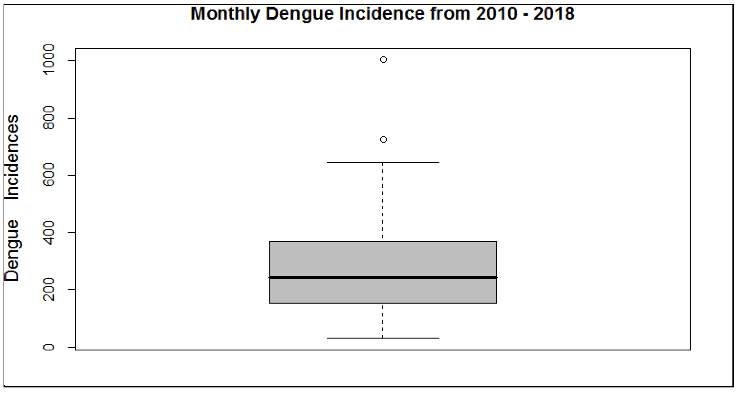
A logistic regression approach was used for model formulation. The response variable was defined as whether the monthly dengue incidences were above the median dengue incidence (1) or not (0) for the entire time period (2010–2018). Figure 1 shows the boxplot of monthly dengue incidences from 2010 to 2018. From Figure 1, monthly dengue incidences were skewed towards the right with a couple of outliers. The median was chosen as the threshold for risk since it was not influenced by outliers. A month was considered at risk for higher dengue levels if the dengue count was above the median. The objective was to build a binary logistic regression model to predict whether the month would be at risk for high dengue incidences. Since this variable assumed a value of either 1 or 0, based on whether or not the dengue count is above the median, a logistic regression model could be used for risk prediction of dengue incidence [18]. The predictor variables were the average temperature, rainfall, and average relative humidity. An overview of the logistic regression model follows.
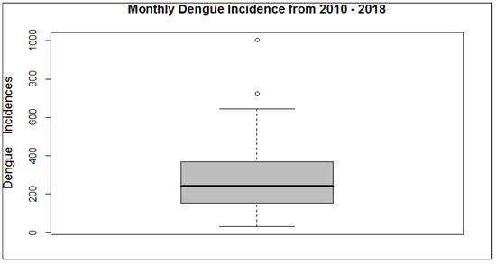
Figure 1.
Boxplot of monthly dengue incidences.
2.2. Overview of the Logistic Regression Model
2.2.1. Logistic Regression
The logistic regression model is a widely used binary data modeling approach that belongs to the family of generalized linear models (GLMs) [18]. In GLMs, each outcome of the response variable is assumed to be generated from a particular distribution in the exponential family including normal, binomial, Poisson, and Gamma distributions. Logistic regression is used to model the relationship between a binary response variable (can assume yes/no, dead/alive, …, etc.) and a set of predictors that can be discrete, continuous, or categorical. Since the response variable is binary, it can take a value of either 0 or 1.
For a binary response variable Y, with Y = 0 or 1, and a single predictor variable x, E(Y|x) = P(Y = 1 |x) is written as a function of x as follows. First, an abbreviation p(x) = P(Y = 1|x) is set, and then p(x) is written as:
This is known as a logistic regression model. Rearranging this equation gives:
The left-hand side of the expression above is called the log odds or logit of p(x). The expression gives the odds that event Y = 1 will occur. For multiple predictor variables, X = x1, x2, x3, …, xk, the logistic regression model becomes:
and the logit becomes:
From the above expression, is the change in log odds of Y = 1 that occurs for one unit increase in xi, while other predictors are fixed. Simple algebra can be used to show that is the odds ratio associated with a one unit increase in predictor xi. An interpretation of this odds ratio is that for each one-unit increment of xi, while holding other predictors as fixed, the percentage change (increase/decrease) of odds for Y occurring is − 1.
The logistic regression method assumes following:
- the outcome is a binary variable;
- there is a linear relationship between the logit of the outcome and each predictor variable;
- there are no influential values (extreme values or outliers) in the continuous predictors; and
- there is no high intercorrelation (multicollinearity) among predictors.
2.2.2. Estimation of Parameters and Goodness-Of-Fit of the Model
Estimation of parameters and data analysis of the logistic regression model is normally performed using statistical software. In this study, the R software environment was used. The glm() function, with family = “binomial” option, was used to estimate regression parameters and perform the data analysis.
The likelihood ratio test was used to assess the significance of the overall model with k predictors. The null hypothesis was The likelihood ratio test statistic was given by:
where is the log likelihood of the full (fitted) model, and is the log likelihood of the model with only one constant term (reduced model). This test statistic had a chi-square distribution with k degrees of freedom. The test for individual predictors can be done using a z-test. Z statistics and p-values were given in the R regression output. Small p-values indicated the corresponding predictors were significant.
Overall performance of the fitted model can be measured by several different goodness-of-fit tests. Goodness-of-fit tests assess how well the model fits the observed data. Several widely used goodness-of-fit tests and measures for logistic regression are:
- Pearson chi-square goodness-of-fit test,
- Deviance goodness-of-fit test,
- Hosmer–Lemeshow goodness-of-fit test,
- Pseudo R2, and
- Receiver operating characteristic (ROC) curve.
The Pearson chi-square goodness-of-fit test tests the null hypothesis that the chosen model fits the data. The test statistic computes the overall difference between the observed probabilities and those estimated from the fitted model. Nonsignificant (larger p-value) tests indicate that the chosen model is a good fit. This means that the difference between the expected values using this chosen model and the actual values is not significant.
The deviance goodness-of-fit test calculates its test statistic as the sum of the difference between the log likelihood of the saturated model (has as many coefficients as observations in the data set) and the chosen model for the data. It follows a chi-square distribution with degrees of freedom equaling the difference in the number of parameters in the two models. The null hypothesis sets the coefficients that are in the saturated model, but not in the chosen model, to zero. A large p- value indicates that none of the excluded variables are significant; therefore, the fitted model is as good as the saturated model.
The Hosmer–Lemeshow goodness-of-fit test is widely used in logistic regression. It groups observations based on their estimated probabilities and compares the observed and expected counts using chi-square statistics. Smaller differences in expected and observed counts give a smaller test statistic value; therefore, a larger p-value indicates a good fit.
The pseudo R2 statistic is slightly analogous to the coefficient of determination in the linear regression model in that it takes values in the range of 0 to 1. It is defined as:
A larger value indicates a better fit of the model. However, it cannot be interpreted that the amount of variation in Y is explained by the predictor variable X.
ROC Curve, or “receiver operating characteristic curve”, is a way of assessing the prediction capacity of a model. It is a plot of sensitivity versus 1 – specificity for the possible cutoff classification probability values p0. Sensitivity represents the true positive rate and specificity represents the true negative rate. The position of the ROC on the graph reflects the accuracy of the diagnostic test. It covers all possible thresholds (cutoff points). The ROC of random guessing lies on the diagonal line. The ROC of a perfect diagnostic technique is a point at the upper left corner of the graph, where the true positive proportion is 1.0 and the false positive proportion is 0. The area under the ROC curve provides an overall measure of fit of the model. The area under the ROC curve above 0.9 indicates an outstanding model fit. If the area is between 0.8 and 0.9, it is considered to be excellent fit. An area between 0.7 and 0.8 indicates an acceptable fit. An area between 0.5 and 0.7 indicates a poor fit, and area of 0.5 indicates no fit.
Residual plots can be used to better understand the models and diagnose any particular problems. There are many types of residuals such as ordinary residuals (raw residuals), Pearson residuals, deviance residuals, and studentized residuals. They all reflect the difference between fitted and observed values. In a basic type of a residual plot, the residuals are plotted in the order that the data was collected or plotted against either predictors or fitted values. If the model is performing well, random behavior in the residual plot should be noted. Technical details of residual plots are given in [18,19,20].
3. Data Analysis and Discussion of Results
3.1. Data Analysis
The variable “IsRisk” was used to define whether a particular month had a high number of dengue incidences. This variable was the response variable in the logistic regression model. The explanatory variables were monthly average temperature, monthly cumulative rainfall, and monthly average relative humidity. The results are given in Table 1.

Table 1.
Parameters of the logistic regression model.
Based on the above p-values of the model parameters, rainfall was the only climate variable that produced a significant relationship with the IsRisk variable. To investigate this, a boxplot showing the rainfall variable relative to the binary response variable IsRisk was created. The boxplot is depicted in Figure 2. This boxplot also revealed that there was a weak correlation, where larger values of rainfall tended to decrease the likelihood of having above-median dengue incidences. The Pearson correlation coefficient between monthly dengue incidences and rainfall was −0.35804, which also suggested a weak, negative association.
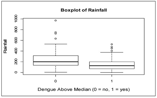
Figure 2.
Boxplot of rainfall relative to risk.
Since it takes a certain period of time for an egg to develop into an adult mosquito, the influence of climate was expected to be visible one or two months later [21]. For this reason, the IsRisk variable was modeled using climate data with one and two lag-months. For one lag-month data, the Pearson correlation coefficient between dengue incidences and rainfall was 0.08190758 (p > 0.05), indicating no significant association. For two lag-months data, the correlation coefficient was 0.3987109 (p < 0.05), indicating a significant positive association.
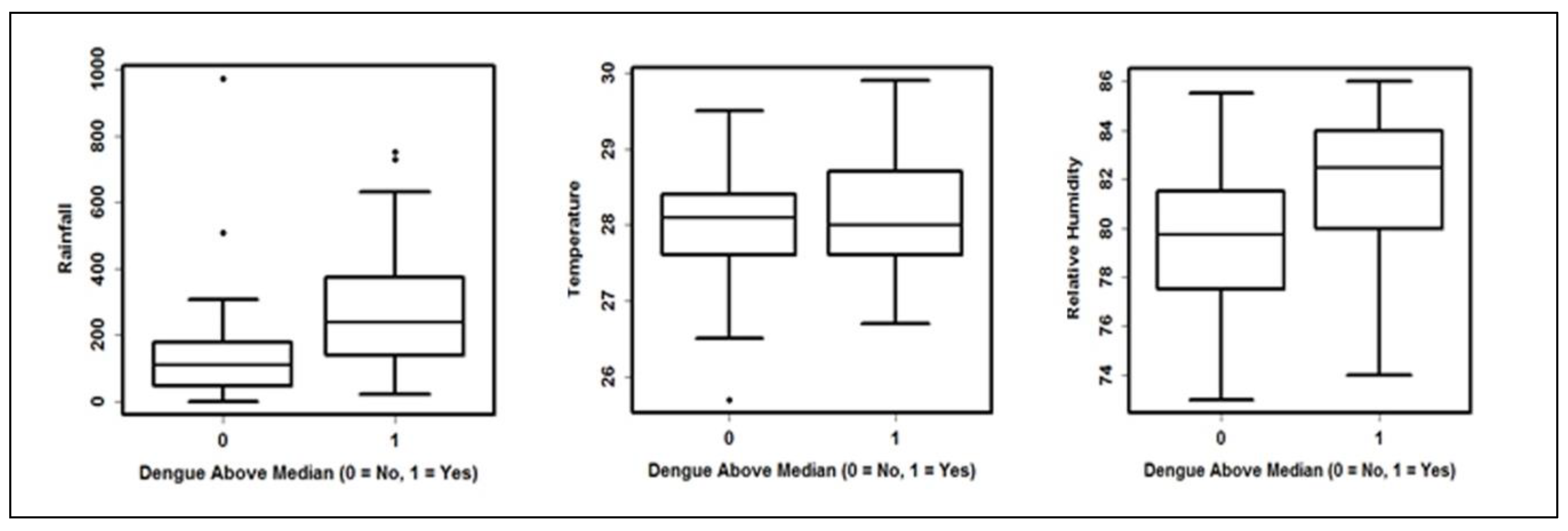
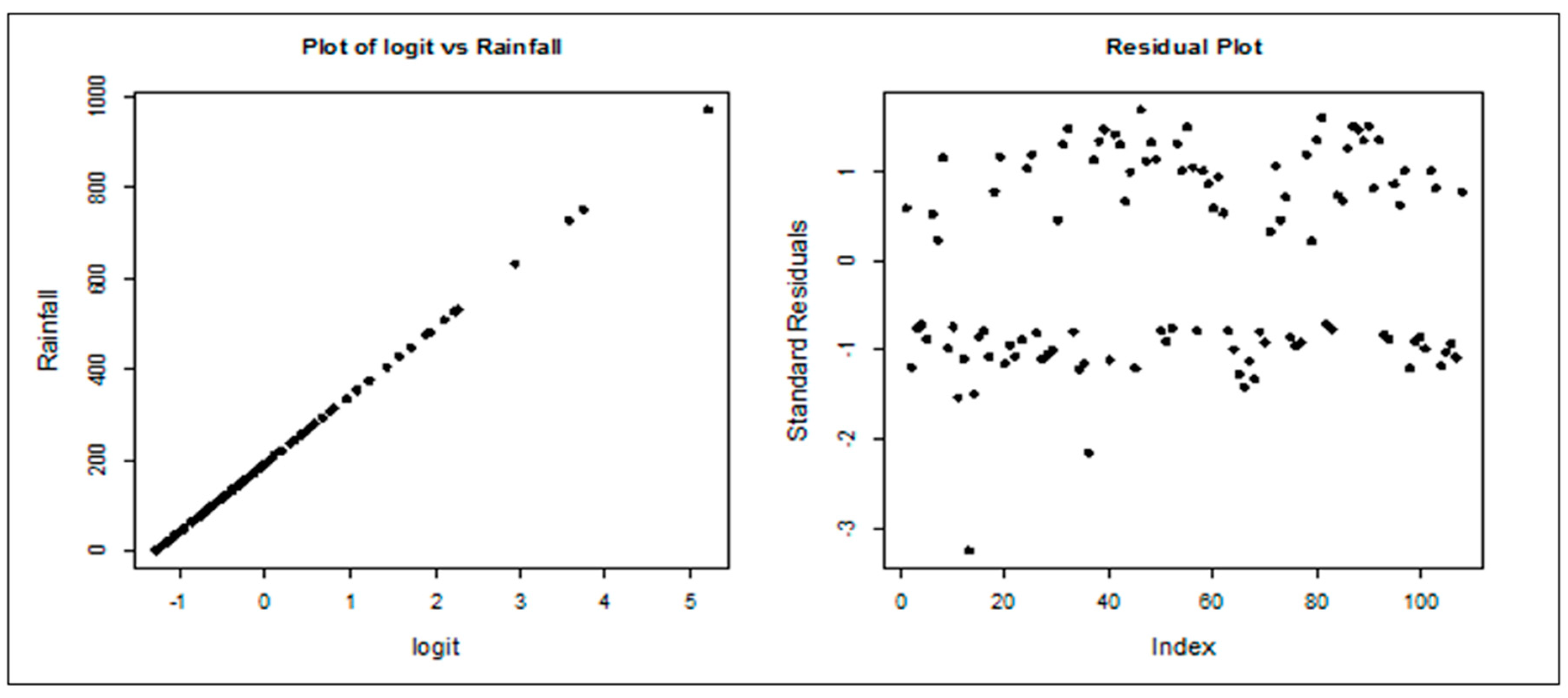
From here onwards, the two lag-months data were considered for analysis. First, boxplots of three climate variables relative to the binary variable IsRisk were created. Figure 3 shows these boxplots. Based on these boxplots, rainfall had an effect on the likelihood of having high dengue incidences. Larger values of rainfall tended to increase the likelihood of having above-median dengue incidences. From the other two boxplots in Figure 3, temperature and relative humidity did not affect the likelihood of having high dengue incidences. These findings were confirmed in the logistic regression output. A logistic regression model for the IsRisk variable was fitted based on these three climate variables. The only significant variable affecting the likelihood of having high dengue incidences was rainfall. Therefore, non-significant climate variables, average temperature, and average relative humidity were dropped from the model. Then the model was fitted so that the relationship was between the IsRisk variable and rainfall. First, the assumptions of logistic regression were checked for this model. The first assumption, that the outcome was a binary variable, was already satisfied. Then, the last assumption, that there was no high multicollinearity among predictors, was not applicable since there was only one predictor now. The second assumption required a linear relationship between the logit and predictors. Figure 4 shows this relationship and depicts it to be linear. The third assumption required no influential values in the predictors. From the residual plot in Figure 4, all residuals except one were between −3 and 3. Only one residual was very close to −3. From these residuals it can be concluded that no influential values were present in the rainfall data. In conclusion, it was verified that all assumptions for the logistic regression model were satisfied.
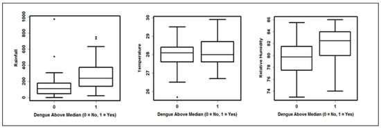
Figure 3.
Boxplots of climate variables relative to risk (two month lag data).
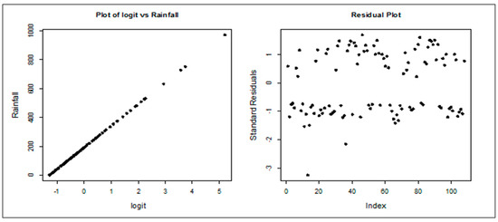
Figure 4.
Plot of logit vs. rainfall and the residual plot.
Table 2 gives the parameter estimates of the logistic regression model. The p-value (<0.05) showed a significant, positive association between rainfall and the likelihood of having high dengue incidences. The likelihood ratio test, with a p-value of 0, indicated the suitability of the model.
Table 2.
Parameters of the logistic regression model.
Now, the widely used Hosmer–Lemeshow goodness-of fit-test was used to assess model adequacy. The p-value of the test was 0.07965 (>0.05). Based on this p-value at a 0.05 significance level, it can be concluded that the model was adequate for use.
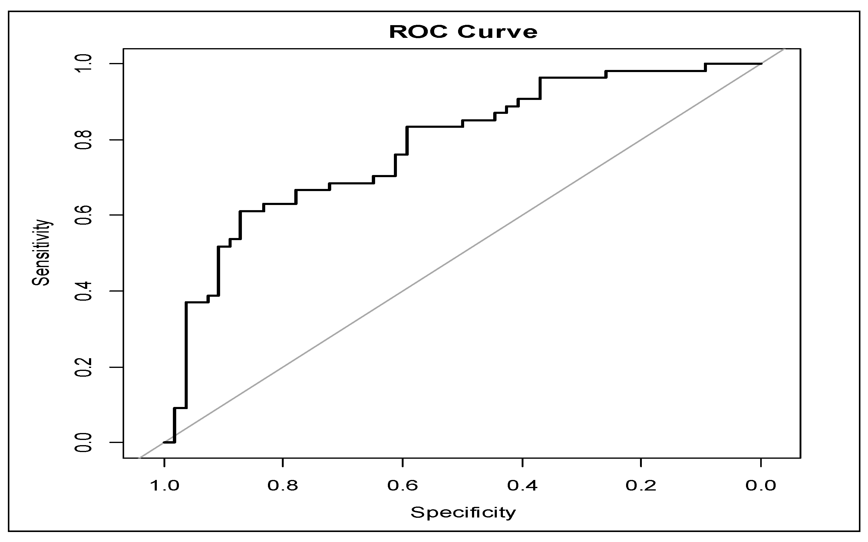
Figure 5 shows a sketch of the ROC curve for the logistic regression model. The area under the curve was 0.7816, with 95% confidence interval ranging from 0.6946 to 0.8685. This was in the range of acceptable to excellent model fit.
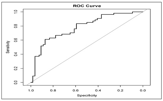
Figure 5.
Receiver operating characteristic (ROC) curve.
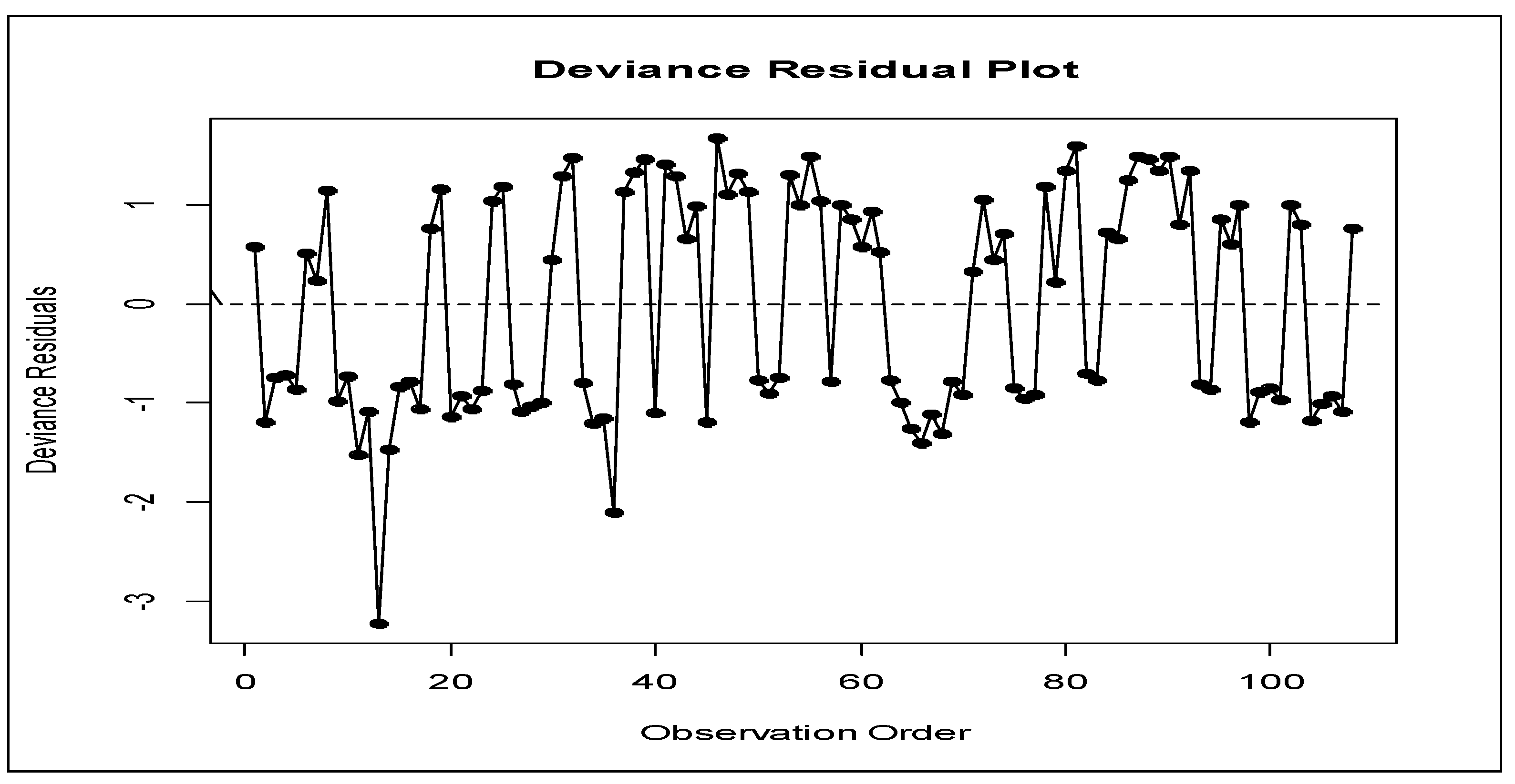
As indicated earlier, residual plots can be used to diagnose any problems in the model. The standard residual plot was already checked in checking the assumptions of the model. It was noted that the residual plot did not indicate any serious violations of assumptions. Here, the deviance residuals versus order plot were also created, given in Figure 6. Residuals fell randomly around the centerline without any apparent trends or patterns. This deviance residual plot did not suggest any major problems with the model.
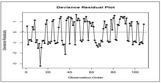
Figure 6.
Deviance residual plot.
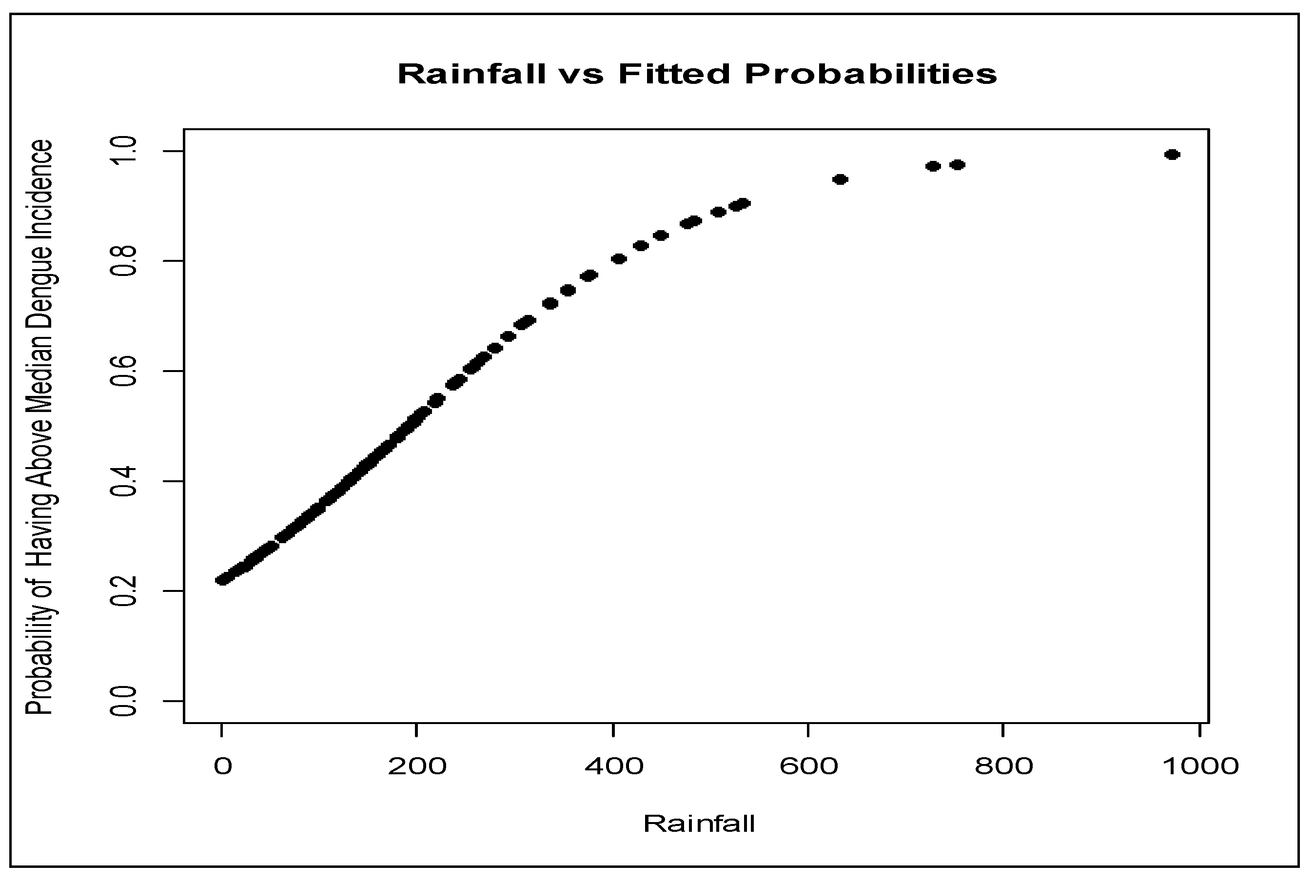
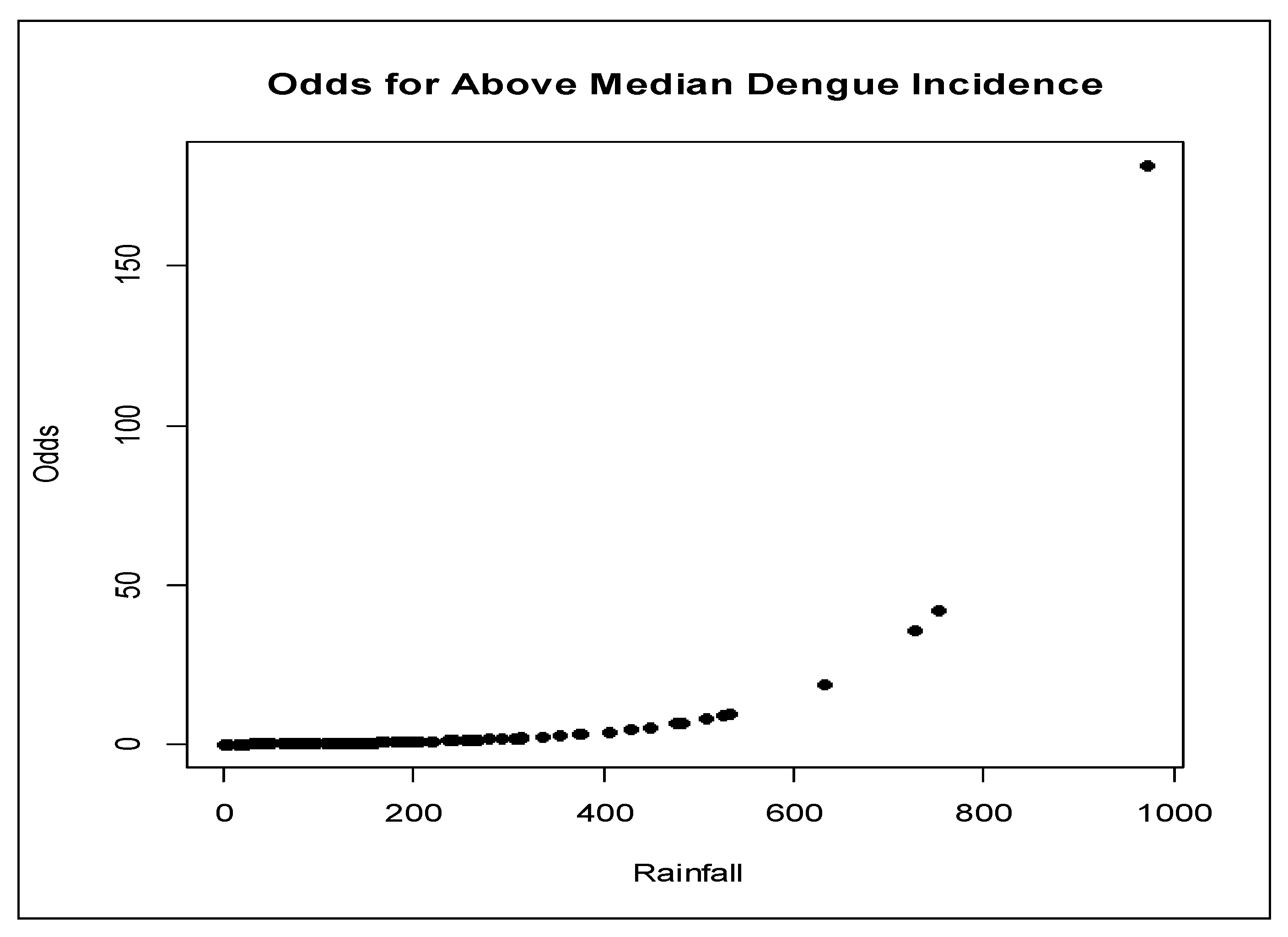
In Figure 7, the fitted probabilities of having above-median dengue incidences were plotted against the rainfall. The positive association between the rainfall and the likelihood of having above-median dengue incidences was evident in the plot. As rainfall increased, the likelihood increased. Figure 8 shows the relationship between odds for having high dengue incidences and the rainfall. This plot shows that when rainfall was low, the odds of having dengue incidences above the median were lower, and as rainfall increased, the odds were significantly higher. For example, if the amount of rainfall was 400 mm, the odds were about four times higher for having above-median dengue incidences for that month.

Figure 7.
Fitted probabilities against rainfall.

Figure 8.
Odds against rainfall.
3.2. Interpreting Coefficients
Rainfall was the only significant predictor that affected the likelihood of having higher dengue incidences. Furthermore, the logistic regression model with two lag-months of rainfall data was the best model to fit the data. This prediction model was then used to interpret model coefficients. In Table 2, regression coefficients and p-values for this particular model were shown. Rainfall was significant (p-value was nearly zero) with the regression coefficient = 0.00666. This meant for every one unit (mm) increase in the amount of monthly rainfall, the odds for having dengue incidences above the median after a period of two months increased by (exp(0.00666) − 1)% = 0.69%. In other words, for each one mm rise in rainfall, the odds for high dengue incidences in two months were expected to increase by 0.69%. For every 10 mm rise in rainfall, the odds were expected to increase by 6.89%.
The logistic regression model for log odds of having above-median dengue incidences is given by:
where x is the rainfall amount, and p(x) is the probability of having above median dengue incidences. Simplifying this expression gives the model for the probability of having above-median dengue incidences as:
This model calculates the probability of having dengue incidences above the median for a month based on a two lag-month rainfall amount. This model can be considered a risk prediction model for a month based on rainfall. For example, if the rainfall amount was 300 mm for a month, then the probability of having above-median dengue incidences in two months would be 0.6751. This meant there was a 67.51% chance that the month would be at risk of having high dengue incidences.
3.3. Discussion
Being a tropical country, Sri Lanka’s weather is dominated by rainy seasons on a yearly basis. This study found that rainfall significantly affected the likelihood of having high dengue incidences. Furthermore, two lag-months of rainfall influenced the chances of dengue incidence. Since it takes several weeks for an egg to develop into adult mosquito, the influence of climate is expected to be visible one or two months later. Once adult mosquitos have emerged, climate factors affect their survival. The increase in mosquito population is due to the rainfall, and the subsequent increase in dengue incidences has been reported in previous studies [22]. However, a risk prediction model for dengue transmission has not been reported.
Initially, a logistic regression model was considered to investigate the relationship between the likelihood of having higher dengue incidences and three climate variables: average temperature, rainfall, and average relative humidity. That model revealed that the only significant variable was the rainfall. Then, the two nonsignificant variables were dropped from the model. The Pearson correlation coefficient and the scatterplot between the current month’s rainfall and dengue incidences showed a weak, negative relationship. The Pearson correlation coefficient and the scatterplot between dengue incidences and two lag-months rainfall data showed a significant, positive relationship. Then, the logistic regression model was fitted to the relationship between the likelihood of whether or not there was a high dengue incidence over a two-month lag in rainfall. The likelihood ratio test and other goodness of fit tests and measures confirmed that the model was adequate for prediction. Based on the logistic regression model, a risk prediction model was developed for higher dengue incidences based on two lag-months of rainfall data.
This study showed a significant, positive effect between the likelihood of having higher dengue incidences and rainfall. Several previous studies conducted in other parts of the world indicated a positive association between dengue incidences and climate factors [23]. The positive effect from rainfall is justifiable because rain water from water pools provide breeding grounds for mosquitos. That increases the mosquito density, which in turn leads to an increase in dengue incidence rates and the risk of spreading infection among the public. The dengue incidences and the risk may also be associated with socioeconomic levels and dengue control measures implemented by the relevant authorities. These factors were not considered in this study.
4. Conclusions
Dengue has been a critical public health problem in Colombo as well as other parts of Sri Lanka. The objective of this study was to build a model for predicting the likelihood of having high dengue incidences based on climate factors. This study focused on the city of Colombo. The study used monthly data from 2010 to 2018. A logistic regression model was used to fit the data. The results suggested that rainfall was the only significant factor that affected the likelihood of having higher dengue incidences. Having “above-median dengue incidences” was interpreted as the risk of higher dengue incidences. Furthermore, the influence of rainfall on dengue incidences is expected to be visible after some lag-months. This model can be used to predict the likelihood of having high dengue incidences based on rainfall. These finding are helpful for authorities so they can take necessary action in safeguarding the community from dengue outbreaks.
Funding
This research received no external funding.
Conflicts of Interest
The authors declare no conflict of interest.
References
- CDC. Centers for Disease Control and Prevention. Available online: https://www.cdc.gov/dengue/index.html (accessed on 15 March 2019).
- Endy, T.P.; Anderson, K.B.; Nisalak, A.; Yoon, I.K.; Green, S.; Rothman, A.L.; Thomas, S.J.; Jarman, R.G.; Libraty, D.H.; Gibbons, R.V. Determinants of inapparent and symptomatic dengue infection in a prospective study of primary school children in Kamphaeng Phet, Thailand. PLoS Negl. Trop. Dis. 2011, 5. [Google Scholar] [CrossRef] [PubMed]
- World Mosquito Program. Available online: http://www.eliminatedengue.com/our-research/dengue-fever (accessed on 10 March 2019).
- Gubler, D.J. Dengue and dengue hemorrhagic fever. Clin. Microbial. Rev. 1998, 11, 480–496. [Google Scholar] [CrossRef]
- Sirisena, P.P.N.N.; Noordeen, F. Evolution of Dengue in Sri Lanka—Changes in the Virus, Vector, and Climate. Int. J. Infect. Dis. 2014, 19, 6–12. [Google Scholar] [CrossRef] [PubMed]
- International Federation of Red Cross And Red Crescent Societies: Sri Lanka/Dengue DREF Final Report (MDRLK007). Available online: https://reliefweb.int/report/sri-lanka/sri-lanka-dengue-dref-final-report-mdrlk007 (accessed on 20 March 2019).
- Epidemiology Unit of Ministry of Health of Sri Lanka. Available online: http://www.epid.gov.lk/web/ (accessed on 10 March 2019).
- Wu, P.C.; Guo, H.R.; Lung, S.C.; Lin, C.Y.; Su, H.J. Weather as an effective predictor for occurrence of dengue fever in Taiwan. Acta Tropica. 2007, 103, 50–57. [Google Scholar] [CrossRef] [PubMed]
- Chandrakantha, L. Statistical analysis of climate factors influencing dengue incidences in Colombo, Sri Lanka: Poisson and negative binomial regression approach. Int. J. Sci. Res. Publ. 2019, 9, 133–144. [Google Scholar] [CrossRef]
- Goto, K.; Kumarrendran, B.; Mettananda, S.; Gunasekara, D.; Fujii, Y.; Kaneko, S. Analysis of Effects of Meteorological Factors on Dengue Incidence in Sri Lanka Using Time Series Data. PLoS ONE 2013, 8. [Google Scholar] [CrossRef] [PubMed]
- Withanage, G.P.; Wishwakula, S.D.; Gunawardena, Y.I.; Hapugoda, M.D. A Forecasting Model for Dengue Incidence in the District of Gampaha, Sri Lanka. Parasit. Vector. 2018, 11. [Google Scholar] [CrossRef] [PubMed]
- Kavinga, H.W.B.; Jayasundara, D.D.M.; Jayakody, D.K.N. A New Dengue Outbreak Statistical Model using the Time Series Analysis. Eur. Int. J. Sci. Technol. 2013, 2, 35–52. [Google Scholar]
- Sun, W.; Xue, L.; Xie, X. Spatial-temporal Distribution of Dengue and Climate Characteristics for Two Clusters in Sri Lanka from 2012 to 2016. Sci. Rep. 2017, 7, 12884. [Google Scholar] [CrossRef] [PubMed]
- Iguchi, A.; Seposo, X.T.; Honda, Y. Meteorological Factors Affecting Dengue Incidence in Davao, Philippines. BMC Pub. Health 2018, 18, 629. [Google Scholar] [CrossRef] [PubMed]
- Campbell, K.M.; Lin, C.; Iamsirithawom, S.; Scott, T.W. The complex relationship between weather and dengue virus transmission in Thailand. Am. J. Trop. Med. Hyg. 2013, 89, 1066–1080. [Google Scholar] [CrossRef] [PubMed]
- Vu, H.H.; Okumura, J.; Hashizume, M.; Tran, D.N.; Yamamoto, T. Regional differences in the growing incidences of dengue fever in Vietnam explained by weather variability. Trop. Med. Health 2014, 42, 25–33. [Google Scholar] [CrossRef] [PubMed]
- Department of Census and Statistics of Sri Lanka. Available online: http://www.statistics.gov (accessed on 10 March 2019).
- Hosmer, D.W., Jr.; Lemeshow, S. Applied Logistic Regression, 3rd ed.; John Wiley & Sons, Inc.: New York, NY, USA, 2013. [Google Scholar]
- Cordeiro, G.M.; Simas, A.B. The distribution of Pearson residuals in generalized linear models. Comput. Stat. Data Anal. 2009, 53, 3397–3411. [Google Scholar] [CrossRef]
- Menard, S. Applied Logistic Regression Analysis, 2nd ed.; SAGE Publications: New York, NY, USA, 2001. [Google Scholar]
- Nakhapakorn, K.; Tripathi, N.K. An Information Value Based Analysis of Physical and Climatic Factors Affecting Dengue Fever and Dengue Haemorrhagic Fever Incidence. Int. J. Health Geogr. 2005, 4. [Google Scholar] [CrossRef] [PubMed]
- Focks, D.; Barrera, R. Report on Scientific Working Group Meeting on Dengue. Geneva: WHO: 2007 Dengue Transmission Dynamics: Assessment and Implications for Control. 2007, pp. 92–108. Available online: https://www.who.int/tdr/publications/documents/swg_dengue_2.pdf (accessed on 7 March 2019).
- Choi, Y.; Tang, C.S.; McIve, L.; Hashizume, M.; Chan, V.; Abeyasinghe, R.R.; Iddings, S.; Huy, R. Effects of Weather Factors on Dengue Fever Incidence and Implications for Interventions in Cambodia. BMC Public Health 2016, 16. [Google Scholar] [CrossRef] [PubMed]

© 2019 by the author. Licensee MDPI, Basel, Switzerland. This article is an open access article distributed under the terms and conditions of the Creative Commons Attribution (CC BY) license (http://creativecommons.org/licenses/by/4.0/).