Setting Alarm Thresholds in Measurements with Systematic and Random Errors

Abstract

For statistical evaluations that involve within-group and between-group variance components (denoted ${\sigma }_W^2$ and ${\sigma }_B^2$, respectively), there is sometimes a need to monitor for a shift in the mean of time-ordered data. Uncertainty in the estimates ${\widehat{\sigma }}_W^2$ and ${\widehat{\sigma }}_B^2$ should be accounted for when setting alarm thresholds to check for a mean shift as both ${\sigma }_W^2$ and ${\sigma }_B^2$ must be estimated. One-way random effects analysis of variance (ANOVA) is the main tool for analysing such grouped data. Nearly all of the ANOVA applications assume that both the within-group and between-group components are normally distributed. However, depending on the application, the within-group and/or between-group probability distributions might not be well approximated by a normal distribution. This review paper uses the same example throughout to illustrate the possible approaches to setting alarm limits in grouped data, depending on what is assumed about the within-group and between-group probability distributions. The example involves measurement data, for which systematic errors are assumed to remain constant within a group, and to change between groups. The false alarm probability depends on the assumed measurement error model and its within-group and between-group error variances, which are estimated while using historical data, usually with ample within-group data, but with a small number of groups (three to 10 typically). This paper illustrates the parametric, semi-parametric, and non-parametric options to setting alarm thresholds in such grouped data.

1. Introduction

Many applications involve testing for a shift in the mean of a probability distribution for a random quantity. Any such test will have a false alarm probability (FAP) and a failure-to-detect-the-shift probability. This review paper uses the same example application throughout to illustrate the possible approaches to setting alarm thresholds in measurement data that have both systematic and random error components. The International Atomic Energy Agency (IAEA) verification data that are collected to monitor for possible nuclear material diversion is the example [1,2]. Such verification data from IAEA inspections often consist of paired data (usually operators’ declarations and inspectors’ verification results) that are analyzed to detect the significant differences. Any significant difference could arise due to a problem with the operator and/or inspector measurement systems, or due to the operator falsifying the data in an attempt to mask diversion; such a falsification would cause a mean shift between the operator declaration and the corresponding inspector measurement. Paired data from past inspections are used to estimate the alarm limits, and each inspection period is regarded as a group within which the measurements are assumed to have the same systematic error due to calibration and other effects [1,2,3]. The corresponding FAP depends on the assumed measurement error model and its random (within-group) and systematic (between-group) error variances, which are estimated while using data from previous inspections [3].

This paper reviews the parametric, semi-parametric, and non-parametric options for setting alarm thresholds in such grouped data. If both the within-group and between-group measurement errors have approximately normal distributions, then a parametric option that involves tolerance intervals [4,5,6,7,8,9,10,11] for one-way ANOVA can be used. If either or both error distributions are not close to normal, then a semi-parametric method that is based on a Dirichlet process mixture [12] can be applied. A non-parametric method [13] could be used if there is enough data.

2. Materials and Methods

An effective measurement error model for operator and inspector data must account for variation within and between groups, where a group is, for example, a calibration period, inspection period, item, or laboratory. In this paper, a group is an inspection period. A typical model that assumes additive errors for the inspector (I) (and similarly for the operator O) is

$$I_{jk}={\mu }_{jk}+S_{Ij}+R_{Ijk}$$

(1)

where for item k (from 1 to n) in group j (from 1 to g), $I_{jk}$ is the inspector’s measured value of the true but unknown value ${\mu }_{jk}$, $R_{Ijk}~N(0,{\sigma }_{RI}^2)$ is a random error, and $S_{Ij}~N(0,{\sigma }_{SI}^2)$ is a short-term systematic error that arises due to metrology changes, most important of which is recalibration between inspection periods [1,2,3,14]. For a fixed value of ${\mu }_{jk},$ the total variance of the inspector measurement is ${\sigma }_I^2$ = ${\sigma }_{SI}^2+{\sigma }_{RI}^2$.

The measurement error model in Equation (1) sets the stage for applying ANOVA with random effects [2,15,16,17,18,19,20]. Neither $R_{Ijk}$ nor $S_{Ij}$ are observable. If the errors tend to scale with the true value, then a typical model for multiplicative errors (with relative standard deviations (RSD) ${\delta }_S$ and ${\delta }_R)$ is

$$I_{jk}={\mu }_{jk}(1+{\tilde{S}}_{Ij}+{\tilde{R}}_{Ijk})$$

(2)

where ${\tilde{S}}_{Ij}~N(0,{\delta }_{SI}^2)$, ${\tilde{R}}_{Ijk}~N(0,{\delta }_{RI}^2)$. As explained below, for a technical reason, the data model in Equation (2) is slightly modified from normal distributions to truncated normal distributions in the IAEA application. Let ${\delta }_R^2={\delta }_{RO}^2+{\delta }_{RI}^2$ and ${\delta }_S^2={\delta }_{SO}^2+{\delta }_{SI}^2$. For a fixed value of ${\mu }_{jk},$ the total variance of the inspector measurement is ${\sigma }_I^2$ = ${\sigma }_{SI}^2+{\sigma }_{RI}^2={\mu }_{jk}^2\left({\delta }_{SI}^2+{\delta }_{RI}^2\right)$. Let $O_{jk}={\mu }_{jk}\left(1+{\tilde{S}}_{Oj}+{\tilde{R}}_{Oj}\right)$ and $I_{jk}={\mu }_{jk}\left(1+{\tilde{S}}_{Ij}+{\tilde{R}}_{Ij}\right)$. Subsequently, the assumed model for the relative difference between operator and inspector is

$$\frac{{\mu }_{jk}(1+{\tilde{S}}_{Oj}+{\tilde{R}}_{Ojk})-{\mu }_{jk}(1+{\tilde{S}}_{Ij}+{\tilde{R}}_{Ijk})}{{\mu }_{jk}}={\tilde{S}}_j+{\tilde{R}}_{jk}$$

(3)

for the operators declared value of item $k$ from group $j,$ ${\tilde{R}}_{jk}={\tilde{R}}_{Ojk}-{\tilde{R}}_{Ijk}~N\left(0,{\delta }_R^2\right)$ is the net random error and ${\tilde{S}}_j={\tilde{S}}_{Oj}-{\tilde{S}}_{Ij}~N\left(0,{\delta }_S^2\right)$ is the net short-term systematic error. In practice, while assuming no data falsification by the operator, Equation (3) can be calculated using the relative differences, $d_{jk}=\frac{o_{jk}-i_{jk}}{o_{jk}},$ where $o_{jk}$ is used in the denominator to estimate ${\mu }_{jk}$, because typically ${\delta }_{SO}^2+{\delta }_{RO}^2\le {\delta }_{SI}^2+{\delta }_{RI}^2$, with ${\delta }_{TO}=\sqrt{{\delta }_{SO}^2+{\delta }_{RO}^2}$ always being very small, 0.02 or less, in the IAEA application. Formally, a ratio of normal random variables has infinite variance [3,21]. To define a ratio that has finite variance, a truncated normal can be used as the data model in Equation (2) for $o_{jk}$ in $d_{jk}=1-\frac{i_{jk}}{o_{jk}},$ which is equal in distribution to $1-\frac{{\mu }_{jk}(1+{\delta }_{TI}{z}_1)}{{\mu }_{jk}(1+{\delta }_{TO}{z}_2)}=1-R$, which involves a ratio $R=\frac{(1+{\delta }_{TI}{z}_1)}{(1+{\delta }_{TO}{z}_2)}$ of the independent normal random variables $z_1$ and $z_2$ (for the case of one measurement per group; multiple measurements per group is treated similarly). Note that the unknown true value ${\mu }_{jk}$ cancels in $R$, and then specifically, replace ${\delta }_{TO}{z}_2$ with, for example, the conditional normal random variable ${\delta }_{TO}{\tilde{z}}_2={\delta }_{TO}{z}_2\left|\right\{{\delta }_{TO}{z}_2>-0.5\}$. The value −0.5 is an arbitrary but reasonable truncation value that is at least 25 standard deviations from the mean, and so such truncation would only take effect for a random realized value that is 25 or more standard deviations ${\delta }_{TO}$ from the mean (an event that occurs with almost zero probability). The modified ratio then has finite moments of all orders, because the numerator has a normal distribution and the denominator is an independent truncated normal that is no smaller than 0.5 (so the mean of the ratio cannot exceed twice the mean of the numerator, and similarly for other moments). Therefore, because ${\delta }_{TO}\le 0.02$ and ${\delta }_{TI}\le 0.05$ (typically), the distribution of the values $d_{jk}=\frac{o_{jk}-i_{jk}}{o_{jk}}$ is guaranteed to have finite moments when the data model for $o_{jk}$ is a truncated normal, such as just described. In addition, provided ${\delta }_{TO}\le 0.02$ and ${\delta }_{TI}\le 0.05,$ the distribution of the truncated version of the ratio $d_{jk}=\frac{o_{jk}-i_{jk}}{o_{jk}}$ is extremely close to a normal distribution (see Supplementary 1, and also see Section 5 and Section 6 for cases in which the distribution of $d_{jk}=\frac{o_{jk}-i_{jk}}{o_{jk}}$ does not appear to be approximately normal). Additionally, the expression for the approximate variance ${\delta }_d^2={\delta }_{SO}^2+{\delta }_{RO}^2+{\delta }_{SI}^2+{\delta }_{RI}^2$ of $d_{\mathrm{rel}}=(O-I)/O$ arising from using linear error variance propagation is accurate for quite large ${\delta }_T$, up to approximately ${\delta }_T=\sqrt{{\delta }_{TO}^2+{\delta }_{TI}^2}$ = 0.20, where. ${\delta }_{TO}=\sqrt{{\delta }_{RO}^2+{\delta }_{SO}^2}$ (as confirmed by simulations in R [20], and see [3,21]). In addition, the simulation-based tolerance intervals in Section 4, Section 5 and Section 6 are constructed by simulating the ratio of a normal to a truncated normal, so all of the simulation results are accurate for $R=\frac{(1+{\delta }_{TI}{z}_1)}{(1+{\delta }_{TO}{\tilde{z}}_2)}$ (with a truncated data model for the denominator, as described above) to within very small simulation error arising from performing a finite but large number of simulations. To summarize this issue regarding a ratio of normal random variables, the parametric option using simulation assumes, as discussed, that the truncated ratio $R=\frac{(1+{\delta }_{TI}{z}_1)}{(1+{\delta }_{TO}{\tilde{z}}_2)}$, involves a normal distribution for the numerator and a truncated normal for the denominator; and, in many real data sets, this assumption is reasonable on the basis of normality checks. However, because $R=\frac{(1+{\delta }_{TI}{z}_1)}{(1+{\delta }_{TO}{\tilde{z}}_2)}$ might not always appear to be approximately normally distributed, this paper also considers the semi-parametric and non-parametric alternatives to calculating alarm thresholds for the truncated version of $d_{jk}$ in Section 5 and Section 6, respectively.

In some applications, all four error variance components must be estimated [1,2,3,17,18,19], but in this application, only the aggregate variances ${\delta }_S^2$ and ${\delta }_R^2$ need to be estimated. This paper’s focus is on the total relative variance, ${\delta }_T^2={\delta }_S^2+{\delta }_R^2$, because $d_{ij}~N\left(0,{\delta }_T^2\right)$ (approximately, due to using $d_{jk}=\frac{o_{jk}-i_{jk}}{o_{jk}}$ rather than $d_{jk}=\frac{o_{jk}-i_{jk}}{{\mu }_{jk}}$). The estimated variances ${\widehat{\delta }}_R^2$ and ${\widehat{\delta }}_S^2$ are used to compute ${\widehat{\delta }}_T^2={\widehat{\delta }}_S^2+{\widehat{\delta }}_R^2$, so that ${\widehat{\delta }}_T$ can be used to set an alarm threshold for future $d_{\mathrm{rel}}$ value. Specifically, in future values of the operator-inspector difference statistic $d_i=(o_i-i_i)/o_i$, if $\left|d_i\right|>k{\widehat{\delta }}_T$ (in two-sided testing), then the i-th item selected for verification leads to an alarm, where ${\widehat{\delta }}_T=\sqrt{{\widehat{\delta }}_R^2+{\widehat{\delta }}_S^2,}$ (with ${\delta }_T$ the total RSD, ${\delta }_S$ the between-period short-term systematic error RSD, and ${\delta }_R$ the within-period reproducibility) and k = 3 is a common current choice that corresponds to a small $\alpha$ of approximately 0.003 if ${\widehat{\delta }}_T$ = ${\delta }_T$.Therefore, the focus of this paper is a one-way random effects ANOVA [16]. Regarding jargon, note that the short-term systematic errors are fixed within an inspection period, but they are random across periods, so this is called a random effects ANOVA model [15]. Due to the estimation error in ${\widehat{\delta }}_T$, the actual FAP can be considerably larger than 0.05, as shown in Section 4.

The usual ANOVA decomposition is

$${\displaystyle \sum _{j=1}^g{\displaystyle \sum _{k=1}^n(d_{jk}-{\overline{d}}_{··}}{)}^2=}{\displaystyle \sum _{j=1}^g{\displaystyle \sum _{k=1}^n(d_{jk}-{\overline{d}}_{k·}}{)}^2+}n{\displaystyle \sum _{j=1}^g{({\overline{d}}_{j·}-{\overline{d}}_{··})}^2}=SSW+SSB=S_W^2+S_B^2$$

(4)

where $d_{jk}=o_{jk}-i_{jk}$ for additive models and $d_{jk}=(o_{jk}-i_{jk})/o_{jk}$ for multiplicative models as assumed from now on (to avoid cluttering the notation, the “rel” subscript in $d_{\mathrm{rel}}=(O-I)/O$ is omitted). In Equation (4), SSW is the within group sum of squares, and SSB is the between group sum of squares. For simplicity, Equation (4) assumes that each group has the same number of measurements n. As usual in one-way (one grouping variable) random effects ANOVA, $E({\displaystyle \sum _{j=1}^g{\displaystyle \sum _{k=1}^n(d_{jk}-{\overline{d}}_{j·}}{)}^2)/(ng-1)=}{\delta }_R^2$ and $E(\frac{n}{g-1}{\displaystyle \sum _{j=1}^g{({\overline{d}}_{j·}-{\overline{d}}_{··})}^2})=n{\delta }_S^2+{\delta }_R^2$, so ${\widehat{\delta }}_R^2=\frac{S_W^2}{g(n-1)}$ and ${\widehat{\delta }}_S^2=\frac{S_B^2/(g-1)-S_W^2/(g(n-1))}{n}$.

For data sets in which $d_{jk}$ appears to have approximately a normal distribution, key properties (such as the variances, see Supplementary 1) of the estimators ${\widehat{\delta }}_R^2$ and ${\widehat{\delta }}_S^2$ are approximately known [15,16]. However, biased estimators can have smaller mean squared error (MSE), so other estimators should be considered. Additionally, again assuming normally distributed R and S values, an exact confidence interval (CI) can be constructed for ${\delta }_R^2$ using the ${\chi }_{df=g(n-1)}^2$ distribution, but there are only approximate methods to construct CIs for ${\delta }_S^2$, because the distribution of ${\widehat{\delta }}_S^2$ is a difference of two independent ${\chi }^2$ random variables. Kraemer [11] proposes a modified CI construction method for ${\delta }_S^2$ and investigates impacts of non-normality.

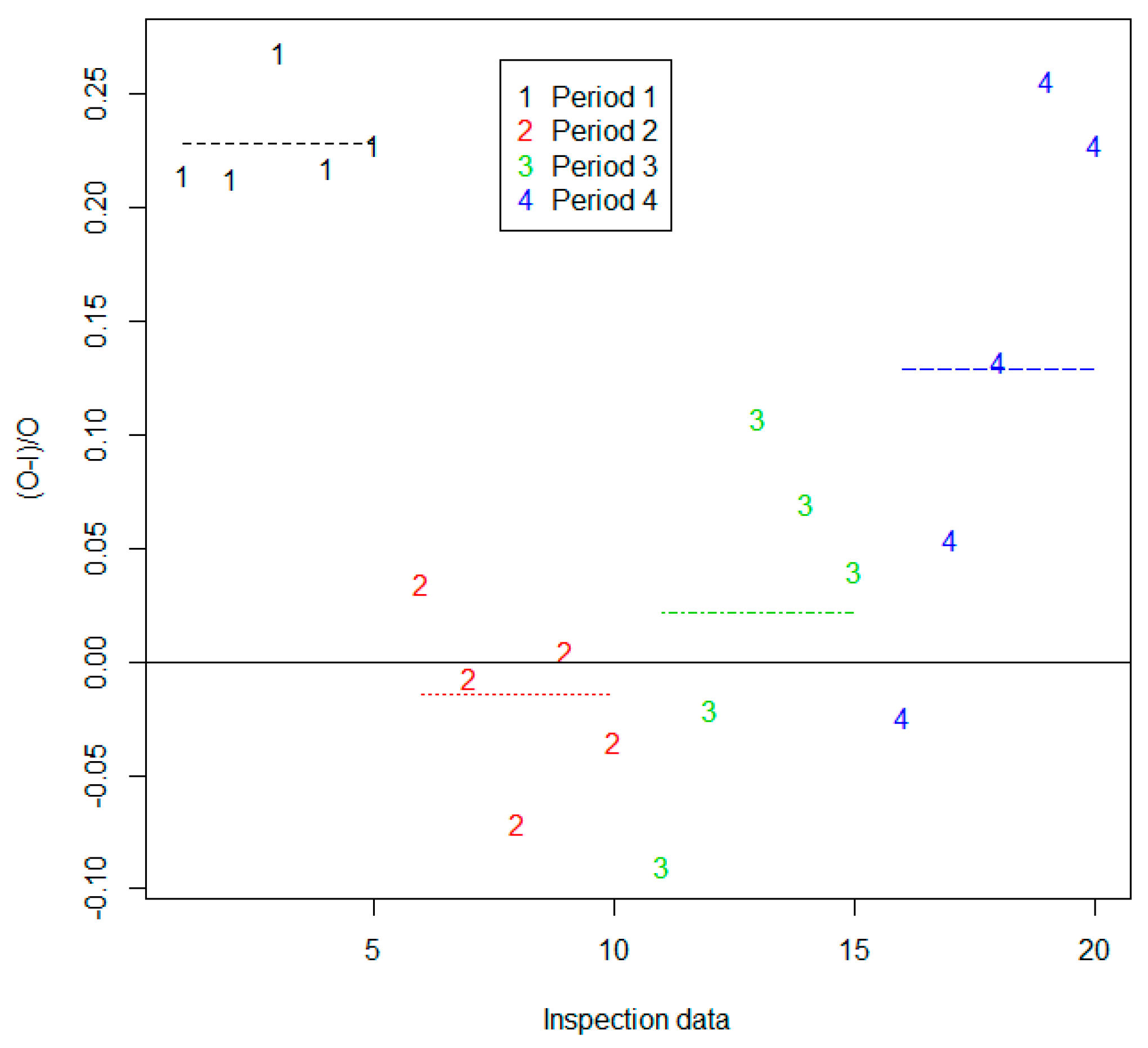
Figure 1 plots 10 realistic simulated $d=\frac{o-i}{o}$ values in each of the three groups of paired (O, I) data. All of the simulations and analyses are done in R [20]. The alarm limit on the right side of the plot in Figure 1 is estimated on the basis of the g = 3 sets of n = 10 values of d. Burr et al. [3] evaluates impacts on alarm probabilities of using estimates of ${\delta }_R^2$ and ${\delta }_S^2$ instead of the true quantities. As in Figure 1, in some data sets, the between-group variation is noticeable when compared to the within-group variation. Figure 2 is the same type of plot as Figure 1, but it is for real data consisting of n = 5 paired comparisons in each of the four inspection periods (groups). For the 30 simulated $d=\frac{o-i}{o}$ values in Figure 1, the estimated RSDs are ${\widehat{\delta }}_R=0.009,{\widehat{\delta }}_S=0.007,{\widehat{\delta }}_T=0.012$ and the true values used in the simulation are ${\delta }_R=0.01,{\delta }_S=0.01,{\delta }_T=0.014.$ For the 20 $d=\frac{o-i}{o}$ values in Figure 2, the estimated RSDs are ${\widehat{\delta }}_R=0.07,{\widehat{\delta }}_S=0.11,{\widehat{\delta }}_T=0.13.$

3. Tolerance Interval Approach to Setting Alarm Thresholds

Many readers are probably more familiar with confidence intervals (CIs) than tolerance intervals (TIs). A CI is defined as an interval that, on average, includes a model parameter, such as a population mean with a stated confidence, often 95%. A TI is very similar to a CI, but it is defined as in interval that bounds a percentage of the population with a stated confidence, often bounding 95% of the population with confidence 99%. In the IAEA application, an alarm threshold is used that is assumed to correspond to a small false alarm probability (FAP), such as 5%, so the TI-based threshold bounds the lower (one-sided testing) or middle (two-sided testing) 95% of the population. Therefore, TIs are needed to control the FAP with high confidence (such as 99%) to be 5% or less.

Historical differences, such as $d_1,d_2,\dots ,d_{ng}$, are often used to estimate an alarm threshold for future measurements that has a small nominal $\alpha$, such as $\alpha =0.05$. Accordingly, instead of requiring a CI for the true value $\mu ,$ the need is to estimate a threshold denoted $T_{0.95}$, which is the 0.95 quantile of the probability distribution of d corresponds to $\alpha =0.05$ in one-sided testing. In contrast to a CI, a TI is an interval that bounds a fraction of a probability distribution with a specified confidence (frequentist) or probability (Bayesian approach) [22,23,24]. Section 3 presents the Frequentist and Bayesian TI approaches, for the model $X=\mu +S+R,$ where, in this paper, $X=(O-I)/O$ as computed with paired (O,I) data.

It is helpful to first review inference in a simpler setting without data being grouped by an inspection period. Suppose that data x₁, x₂, …, x_n, x_n+1 are collected from a distribution that is approximately normal with unknown mean µ and standard deviation $\sigma$, so $X~N(\mu ,\sigma )$. Assume that $x_{n+1}$ is test data and that $x_1,x_2,\dots ,x_n$ are the training data used to estimate $\mu$ and $\sigma$, while using the usual estimates $\widehat{\mu }=\overline{x}=\frac{1}{n}{\displaystyle \sum _{i=1}^n{x}_i}$ and $\widehat{\sigma }=\sqrt{s^2}=\sqrt{\frac{1}{n-1}{\displaystyle \sum _{i=1}^n(x_i}-\overline{x}{)}^2}$, respectively. When constructing intervals of the form $\overline{x}\pm k\widehat{\sigma }$, the multiplier k can be chosen in order to have any user-desired confidence that the interval $\overline{x}\pm k\widehat{\sigma }$ will include the true parameter $\mu .$ Specifically, for the commonly-used t-based CI, $k=t_{1-\alpha /2}(n-1),$ where $1-\alpha$ is the desired confidence and $t_{1-\alpha /2}(n-1)$ denotes the $1-\alpha /2$ quantile of the t distribution with n − 1 degrees of freedom. For example, if n = 10, 20, or 30, then $k=t_{1-\alpha /2}(n-1)$ = 2.26, 2.09, or 2.05, respectively. Note that the well-known t-based CI is appropriate for ungrouped data. Or, if $\sigma$ is known, then $k=z_{1-\alpha /2}=1.96$, where $z_{1-\alpha /2}$ is the $1-\alpha /2$ quantile of the normal distribution (the commonly-used z-based CI).

The previous paragraph adopted a frequentist viewpoint ($\mu$ and $\sigma$ are unknown constants), so the intervals are referred to as CIs. In repeated applications of training on n observations of X, a fraction of approximately $1-\alpha$ of these CIs for $\mu$ will include the true value of $\mu$ (and similarly for $\sigma$). The Bayesian viewpoint regards $\mu$ and $\sigma$ as random variables. A prior distribution is assumed for both $\mu$ and $\sigma$ and the training data are used via Bayes theorem to update the prior to produce a posterior distribution [24], which is used to produce an interval that includes the true parameter with any user-desired probability (assuming that the data $x_1,x_2,\dots ,x_n$ are approximately normal and the prior distributions for $\mu$ and $\sigma$ are appropriate). The Bayesian approach is subjective, unless there is some objective means to choose the prior probability [24].

Moving from inference about $\mu$ and $\sigma ,$ this paper reviews methods to use $x_1,x_2,\dots ,x_n$ to calculate a threshold ${\widehat{T}}_{1-\alpha }$ such that $P({\widehat{T}}_{1-\alpha }\ge T_{1-\alpha })=p$, where $T_{1-\alpha }$ is the true $1-\alpha$ threshold of the distribution of x. The methods are frequentist TIs and Bayesian prediction intervals, which include a specified fraction of at least $1-\alpha$ of future data, with $p$ being the specified confidence in the frequentist TI approach and $p$ being the posterior probability in a Bayesian approach [22,23]. The frequentist TI estimators that are presented have the form ${\widehat{T}}_{0.95}=\widehat{\mu }+k\widehat{\sigma }$, where $k$ is the coverage factor that depends on the sample size. In any Bayesian approach, probabilities are calculated with respect to the joint posterior distribution $f_{posterior}(\mu ,\sigma )$ for given $x_1,x_2,\dots ,x_n$ [22]. In this context, in the Bayesian approach, $\mu$ and $\sigma$ are random unknown parameters, so $P({\widehat{T}}_{0.95}\ge T_{0.95})=P_{\mu ,\sigma }({\widehat{T}}_{0.95}\ge T_{0.95})$ is computed with respect to $\mu$ and $\sigma$ for given $x_1,x_2,\dots ,x_n$. The Bayesian approach that was used in the IAEA application generates observations $\mu$ and $\sigma$ from the posterior probability, which can be used to compute the posterior means $\widehat{\mu }$ and $\widehat{\sigma }$ (the hat notation is somewhat non-standard in Bayesian literature, but it denotes the respective point estimate), which can then be used to numerically search for a suitable value of $k$ to estimate ${\widehat{T}}_{0.95}=\widehat{\mu }+k\widehat{\sigma }$. In the frequentist approach, $\widehat{\mu }$ and $\widehat{\sigma }$ are random, while $\mu$ and $\sigma$ are fixed unknowns, so $P({\widehat{T}}_{0.95}\ge T_{0.95})=P_{X_1,X_2,\dots ,X_n}({\widehat{T}}_{0.95}\ge T_{0.95})$ is computed with respect to random samples of size n. A frequentist TI has an associated confidence, which is the long-run relative frequency that an interval such as (0, ${\widehat{T}}_{0.95}=\widehat{\mu }+k\widehat{\sigma }$) will include a future observation X from the same distribution as the training data used to estimate $\widehat{\mu }$ and $\widehat{\sigma }.$ An exact expression for a TI is only available in the one-sided Gaussian case [4,23]. However, good approximate expressions for many other cases are available [4,5,6,7,8,9,10,11]. Alternatively, TIs can be estimated well by using a simulation to approximate an alarm threshold that is designed to contain at least $1-\alpha$ percent of future observations with a specified coverage probability $p.$

For the case $X~N(\mu ,\sigma )$, in one-sided testing, [4] the exact upper limit for a 1 − p TI upper bound is $U=\overline{x}+ks,$ where $k=t_{n-1}(p=1-\alpha ,ncp=\lambda )/\sqrt{n,}$ where the noncentrality parameter $\lambda =z_p\sqrt{n}$, and $z_p$ denotes the pth quantile (p = 0.99 here) of the standard normal (mean 0, variance 1). For example, with n = 10, 20, or 30, k = 3.74, 2.81, and 2.52, respectively. Note that these values of k are larger than the corresponding values in a $1-\alpha$ CI for $\mu$ (2.26, 2.09, or 2.05, from above). Supplementary 1 provides example simulation results that can be compared to these exact results in order to illustrate the simulation approach.

4. Parametric Approaches

Most TI literature assumes an additive model, such as Equation (1) or Equation (3). The verification data analysis assumes the model $X=\mu +S+R,$ where, for example, $X=(O-I)/O\approx (O-I)/\mu ,$ so the only difference between an additive and multiplicative model in this review is notation. Therefore, either the notation ${\sigma }_S^2$ and ${\sigma }_R^2$ or ${\delta }_S^2$ and ${\delta }_R^2$ can and will be used, with $R_{jk}~N\left(0,{\sigma }_R^2\right)$ the net random error, and $S_j~N\left(0,{\sigma }_S^2\right)$ the net systematic error. For readers that are concerned about undefined moments of the ratio $(O-I)/O$, or the adequacy of the normality assumption, recall from Section 3 that the simulations use the truncated version of $(O-I)/O$ (which has finite moments) rather than directly simulating from a corresponding normal.

4.1. Exact Tolerance Interval if ${\sigma }_S^2/{\sigma }_R^2$ is Known

It is useful to first assume that ${\sigma }_S^2/{\sigma }_R^2$ is known.

4.1.1. Frequentist Approach

The relative differences between inspector measurements and operator declarations of n items that are sampled for verification are modelled as $X_i=\mu +S_i+R_i$, as in Equation (3). The null hypothesis is $H_0:\mu =0$, and ${\delta }_T=\sqrt{{\delta }_R^2+{\delta }_S^2}$ can be estimated by applying ANOVA, as described in Section 2, but $\tau ={\sigma }_S^2/{\sigma }_R^2$ is assumed to be known. If one assumes ${\widehat{\delta }}_T={\delta }_T$, then choosing $k=1.96$ corresponds to $\alpha =0.05$ (Gaussian approximation); however, as an example, if n = 10, paired measurements in each of g = 3 prior inspection periods are available, and ${\sigma }_S={\sigma }_R$, then choosing $k$ = 1.65 leads to an actual FAP of 0.05 or less, with a probability of 0.38. Therefore, one must choose a larger value of k than $k=1.65$ in order to ensure a large probability p that $\alpha \le 0.05$ [23].

Unlike the single-component Gaussian case above, these values of k depend on the ratio ${\sigma }_S/{\sigma }_R$, which is unknown in practice, so approximate methods are needed (see Section 4.2). If one desires a high probability $p=0.99$ that the actual FAP is as small as the nominal FAP, then the simulation in R [20] indicates that, instead of k = 1.96 in two-sided testing, for ${\sigma }_S=0.25{\sigma }_R,1{\sigma }_R,4{\sigma }_R$, one must choose, for example, $k$ = 3.02, 3.15, or 5.04, respectively, for g = 3, n =10. In one-sided testing, the required k values are 2.52, 2.94, or 4.23, respectively. These values of k are demonstrated by simulation to be accurate to the number of digits shown.

The simulation approach uses three steps, as follows: (1) Simulate n scaled difference in each of g groups from Equation (3); (2) Estimate ${\widehat{\sigma }}_T=\sqrt{{\widehat{\sigma }}_S^2+{\widehat{\sigma }}_R^2}$ using ANOVA, as described in Section 2 and (3), use a grid search to find the value of k, such that for ${\widehat{T}}_{0.95}=\widehat{\mu }+k{\widehat{\sigma }}_T$, the requirement $P({\widehat{T}}_{0.95}\ge T_{0.95})=p$ is met, where $p$ is a user-specified probability (the frequentist confidence level), such as $p=0.99$. In the IAEA verification data, it is reasonable to assume that $\mu =0$, so ${\widehat{T}}_{0.95}=0+k{\widehat{\sigma }}_T$.

Reference [10] provides an exact expression for a one-sided tolerance interval in the Gaussian case if ${\sigma }_S^2/{\sigma }_R^2$ is known, using $\overline{x}+t_{ng-1}(\lambda ,p=0.99)S/\omega ,$ where $S^2=(S_B^2+S_W^2)/(ng-1),$$S_B^2={\displaystyle \sum _{j=1}^g{\omega }_i({\overline{x}}_j-\overline{\overline{x}}}{)}^2,S_W^2={\displaystyle \sum _{j=1}^g{\displaystyle \sum _{k=1}^n(x_{jk}-{\overline{x}}_j}{)}^2},$${\omega }_i=\omega ={\displaystyle \sum _{j=1}^g\frac{1}{\frac{1}{n}+\frac{{\sigma }_B^2}{{\sigma }_W^2}}}$, and $\lambda =z_{1-\alpha }\sqrt{(1+\frac{{\sigma }_B^2}{{\sigma }_W^2})\omega }$ is the noncentrality parameter of the $t_{df=ng-1}$ distribution. For verification, the simulation results above were compared to the exact expression (using ${\widehat{T}}_{0.95}=\overline{x}+kS/\omega$ instead of ${\widehat{T}}_{0.95}=0+k{\widehat{\sigma }}_T$). The estimation approach in [10] using ${\widehat{T}}_{0.95}=\overline{x}+kS/\omega$ requires ${\sigma }_S^2/{\sigma }_R^2$ to be known. The values of k reported above assume that $\tau ={\sigma }_B^2/{\sigma }_W^2$ is known for the purpose of estimating k in ${\widehat{T}}_{0.95}=0+k{\widehat{\sigma }}_T$. As $\tau$ is assumed known, the expected value of $S_B^2$ can be expressed as $E(S_B^2)={\sigma }_W^2(\tau +\frac{1}{n})$, so, an unbiased estimate of ${\sigma }_W^2$ is ${\widehat{\sigma }}_{W2}^2=\frac{S_B^2}{(\tau +\frac{1}{n})}$. As usual, the first unbiased estimate of ${\sigma }_W^2$, $S_{W1}^2$ = $S_W^2$, is also an unbiased estimate of ${\sigma }_W^2$ (which is independent of ${\widehat{\sigma }}_{W2}^2$ for Gaussian data [15]). Therefore, a weighted average $c_1{S}_{W1}^2+c_2{S}_{W2}^2$ with $c_1\propto \frac{1}{2{\sigma }_R^2/g(n-1)}$ and $c_2\propto \frac{2{\sigma }_R^2{n}^2/{(n\tau +1)}^2}{(g-1)}$ can be used to estimate ${\widehat{\sigma }}_R^2$, and then ${\widehat{\sigma }}_S^2=\tau {\widehat{\sigma }}_R^2$.

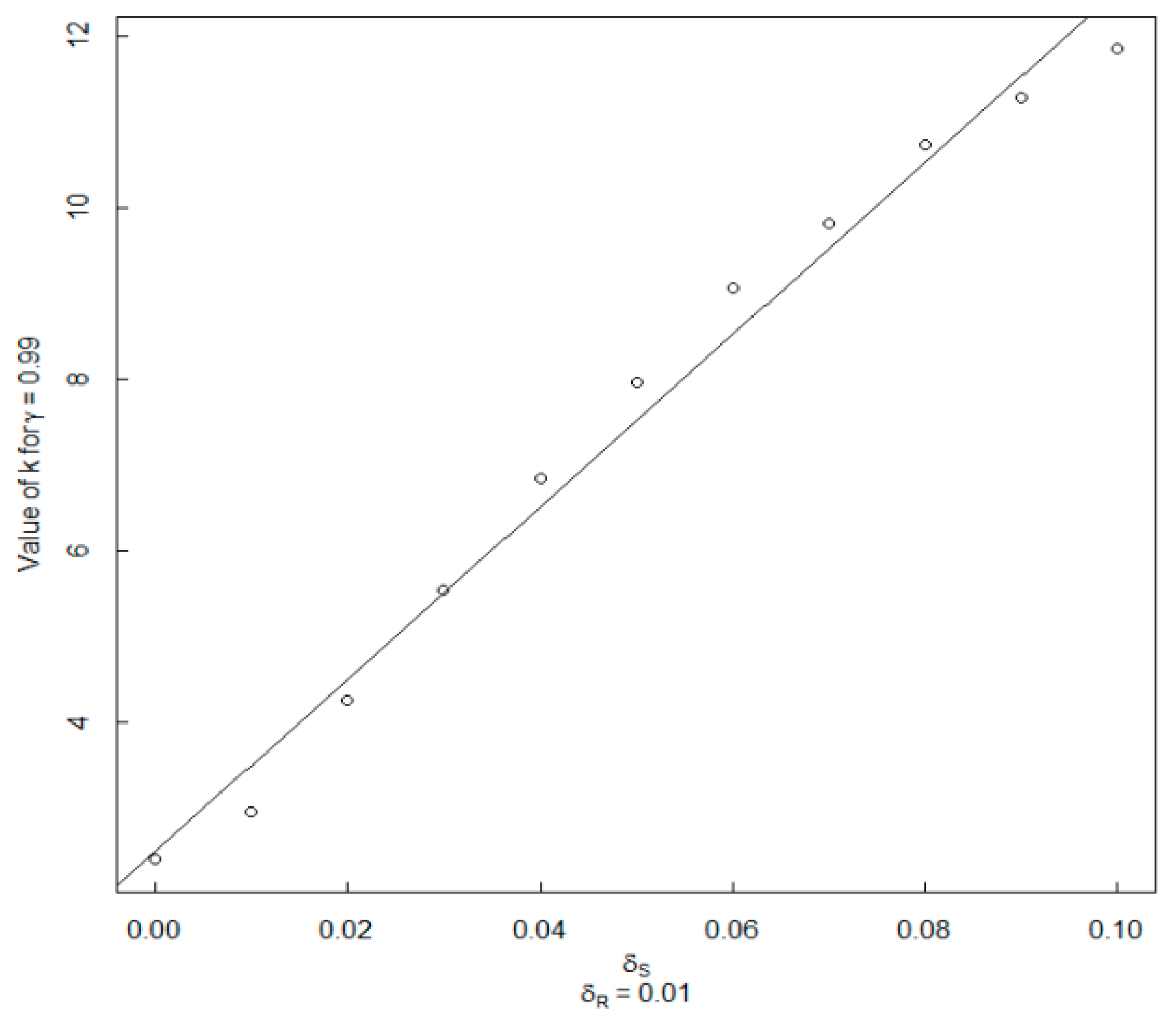
For g = 3 and n = 10, and ${\delta }_R=0.01,$ Figure 3 plots the required value of k versus ${\delta }_S$, such that $P(d\ge k{\widehat{\delta }}_T)\le 0.05$, with probability of at least $p=0.99$.

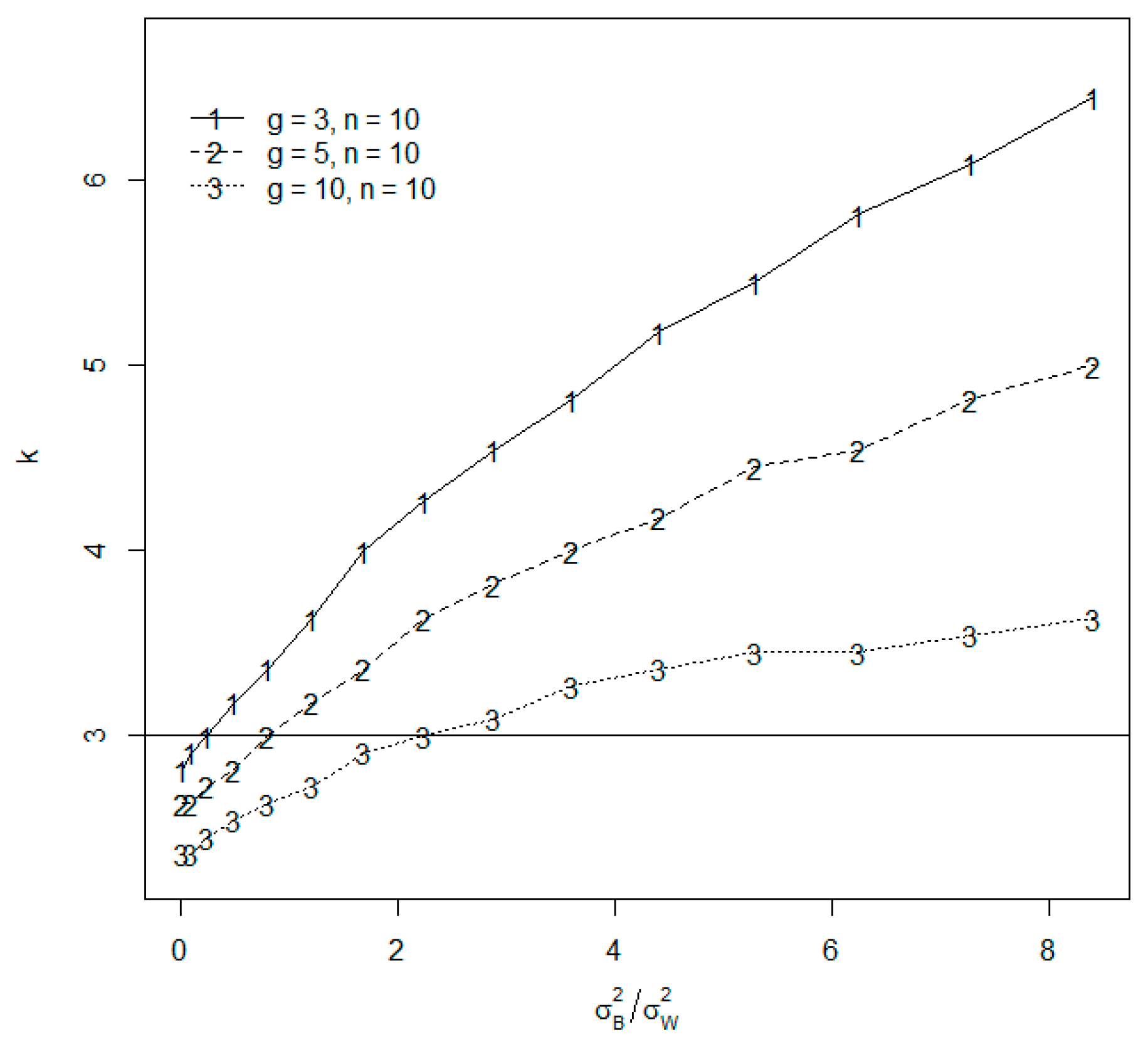
Figure 4 plots the required value of k for g = 3, 5, or 10, and n = 10 versus $\tau =\frac{{\sigma }_B^2}{{\sigma }_W^2}$. Note that the required value of k increases quite substantially as $\tau =\frac{{\sigma }_B^2}{{\sigma }_W^2}$ increases.

For the data in Figure 1, for a two-sided interval expressed as $0\pm k{\widehat{\sigma }}_T$, if one assumes (correctly) that $\tau =1,$ then the option 2 estimate is $k=2.34$, if the weighted least squares option that is described above is used. If the weighted least squares option is not used, but usual ANOVA estimation is used, then $k=2.92$.

4.1.2. Bayesian Approach

Bayesian ANOVA, such as the one applied to data generated from Equation (3), has been well studied [15,24]; however, Bayesian ANOVA using approximate Bayesian computation (ABC) has not been well studied. ABC has some robustness in misspecifying the true probability distribution for the data, so it is the Bayesian choice that is evaluated here [17,18].

In any Bayesian approach, prior information regarding the magnitudes and/or relative magnitudes of ${\delta }_R^2$ and ${\delta }_S^2$ can be provided. If the prior is “conjugate” for the likelihood, then the posterior is in the same likelihood family as the prior, in which case analytical methods are available to compute posterior prediction intervals for quantities of interest. As a wide variety of priors and likelihoods can be accommodated, modern Bayesian methods do not rely on conjugate priors, but they use numerical methods to obtain samples of ${\delta }_R^2$ and ${\delta }_S^2$ from their approximate posterior distributions [24]. For numerical methods, such as Markov Chain Monte Carlo [23], the user specifies a prior distribution for ${\delta }_R^2$ and ${\delta }_S^2$ and a likelihood (which need not be normal). ABC does not require a likelihood for the data (and, as in any Bayesian approach, ABC accommodates the constraints on variances through prior distributions [17,18,25,26,27,28,29].

The “output” of any Bayesian analysis is the posterior distribution for each model parameter, and so the output of ABC for data generated from Equation (3) is an estimate of the posterior distributions of ${\delta }_R^2$ and ${\delta }_S^2$. No matter what type of Bayesian approach is used, a well-calibrated Bayesian approach satisfies several requirements. One requirement is that, in repeated applications of ABC, approximately 95% of the middle 95% of the posterior distribution for each ${\delta }_R^2$ and ${\delta }_S^2$ should contain the respective true values. That is, the actual coverage should be closely approximated by the nominal coverage. A second requirement is that the true mean squared error (MSE) of the ABC-based estimates of ${\delta }_R^2$ and ${\delta }_S^2$ should be closely approximated by the variance of the ABC-based posterior distributions of ${\delta }_R^2$ and ${\delta }_S^2$. Inference using ABC can be briefly summarized, as follows:

ABC Inference For i in 1, 2, …, N, do these 3 steps: (1) Sample $\theta$ from the prior, $\theta ~f_{\mathrm{prior}}(\theta )$. (2) Simulate data $x^{\prime }$ from the model $x^{\prime }~P(x|\theta )$ (3) Denote the real data as x. If the distance $d(S(x^{\prime }),S(x))\le \epsilon ,\mathrm{accept}\theta {\mathrm{as}\mathrm{an}\mathrm{observation}\mathrm{from}\mathrm{f}}_{\mathrm{posterior}}(\theta |x).$

Experience with ABC suggests that the ABC approximation to ${\mathrm{f}}_{\mathrm{posterior}}(\theta |x)$ improves if step (3) is modified to include a weighting factor, so that trial values of θ simulated from $f_{prior}\left(\theta \right)$ that lead to very small distance $d\left(S\left(x^{\prime }\right),S\left(x\right)\right)$ are more heavily weighted in the estimated posterior [27,28,29].

In ABC, the model has input parameters θ and outputs data x(θ), and there is corresponding real data x_bs. For example, the model could be Equation (3), which specifies how to generate synthetic d data (denoted x here), and it does provide a likelihood; however, the true likelihood that is used to generate the data need not be known to the user. Synthetic data is generated from the model for many trial values of θ, and trial θ values are accepted as contributing to the estimated posterior distribution for θ| x_obs if the distance $d(x_{obs},x(\theta ))$ between $x_{obs}$ and $x(\theta )$ is reasonably small. Alternatively, it is necessary to reduce the dimension of x_obs to a small set of summary statistics S and accept trial values of θ if $d(S\left(x_{obs}\right),S(x(\theta ))<\epsilon$, where $\epsilon$ is a user-chosen threshold, for most applications. Here, for example, $x_{obs}=d=(O-I)/O$ data in each inspection group, and (x_obs) includes the within and between groups sums of squares. Specifically, the ANOVA-based estimator of ${\delta }_R^2$ in Equation (3) is ${\widehat{\delta }}_R^2=\frac{1}{n-g}\{{\displaystyle \sum _{j=1}^g{\displaystyle \sum }_{k=1}^n{(d_{jk}-{\overline{d}}_j)}^2}\}$, and the usual estimate of ${\delta }_S^2$ is ${\widehat{\delta }}_S^2=\frac{{\displaystyle \sum _{j=1}^g({\overline{d}}_j}-\overline{\overline{d}}{)}^2}{g-1}-\frac{{\widehat{\delta }}_R^2}{n}$. Therefore, the quantities ${\widehat{\delta }}_R^2$ and ${\widehat{\delta }}_S^2$ are good choices for the summary statistics for ABC. Recall that, because trial values of θ are accepted if $d(S\left(x_{obs}\right),S(x(\theta ))<\epsilon$, an approximation error to the posterior distribution arises that several ABC options attempt to mitigate. Additionally, recall that such options weight the accepted θ values by the actual distance d(S(x_obs), S(x(θ)) (abctools package in R [20]).

To summarize, ABC applied to data following Equation (3) consists of three steps: (1) sample parameter values of ${\delta }_R^2$ and ${\delta }_S^2$ from their prior distribution p_prior(θ); (2) for each simulated value of θ in (1), simulate data from Equation (2); and, (3) accept a fraction of the sampled prior values in (1) by checking whether the summary statistics that are computed from the data in (2) satisfy $d(S\left(x_{obs}\right),S(x(\theta ))<\epsilon .$ If desired, aiming to improve the approximation to the posterior, adjust the accepted θ values on the basis of the actual $d(S\left(x_{obs}\right),S(x(\theta ))$ value. ABC requires the user to make three choices: the summary statistics, the threshold $\epsilon$, and the measure of distance d. Reference [25] introduced a method to choose the summary statistics that uses the estimated posterior means of the parameters based on pilot simulation runs. Reference [25] used an estimate of the change in posterior p_posterior(θ), when a candidate summary statistic is added to the current set of summary statistics. Reference [26] illustrated a method to evaluate whether a candidate set of summary statistics leads to a well-calibrated posterior, in the same sense that is used in this paper; that is, nominal posterior probability intervals should have approximately the same actual coverage probability, and the posterior variance should agree with the observed MSE in testing.

Note that any Bayesian method can be regarded as approximate, because one almost never knows the exact prior probability distribution. However, from Section 2, $S_W^2$ and $S_B^2$ contain useful information regarding ${\delta }_R^2$ and ${\delta }_S^2$, so this paper’s ABC implementation uses $S_W^2$ and $S_B^2$ as summary statistics. There is also the need to choose the threshold $\epsilon$, which can be done by a grid search to find suitable small $\epsilon$, using two assessments to check whether the approximate posterior is sufficiently accurate. First, the quantiles of the estimated posterior should approximately provide the nominal coverage, which is analogous to the frequentist assessment that, for example, approximately 95% of 95% confidence intervals should contain the true parameter. Second, the estimated MSE (which is the variance of the posterior) should be approximately the actual MSE. In all cases considered here, ABC performs well on the two assessments, with actual coverage and MSE within 1% relative of the nominal coverage and MSE. Furthermore, ABC exhibits modest robustness, still exhibiting good agreement between nominal and actual coverage (and MSME), for example, by replacing the Gaussian with a t distribution with small degrees of freedom, such as five-degrees of freedom. As with any Bayesian method, sensitivity to the assumed prior can be an important topic; the results reported below assumed either a uniform prior (0, 0.20) on ${\delta }_R$ and ${\delta }_S$, but the results are very similar for other moderately-wide priors, such as a gamma prior with appropriate parameters.

As in the frequentist option (Section 4.1.1), for the data in Figure 1, for a two-sided interval expressed as $0\pm k{\widehat{\sigma }}_T$, if one assumes (correctly) that $\tau =1,$ then with $p=0.99$ for $\alpha =0.05$, the ABC estimate of k is $k=3.22$ if the weighted least squares option that is described in Section 4.1.1 is used, or $k=3.60$ if it is not used. Note that these values of $k$ are not directly comparable to the frequentist values of $k$ (2.34, and 2.92, respectively, in Section 4.1.1), because the Bayesian estimate of ${\sigma }_T$ behaves differently from the frequentist estimate of ${\sigma }_T.$

4.2. Approximate Tolerance Interval If ${\sigma }_S^2/{\sigma }_R^2$ Is Unknown

In nearly all applications, ${\sigma }_S^2/{\sigma }_R^2$ is unknown, and the resulting tolerance interval width is considerably larger than if ${\sigma }_S^2/{\sigma }_R^2$ were known. As the tolerance interval width depends on the unknown ${\sigma }_S^2/{\sigma }_R^2$, all of the methods are approximate [4,5,6,7,8,9,10,11,23], including those that are based on simulation.

4.2.1. Frequentist Approach

There are several published approximate TI construction methods if ${\sigma }_S^2/{\sigma }_R^2$ is unknown. Option 1 is to first construct a CI for ${\sigma }_S^2/{\sigma }_R^2$ and then assume some upper value for the true unknown ${\sigma }_S^2/{\sigma }_R^2$. Option 2 uses a generalized confidence interval, which leads to an approximation that is based on the non-central t distribution, as in [8,9]. Option 3 uses a bootstrap adjustment to a conservative approximation [5]. Option 4 uses generalized pivot quantities [7]. Option 5 uses variance recover estimation [6]. There are more approximations; not all are reviewed here, but see [9] for a partial review.

Reference [10] suggests to first construct a CI for $\tau$, and then assumes that $\tau$ is known, set to an upper quantile of the CI (or prediction interval if using ABC). An interval that bounds $\tau$ with high confidence can be easily constructed [15]. However, the CI for $\tau$ can be prohibitively wide in this context, extending from 0.036 to 176 for the data in Figure 1. For option 1, in the inspector verification data example, it is reasonable to assume an upper limit for ${\sigma }_S^2/{\sigma }_R^2$, so large values in a CI for ${\sigma }_S^2/{\sigma }_R^2$ can be excluded from consideration. The largest feasible value for ${\sigma }_S^2/{\sigma }_R^2$ (based on assumption or on a CI) is then used exactly, as in the case where ${\sigma }_S^2/{\sigma }_R^2$ is known.

The approximation for options 2–5 are given in [4,5,6,7,8,9,10,11]. For example, option 2 from [8,9] is $\overline{x}+t_{g-1}(p,\eta )\sqrt{SSB/(g(g-1)n)},$ where $\eta =z_{1-\alpha }\sqrt{(g+(g-1)F_{g-1,g(n-1)}(1-p))SSE/SSB}$.

In the verification data example, it is reasonable to assume that $\mu =0$, so the term $\overline{x}$ is not needed in the approximation or in corresponding simulations. For the data in Figure 1, for a two-sided interval expressed as $0\pm k{\widehat{\sigma }}_T$, not knowing $\tau$ leads to a much larger value, k = 11.2 for 99% confidence in 95% coverage. For 95% confidence in 90% coverage, k = 4.2.

Regarding the accuracy of the approximation, options 2–5 are reasonably accurate for Gaussian data, with each option being better or worse than other options in some regions of the parameter space. For example, option 2 has nearly 0.99 actual frequency (with a nominal frequency also of 0.99) of containing $1-\alpha$ percent of the d values for $\tau =\frac{{\delta }_B^2}{{\delta }_W^2}$ near 1. However, if $\tau$ is close to zero, then option 2 can have much lower actual frequency, such as 0.7 for $\tau$ = 0.01.

4.2.2. Bayesian Approach

To illustrate ABC, Figure 5 plots the estimated posterior assuming that either $\tau =\frac{{\delta }_B^2}{{\delta }_W^2}=\frac{{\sigma }_B^2}{{\sigma }_W^2}$ is known or unknown, for a uniform prior on ${\delta }_T$ (from 0 to 0.20) with n = 10, g =5, and data simulated from Equation (3) using ${\delta }_S={\delta }_R=0.01.$ The two diagnostic assessments indicate that the ABC-based posterior distributions are adequate approximations.

For the data in Figure 1, for a two-sided interval expressed as $0\pm k{\widehat{\sigma }}_T$, a probability interval using ABC that bounds $\tau$ with probability p = 0.99 ranges from 0.06 to 4.5 for the data in Figure 1. This probability interval is much narrower than the wide CI that is given in Section 4.2.1 in the frequentist approach (0.036 to 176), because a somewhat narrow prior was assumed, with a maximum assumed value of $\tau =4$, leading to $0\pm 5.2{\widehat{\sigma }}_T$ (refer to Figure 4 for g = 3, n = 10 with $\tau =4.5$).

5. Semi-Parametric Approach

A semiparametric approach lies between the parametric and nonparametric extremes. For example, one semiparametric option is bspmma (which uses a dirichlet process prior) that can be compared to the parametric case, and for a two-sided interval expressed as $0\pm k{\widehat{\sigma }}_T$, requires k = 4.2 for the data in Figure 1. The R code bspmma [12] can be used in one-way random effects ANOVA to estimate the posterior distribution of S. The acronym bspmma stands for Bayesian semiparametric models for meta-analysis [12], and the R code uses model selection that is based on the Radon–Nikodym derivative (a key concept in measure theory). The posterior distribution of R can be obtained by any of several common approaches. The k = 4.2 result for the S + R distribution used a parametric bootstrap [30], in which sample i from the posterior distribution of S + R used bspmma to generate the S value and from $N(0,{\widehat{\sigma }}_{R_i})$ to generate the R value. The standard deviation ${\widehat{\sigma }}_{R_i}$ is sampled from the posterior distribution of ${\sigma }_{R_i}$.

The semi-parametric approach that was used in this context assumes that R has a normal distribution and S has an arbitrary (unknown) distribution. Interestingly, in this case, the covariance between MSB and MSW is 0, because $\mathrm{cov}(MSB,MSW)=\frac{{\mu }_{4,R}-3{\sigma }_R^4}{ng},$ where ${\mu }_{4,R}$ is the fourth central moment, ${\mu }_{4,R}=E(R^4)$, and then because ${\mu }_{4,R}=3{\sigma }_R^4$ for a normal distribution [15], $\mathrm{cov}(MSB,MSW)$ = 0

6. Non-Parametric Approach

The nonparametric approach requires one or more observations from each of the 130 groups (inspection periods), which are far too many groups and observations to be practical. The basis for the nonparametric result of n = 130 is an application of order statistics [13], and the expression for the required sample size n from the S + R distribution in model 2 is $1-n{p}^{n-1}+(n-1)p^n$, where p is the desired probability. If the requirement is 95% probability that the tolerance interval that is based on that the interval $X_{(n)}-X_{(1)}=\max -\min$ contains at least 95% of future values, then n = 93. Raising the requirement from 95% probability to 99% probability increases the required n to n = 130, as given.

7. Summary

This paper reviewed TI-based options to set alarm thresholds in random effects one-way ANOVA, using an example that involves inspector verification in which the inspections are the groups. In the example, within-group variance is random measurement error variance; between-group variance is systematic measurement error variance. There are no exact TI methods for two-sided testing in such data, even if both the random and systematic components are Gaussian.

Although the current practice of using $0\pm 3{\widehat{\delta }}_T$ has acceptably small FAP for a modest number of groups and observations per group, the main purpose of this review paper is to investigate when more formal TI-based methods might be preferred. Semi- and non-parametric options were also investigated. Future work will consider TI-based options when the metrology groups must be inferred from data, as in [31].

References

1. Bonner, E.; Burr, T.; Guzzardo, T.; Norman, C.; Zhao, K.; Beddingfield, D.; Geist, W.; Laughter, M.; Lee, T. Ensuring the effectiveness of safeguards through comprehensive uncertainty quantification. J. Nucl. Mater. Manag. 2016, 44, 53–61. [Google Scholar]
2. Walsh, S.; Burr, T.; Martin, K. The IAEA error approach to variance estimation for use in material balance evaluation and the international target values, and comparison to metrological definitions of precision. J. Nucl. Mater. Manag. 2017, 45, 4–14. [Google Scholar]
3. Burr, T.; Krieger, T.; Norman, C.; Zhao, K. The impact of metrology study sample size on verification samples calculations in IAEA safeguards. Eur. J. Nucl. Sci. Technol. 2016, 2, 36. [Google Scholar]
4. Young, D. Tolerance: An R package for estimating tolerance intervals. J. Stat. Softw. 2010, 36, 1–39. [Google Scholar] [CrossRef]
5. Zou, G.; Donner, A. Construction of confidence limits about effect measures: A general approach. Stat. Med. 2008, 27, 1693–1702. [Google Scholar] [CrossRef]
6. Hoffman, D. One-sided tolerance limits for balanced and unbalanced random effects models. Technometrics 2010, 52, 303–312. [Google Scholar] [CrossRef]
7. Liao, C.; Lin, T.; Iyer, H. One- and two-sided tolerance intervals for general balanced mixed models and unbalanced one-way random models. Technometrics 2005, 47, 323–335. [Google Scholar] [CrossRef]
8. Krishnamoorthy, K.; Mathew, T. One-sided tolerance limits in balanced and unbalanced one-way random models based on generalized confidence intervals. Technometrics 2004, 46, 44–52. [Google Scholar]
9. Krishnamoorthy, K.; Peng, J. Approximate one-sided tolerance limits in random effects model and in some mixed models and comparisons. J. Stat. Comput. Simul. 2015, 85, 1651–1666. [Google Scholar] [CrossRef]
10. Bhaumik, D.; Kulkarni, P. A simple and exact method of constructing tolerance intervals for the one-way ANOVA with random effects. Am. Stat. 1996, 50, 31–323. [Google Scholar]
11. Kraemer, K. Confidence Interval for Variance Components and Functions of Variance Components in the Random Effects Model under Non-Normality. Ph.D. Thesis, Iowa State University, Ames, IA, USA, 2012. [Google Scholar]
12. Burr, D. bspmma: An R package for Bayesian semiparametric models for meta-analysis. J. Stat. Softw. 2012, 50, 1–23. [Google Scholar] [CrossRef]
13. Hogg, R.; Craig, A. Introduction to Mathematical Statistics, 4th ed.; Macmmillan: New York, NY, USA, 1978. [Google Scholar]
14. Burr, T.; Knepper, P. A study of the effect of measurement error in predictor variables in nondestructive assay. Appl. Radiat. Isot. 2000, 53, 547–555. [Google Scholar] [CrossRef]
15. Miller, R. Beyond ANOVA: Basics of Applied Statistics; Chapman & Hall: Boca Raton, FL, USA, 1998. [Google Scholar]
16. Martin, K.; Böckenhoff, A. Analysis of short-term systematic measurement error variance for the difference of paired data without repetition of measurement. Adv. Stat. Anal. 2007, 91, 291–310. [Google Scholar] [CrossRef]
17. Burr, T.; Croft, S.; Krieger, T.; Martin, K.; Norman, C.; Walsh, S. Uncertainty quantification for radiation measurements: Bottom-up error variance estimation using calibration information. Appl. Radiat. Isot. 2015, 108, 49–57. [Google Scholar] [CrossRef] [PubMed]
18. Burr, T.; Croft, S.; Jarman, K.; Nicholson, A.; Norman, C.; Walsh, S. Improved uncertainty quantification in nondestructive assay for nonproliferation. Chemometrics 2016, 159, 164–173. [Google Scholar]
19. Zhao, K.; Penkin, P.; Norman, C.; Balsely, S.; Mayer, K.; Peerani, P.; Pietri, P.; Tapodi, S.; Tsutaki, Y.; Boella, M.; et al. STR-368 International target values 2010 for measurement uncertainties in safeguarding nuclear materials, IAEA, Vienna. 2010. Available online: www.inmm.org (accessed on 17 December 2017).
20. R Core Team. R: A Language and Environment for Statistical Computing; R Foundation for Statistical Computing: Vienna, Austria, 2012; ISBN 3-900051-07-0. Available online: http://www.R-project.org (accessed on 17 February 2015).
21. Marsaglia, G. Ratios of normal variables. J. Stat. Softw. 2006, 16, 2. [Google Scholar] [CrossRef]
22. Hamada, M.; Johnson, V.; Moore, L.; Wendelberger, J. Bayesian prediction intervals and their relation to tolerance intervals. Technometrics 2004, 46, 452–459. [Google Scholar] [CrossRef]
23. Agboraw, E.; Bonner, E.; Burr, T.; Croft, S.; Kirkpatrick, J.; Krieger, T.; Norman, C.; Santi, P. Revisiting Currie’s minimum detectable activity for nondestructive assay by gamma detection using tolerance intervals. Esarda Bull. 2017, 54, 14–22. [Google Scholar]
24. Carlin, B.; John, B.; Stern, H.; Rubin, D. Bayesian Data Analysis, 1st ed.; Chapman and Hall: Boca Raton, FL, USA, 1995. [Google Scholar]
25. Fearnhead, P.; Prangle, D. Constructing summary statistics for approximate Bayesian computation: Semi-automatic approximate Bayesian computation. J. R. Stat. Soc. B 2012, 74, 419–474. [Google Scholar] [CrossRef]
26. Joyce, P.; Marjoram, P. Approximately sufficient statistics and Bayesian computation. Stat. Appl. Genet. Mol. Biol. 2008, 7, 26. [Google Scholar] [CrossRef] [PubMed]
27. Burr, T.; Skurikhin, A. Selecting summary statistics in approximate Bayesian computation for calibrating stochastic models. Biomed. Res. Int. 2013, 2013, 210646. [Google Scholar] [CrossRef] [PubMed]
28. Blum, M.; Nunes, M.; Prangle, D.; Sisson, S. A comparative review of dimension reduction methods in approximate Bayesian computation. Stat. Sci. 2013, 28, 189–208. [Google Scholar] [CrossRef]
29. Nunes, M.; Prangle, D. abctools: An R package for tuning approximate Bayesian computation analyses. R. J. 2016, 7, 189–205. [Google Scholar] [CrossRef]
30. Efron, B.; Hastie, T. Computer Age Statistical Inference; Cambridge University Press: Cambridge, UK, 2016. [Google Scholar]
31. Burr, T.; Martin, K.; Norman, C.; Zhao, K. Analysis of variance for item differences in verification data with unknown groups. Sci. Technol. Nucl. Install. 2019, 2019, 1769149. [Google Scholar] [CrossRef]
Figure 1. Simulated verification measurement data with δ S = δ R = 0.01 . The relative difference d = ( o i ) / o is plotted for each of 10 paired (o,i) measurements in each of three groups, for a total of 30 relative differences. The mean relative difference within each group (inspection period) is indicated by a horizontal line through the respective group means of the paired relative differences. The 3 sets of 10 d values (multiplied by 100 for ease of reading) are {(−0.52, 1.72, −0.66, −0.15, −0.06, 0.35, 1.70, −0.35, −0.17, 2.35), (−1.14, −2.38,0.40, −1.12, −1.36, −1.28, −1.67, 0.52 −1.65, −0.03), (−1.12, −1.04, −0.63, −1.19, 0.19, −1.63, 0.07, −0.34, −1.43, −1.50)}.
Stats 02 00020 g001
Figure 2. Example with n = 5 real d = o i o values in each of the four inspection periods.
Stats 02 00020 g002
Figure 3. The value of k needed such that P ( d k δ ^ T ) 0.05 , with probability at least p = 0.99 versus δ S for δ R = 0.01 .
Stats 02 00020 g003
Figure 4. The required value of k for g = 3, 5, or 10, and n = 10 versus τ = σ B 2 σ W 2 .
Stats 02 00020 g004
Figure 5. The estimated pdf for when τ 2 = δ B 2 δ W 2 is known and unknown.
Stats 02 00020 g005