Historical Global Review of Acid-Volatile Sulfide Sediment Monitoring Data

Lenwood W. Hall, Jr.; Ronald D. Anderson

doi:10.3390/soilsystems6030071

and

Wye Research and Education Center, Agricultural Experiment Station, College of Agriculture and Natural Resources, University of Maryland, Queenstown, MD 21658, USA

^*

Author to whom correspondence should be addressed.

Soil Syst.2022, 6(3), 71;https://doi.org/10.3390/soilsystems6030071

This article belongs to the Special Issue Emerging Contaminants in Soil and Water: Sources, Behaviour, and Environmental and Human Health Risks

Version Notes

Order Reprints

Abstract

Acid-volatile sulfides (AVS) are strongly associated with the bioavailability of some divalent metals such as cadmium, copper, lead, nickel and zinc. However, the global spatial variability of AVS for aquatic systems is unknown. The specific goals of this study were to: (1) summarize all available AVS monitoring data from all types of freshwater and saltwater waterbodies (streams/creeks, rivers, lakes/ponds/reservoirs and estuarine/marine areas) and (2) compare AVS concentrations from these various types of waterbodies considering both soil type classification and biomes. AVS measurements were reported from 21 different countries. A total of 17 different soil types were reported for all waterbody types and both podzols and luvisols were found in all waterbody types. Nine different biomes were sampled for all waterbody types. The temperate broadleaf and mixed forest biome was sampled for AVS in all waterbody types. Mean AVS concentrations ranged from 0.01 to 503 µmoles/g for 140 different waterbody types and the 90th centile for all these waterbodies was 49.4 µmoles/g. A ranking of waterbody type means from low to high AVS measurements showed the lowest mean value was reported for streams/creeks (5.12 µmoles/g; range from 0.1 to 39.8 µmoles/g) followed by lakes/ponds/reservoirs (11.3 µmoles/g; range from 0.79 to 127 µmoles/g); estuarine/marine areas (27.2 µmoles/g; range from 0.06 to 503 µmoles/g) and rivers (27.7 µmoles/g; range from 1.13 to 197 µmoles/g). The data provided in this study are compelling as it showed that the high variability of AVS measurements within each waterbody type as well as the variability of AVS within specific locations were often multiple orders of magnitude differences for concentration ranges. Therefore, a comprehensive spatial and temporal scale sampling of AVS in concert with divalent metals analysis is critical to avoid possible errors when evaluating the potential ecological risk of divalent metals in sediment.

Keywords:

acid-volatile sulfides; divalent metals; bioavailability; soil types; biomes

1. Introduction

Acid-volatile sulfides (AVS) are defined as the sulfides that are evolved and collected from sediments when treated with hydrochloric acid [1]. AVS are considered to be complex and variable components represented by varying groups of sulfur components [2]. AVS in sediment have been reported to be strongly associated with the bioavailabilty of some divalent metals such cadmium, copper, lead, nickel and zinc [3,4]. Sediment is likely non-toxic if the concentration of AVS exceeds concentrations of simultaneously extracted metals (SEM), but if concentrations of SEM exceed AVS, the sediment may or may not be toxic [3,4]. Therefore, accurate and representative measurements of AVS in sediment are critical for any ecological risk assessment for single or multiple divalent metals because this allows the bioavailable fraction is determined.

AVS levels are controlled by many correlated biological, geological, chemical and hydrological factors. Microbial decomposition of organic matter and various mineral phases are responsible for AVS in sediments [2,5]. Microhabitat and nutrient characteristics impact the colonization of microfauna that are responsible for subsurface reductions in sulfates [1]. Ulrich et al. [6] reported that microfauna prefer sandy substrate interbedded with organic rich sediment such as clay. Microbial sulfate reduction occurs because sand particles provide the preferred substrate physical habitat, and an organic rich interface provides nutrient stimulation.

Regional bed rock lithology along with parent soil material are also important factors influencing the presence and abundance of AVS in the sediment of aquatic ecosystems. Sulfur is widely distributed as native deposits near volcanoes and hot springs and is a component of sulphide minerals such as galena, pyrite and sphalerite and is also found in meteorites [7]. Significant deposits exist in salt domes along the Gulf Coast of the USA and in large evaporate deposits in eastern Europe and western Asia. Gray and Murphy [8] have reported low concentrations of sulfur in igneous soils due to gas-phase loss from these elements in magma.

Chemical factors such as anoxic organic rich sediments from fine grain depositional areas can result in higher concentrations of AVS in the aquatic environment [9]. In contrast, lower AVS concentrations are found in oxic sediments with low concentrations of organic matter. Seasonally related temperature, which influences organic matter degradation, is also a key parameter impacting AVS concentrations in sediment [10]. Leonard et al. [11] have reported that AVS concentrations in lake sediments are directly correlated with the temperature of the overlying lake water. Other investigators have also reported large fluctuations in the sediment concentrations of AVS in lakes with a seasonally anoxic hypolimnion [12].

Hydrological factors such as stream flow can also be a factor in determining ambient concentrations of AVS as low-flow low-gradient waterbodies with high organic matter dominated by depositional areas would be expected to have higher concentrations of AVS [1]. Lower concentrations of AVS would be expected in high gradient streams dominated by oxic sediments with larger grain sediment material.

Griethuysen et al. [13] have reported that there is a lack of data on the spatial variability of AVS for aquatic systems. Therefore, summarizing AVS concentrations from various areas of the world to determine spatial differences is clearly a research need based on the importance of AVS for determining the bioavailability of metals in sediment. The specific goals of this study were to use a literature review approach to: (1) summarize all available AVS data from all types of freshwater and saltwater waterbodies (streams/creeks, rivers, lakes/ponds/reservoirs and estuarine/marine areas); and (2) compare AVS concentrations from these various types of waterbodies considering both soil type classification and biomes.

2. Materials and Methods

AVS studies in the literature with monitoring data were located using a general Google search. Key words used for the search were acid-volatile sulfides, AVS and sediment. There were no date restrictions on the data used. When relevant titles were found, the documents were downloaded directly from journal websites via the University of Maryland Libraries system, which allowed access to journal articles without payment. After the documents were obtained, they were evaluated to determine if AVS measurements were provided either within the document or in supplementary material.

References were reviewed for key information that would be used in the main manuscript historical AVS summary, as shown in Table 1, Table 2, Table 3 and Table 4 as described below. Several of the variables needed for this table such as waterbody type, soil type and biome were dependent on the location of the sample sites. The references were searched for coordinates and/or maps of sample sites as well as any descriptions in the text or direct contacts with the authors of the papers that would help to determine the site locations.

Table 1. Summary of historical acid-volatile sulfides (AVS) sediment data from streams and creeks.

Table 2. Summary of historical acid-volatile sulfides (AVS) sediment data from rivers and canals.

Table 3. Summary of historical acid-volatile sulfides (AVS) sediment data from ponds, lakes and reservoirs.

Table 4. Summary of historical acid-volatile sulfides (AVS) sediment data estuarine and marine waterbodies.

Copies of the relevant raw AVS data were transferred to Excel spreadsheets for later analyses (see Data availability statement). In order to have consistent units for all data analysis, AVS data were provided in µmoles/g.

AVS sediment data were organized by waterbody type for each reference in Table 1, Table 2, Table 3 and Table 4. Waterbody type categories were freshwater streams/creeks (Table 1), rivers (Table 2), lakes/ponds/reservoirs (Table 3) and esturarine/marine areas (Table 4). These four tables contain the following information: (1) location; (2) waterbody type; (3) soil type; (4) biome types; (5) were depositional areas targeted? (6) number of sites sampled and frequency; (7) AVS concentrations in µmoles/g including minimum, maximum and mean values; and (8) reference.

A total of 26 soil types were identified for the various references in Table 1, Table 2, Table 3 and Table 4 [74]. These soil types were as follows: fluvisols, gleysols, regosols, lithosols, arenosols, rendzihas, rankers, andosols, verisols, solonchaks, solonetz, yermosols, xerosols, kastanozems, chernozems, phaeozoms, greyzems, cambisols, luvisols, podzoluvisols, podsols, planosols, acrisols, nitosols, ferralsols and histosols. In some cases, more than one soil type was used for a reference.

A total of 14 biomes were also used for each reference in Table 1, Table 2, Table 3 and Table 4 [75]. Biomes are defined as a biogeographical unit consisting of a biological community that has formed in response to a shared regional climate [76]. The biomes for each reference were as follows: tropical and subtropical moist broadleaf forest; tropical and subtropical dry broadleaf forest; tropical and subtropical coniferous forest; temperate broadleaf and mixed forest; temperate coniferous forest; boreal forest/taiga; tropical and subtropical grasslands, savannas and shrublands; temperate grasslands, savannas, and shrublands; flooded grasslands and savannas; montane grasslands and shrublands; tundra; Mediterranean forest, woodlands and scrub; desert and xeric scrublands; and mangroves.

The AVS data were placed in the following four waterbody categories (Table 1, Table 2, Table 3 and Table 4) for the statistical analysis described below: streams/creeks, rivers, lakes/ponds/reservoirs and estuarine/marine areas. The approximate locations of the various study areas are presented in Figure 1, Figure 2, Figure 3 and Figure 4.

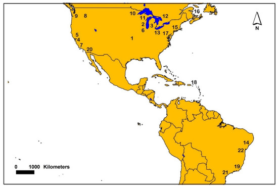
Figure 1. Map showing generalized locations where sediment AVS was sampled from various studies in North and South America. Number symbols on the map are associated with individual or multiple studies and references. The following numbers and associated references are: 1 [14], 2 [15], 3 [16,24], 4 [17,18], 5 [18,21], 6 [19], 7 [20], 8 [24,25,32], 9 [34], 10 [11,15,35,38], 11 [24], 12 [36], 13 [37], 14 [43], 15 [3,44,49], 16 [52], 17 [52,60], 18 [53], 19 [58], 20 [59], 21 [63] and 22 [67].

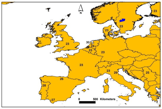
Figure 2. Map showing generalized locations where sediment AVS was sampled from various studies in Europe. Number symbols on the map are associated with individual or multiple studies and references. The following numbers and associated references are: 23 [1], 24 [22,23], 25 [33], 26 [30], 27 [46,47], 28 [61], 29 [64] and 30 [23].

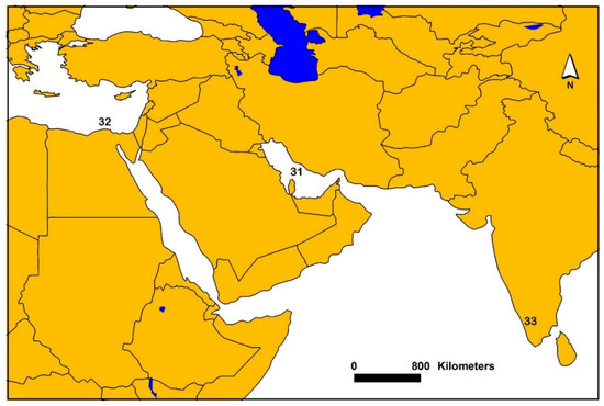
Figure 3. Map showing generalized locations where sediment AVS was sampled from various studies in Egypt, Iran and India. Number symbols on the map are associated with individual or multiple studies and references. The following numbers and associated references are: 31 [45], 32 [62,71] and 33 [66].

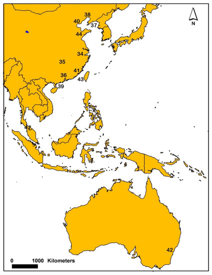
Figure 4. Map showing generalized locations where sediment AVS was sampled from various studies in China and Australia. Number symbols on the map are associated with individual or multiple studies and references. The following numbers and associated references are: 34 [41], 35 [42], 36 [48,50,70], 37 [51], 38 [52], 39 [54], 40 [55], 41 [56,57,69], 42 [65,68], 43 [72] and 44 [51,55,73].

SigmaPlot was used to calculate the AVS mean (with standard deviation), range and 90th centile for each of the four different waterbody type categories of data: streams/creeks, rivers, lakes/ponds/reservoirs and estuarine/marine areas [77]. The AVS concentrations were ranked from low to high and a regression plot was produced with a probability scale on the y axis and a log scale on the x axis (AVS concentration). The a and b factors of the regression equation were used in the following equation to calculate the 90th centile: 10^{(( probit% − (a + 5))/b)} where: probit % = the probit transformed percentage (i.e., if a 90th centile was desired then the probit transformed percentage equal to 90% was used).

3. Results

3.1. General Overview

A total of 120 references containing AVS monitoring data were reviewed (primarily peer-reviewed papers). Sixty-eight of these references were included in Table 1, Table 2, Table 3 and Table 4 along with the descriptive statistics in Table 5. After careful review, 52 of these references were excluded from the tables for any of the following reasons: (1) samples were manipulated in some way (other than homogenization or removal of large debris) before AVS analysis; (2) sulfides were not specifically reported as AVS; (3) sample site locations (coordinates) were not provided; (4) AVS was not reported in µmoles/g; (5) raw data were not provided; (6) AVS was not measured in a natural waterbody and (7) analytical methods for AVS were not provided in the primary document or easily found in supporting references. A summary of the results by waterbody type and in all sites is presented below.

Table 5. Descriptive statistics and centile calculation for five different categories of studies with AVS field data results (µmole/g dry weight).

3.2. Waterbody Types

3.2.1. Streams/Creeks

AVS mean values from 21 streams/creeks ranged from 0.010 to 39.8 µmoles/g as presented in Table 1 and Table 5. The mean of the mean values was 5.12 µmoles/g with a standard deviation of 8.6. The 90th centile for all streams/creeks combined in Table 5 and Figure 5 was 27.2 µmoles/g. There was clearly an outlier value of 0.01 µmoles/g in the 90th centile distribution in Figure 5 that influenced the final 90th centile calculation.

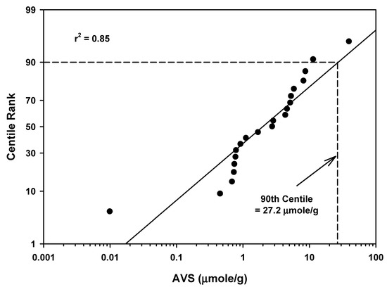
Figure 5. Regression of AVS field study means data for streams/creeks against a probability scale showing the 90th centile rank.

The geographic distribution of AVS measurements in streams/creeks showed that these data were collected in 10 different countries (Table 1; see Figure 1, Figure 2, Figure 3 and Figure 4). Half of these values were reported in the United States. Other countries where AVS measurements were conducted with number of locations sampled were as follows: Netherlands (two), Sweden (one), Denmark (one), England/Wales (one), Finland (one), Belgium (one), France (one), Germany (one) and Italy (one).

A total of nine different soil types were reported in the various streams/creeks sampled for AVS measurements (Table 1). For some locations more than one soil type was reported. The soil types with corresponding number of locations were as follows: luvisols (eleven), cambisols (six), podzols (four), acrisols (two), fluvisols (two), gleysols (one), histosols (one), rendzinas (one) and phaeozems (one). The mean AVS concentrations of 11.7 µmoles/g in streams and creeks were higher in podzols when compared with other soil types, as show in Table 6. The AVS mean concentrations ranged from 3.3 to 6.6 µmoles/g for acrisols, cambisols, luvisols, gleysols and fluvisols. The AVS mean concentrations in histosols, rendzems and phaezems were less than 0.93 µmoles/g.

Table 6. Summary of AVS mean concentrations (µmoles/g) by soil type and waterbody type.

Four different biome types were reported for the streams/creeks where AVS measurements were conducted (Table 1). The most dominant biome reported at 11 locations was the temperate broadleaf and mixed forest biome. The Mediterranean forest woodlands and scrubs biome was found at five locations while the temperate grasslands, savannas and Shrublands biome was found at three locations. The boreal forest/taiga biome was found at one location. The temperate broadleaf and mixed forest biome had the highest AVS mean value of 7.0 µmoles/g followed by the Mediterranean forest woodland and scrub (3.9 µmoles/g), the temperate grasslands, savannas and Shrublands (3.4 µmoles/g) and the boreal forest /tiaga (0.93 µmoles/g) (Table 7).

Table 7. Summary of AVS mean concentrations (µmoles/g) by biome and waterbody type.

Depositional areas were targeted for AVS sampling in streams/creeks in 14 of the 21 locations sampled (Table 1). For the other seven locations, the authors did not provide any information on targeting depositional areas.

3.2.2. Rivers

The AVS mean values ranged from 1.13 to 197 µmoles/g for 16 rivers as presented in Table 2 and Table 5. The mean of the mean values was 27.7 µmoles/g with a standard deviation of 48.7. The 90th centile for all the AVS measurements for rivers was 82.2 µmoles/g (Table 5 and Figure 6). There was one data point (197 µmoles/g) in this distribution that appeared to be an outlier when compared with other values (Figure 6).

Figure 6. Regression of AVS field study means data for rivers against a probability scale showing the 90th centile rank.

AVS measurements for rivers were reported from four different countries (Table 2). Most of the AVS measurements (a total of six) were reported from locations in the United States. The number of locations sampled for other countries were as follows: four locations in Belgium; three locations in the Netherlands, two locations in Serbia and one location in the Netherlands/Belgium.

Eight different soil types were reported for the various AVS measurements in rivers (Table 2). The number of different locations by soil types were as follows: luvisols (eight), fluvisols (seven), podzols (six), podzoluvisols (four), kastanozems (four), regosols (two), chemnozems (two) and phaeozems (one). Both podzols and podzoluvisols were reported to have the highest mean concentrations of AVS in rivers (83.8 µmoles/g) (Table 6). This result was similar to the result from streams discussed above where podsols also had the highest concentrations of AVS. Luvisols were reported to have the second highest concentrations of AVS (35.6 µmoles/g). AVS mean concentrations ranged from 6.6 to 18.2 µmoles/g for kastanozens, fluvisols, regosols, chernozems and phaozems.

For rivers and with AVS measurements, there were three different biome types reported (Table 2). The most dominant biome type found at ten locations was temperate broadleaf and mixed forest. The temperate grasslands, savannas and shrubland biome was found at five locations, while the desert and xeric shrublands biome was found at one location. The highest mean river biome concentration was reported from the temperate broadleaf and mixed forest biome (41.2 µmoles/g) (Table 7). The mean AVS values for the temperate grassland, savanna and shrublands biome (5.5 µmoles/g) and the desert and xeric shrublands biome (4.7 µmoles/g) were similar.

Information on whether the depositional areas were sampled in rivers and with concurrent AVS measurements showed that four of the sixteen locations targeted deposition areas (Table 2). For the other twelve locations, the authors did not provide any information on the sampling depositional areas.

3.2.3. Lakes/Ponds/Reservoirs

The AVS mean values ranged from 0.787 to 127 µmoles/g for 29 lakes, ponds and reservoirs (Table 3 and Table 5). The mean of the mean values was 11.3 µmoles/g with a standard deviation of 23.3. The 90th centile for all the AVS measurements for lakes, ponds and reservoirs was 27.8 µmoles/g (Table 5 and Figure 7). There was one high value in the 90th centile calculation (127 µmoles/g) that appeared to be an outlier when compared with other AVS concentrations (Figure 7).

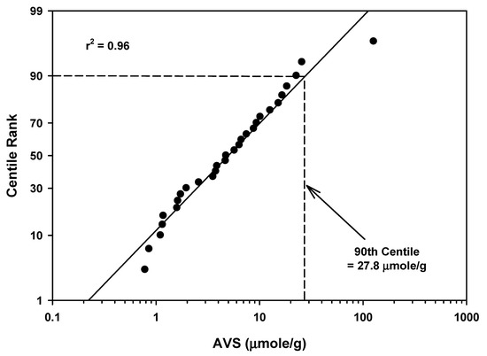
Figure 7. Regression of AVS field study means data for lakes/ponds/reservoirs against a probability scale showing the 90th centile rank.

From a geographic perspective, the AVS data for lakes, ponds and reservoirs were reported from a total of five different countries (Table 3). Most of these lentic sites were located in the United States (18). For the other countries, the number of locations were as follows: Netherlands (four); China (four); Canada (two) and Spain (one).

A total of 10 different soil types were reported for the AVS measurements in lakes, ponds and reservoirs (Table 3). The number of different locations by soil types were as follows: podzols (six), luvisols (five), podzoluvisols (5), histosols (four), cambisols (three), fluvisols (three), gleysols (three), xerosols (one), kastanozems (one) and regosols (one). Histosols, luvisols and podzols had the highest AVS concentrations ranging from 28.3 to 41.9 µmoles/g for lakes, ponds and reservoirs (Table 6). As reported above for both stream/creeks and rivers, podzols had some of the highest, but not the highest, concentrations of AVS values in this waterbody type. The lowest AVS mean concentrations (less than 1.2 µmoles/g) were reported kastanozems and regosols.

There were three different biomes reported for AVS measurements in lakes, ponds and reservoirs (Table 3). The temperate broadleaf and mixed forest biome was reported in twenty-three locations while the temperate grassland, savannas and shrubland biome was reported in five locations and the temperate coniferous forest biome was reported in only one location. The mean AVS measurements by biome were as follows: temperate broadleaf and mixed forest (12.5 µmoles/g), temperate grassland, savannas and shrublands (7.8 µmoles/g) and temperate coniferous forest (1.97 µmoles/g) (Table 7).

For sixteen of the AVS studies conducted in lakes, ponds and reservoirs, the authors did not report any information concerning the sampling of the depositional areas (Table 3). There were two studies where depositional areas were sampled and one study where the authors reported that the depositional areas were clearly not sampled.

3.2.4. Estuarine/Marine Areas

The mean AVS values ranged from 0.058 to 503 µmoles/g for 74 estuarine/marine locations (Table 4 and Table 5). The mean of the mean values was 27.2 µmoles/g with a standard deviation of 67.8. The 90th centile for all the AVS measurements for estuarine/marine areas was 68.2 µmoles/g (Table 5 and Figure 8). There was one high value of 503 µmoles/g that appeared to be an outlier in the 90th centile calculation for estuarine and marine areas (Figure 8).

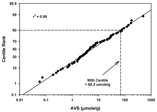
Figure 8. Regression of AVS field study means data for estuarine/marine waterbodies against a probability scale showing the 90th centile rank.

AVS measurements for estuarine/marine areas were reported from thirteen different countries (Table 4). The countries with the greatest number of locations sampled were China (twenty-two locations) and the United States (thirteen locations). The number of locations sampled for the other countries were as follows: Brazil (seven), Egypt (six), Spain (five), Iran (four), Portugal (four), Australia (three), India (three), Tiawan (two), Canada (one) and Italy (one).

A total of 10 different soil types were reported from AVS measurements in estuarine and marine areas (Table 4). The most dominant soil types for the various locations were gleysols (seventeen locations), solonchaks (fifteen locations), cambisols (fifteen locations) and acrisols (fifteen locations). For the other six soil types, the number of different locations were as follows: regosols (twelve locations), polzols (five locations), luvisols (four locations), vertsols (four locations), fluvisols (four locations) and planosoles (one location). The soil types for estuarine and marine areas with the highest mean AVS concentrations were acrisols (99.2 µmoles/g) and podsols (55 µmoles/g) (Table 6). As reported for the other three waterbody types, podsols had some of the highest AVS mean concentrations. Luvisols were reported to have the third highest mean concentrations of AVS (20.1 µmoles/g). For the other seven soil types, the AVS mean concentrations were less than 9.9 µmoles/g.

There were a total of seven different biomes reported for AVS measurements in estuarine and marine areas (Table 4). The temperate broadleaf and mixed forest biome was most dominant as this biome was found in eighteen estuarine and marine locations. The number of locations for the other biomes were as follows: tropical and subtropical moist broadleaf forest (sixteen), Mediterranean forest woodlands and scrub (ten), flooded grasslands and shrublands (eight), mangroves (eight), temperate and coniferous forest (six) and desert and xeric shrublands (five). The highest AVS mean concentration of 164.7 µmoles/g was reported from the temperate and coniferous forest biome (Table 7). Mean AVS concentrations for the other biomes were as follows: mangroves (44.7 µmoles/g), temperate broadleaf and mixed forest (30.9 µmoles/g), Mediterranean forest woodland and scrub (11.8 µmoles/g), flooded grasslands and shrublands (11.1 µmoles/g), tropical and subtropical moist broadleaf forest (7.8 µmoles/g) and desert and xeric shrublands (3.8 µmoles/g).

With the exception of one study [69], there was no information provided by the authors suggesting that depositional areas were targeted for AVS sampling in estuarine/marine areas (Table 4).

3.2.5. All Waterbodies

Mean AVS values ranged from 0.058 to 503 µmoles/g for 140 waterbodies (Table 5). The mean of the mean values was 20.7 µmoles/g with a standard deviation of 53.6. The 90th centile for all AVS measurements for all sites was 49.4 µmoles/g (Table 5 and Figure 9). As reported above for estuarine/marine areas, there appeared to be one high outlier data point (503 µmoles/g) in the all-waterbodies 90th centile calculation in Figure 9. In addition, there also appeared to be a very low AVS value of 0.010 µmoles/g in Figure 9 that could be considered an outliner as previously discussed for streams in Figure 5.

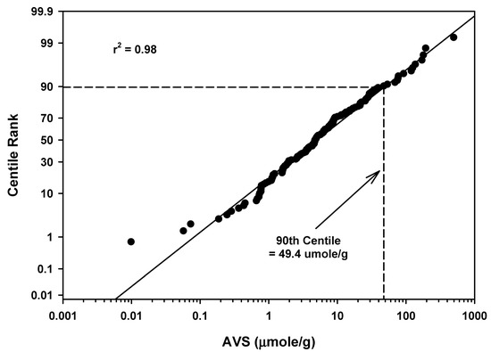
Figure 9. Regression of AVS field study means data for all waterbodies against a probability scale showing the 90th centile rank.

AVS measurements were reported from a total of 21 different countries for all waterbody types as summarized above (Table 1, Table 2, Table 3 and Table 4). The United States was the only country where AVS sampling was conducted in all waterbody types. A total of 17 different soil types were reported for all the waterbody types (Table 1, Table 2, Table 3 and Table 4). Podzols and luvisols were found in all waterbody types. Nine different biomes were sampled for AVS measurements in all waterbodies sampled (Table 1, Table 2, Table 3 and Table 4). The temperate broadleaf and mixed forest biome was sampled for AVS in all waterbody types (Table 1, Table 2, Table 3 and Table 4). In most cases, the authors for the various monitoring studies in all waterbody types did not provide any information on targeting depositional areas for AVS sampling. The exception was streams/creeks where depositional areas were targeted for some of the sites sampled.

4. Discussion

There were a total of 140 locations sampled for AVS for all waterbody types based on this historical review (Table 5). Approximately half of the locations sampled for AVS were located in estuarine/marine areas; therefore, the available data is somewhat skewed for this waterbody type. The numbers of locations sampled for AVS in rivers (only 16 locations) and streams/creeks (only 21 locations) was less than the other two waterbody types. Therefore, additional AVS monitoring in these lotic aquatic systems is recommended.

AVS measurements in 13 different countries were reported for estuarine/marine locations and for streams/creeks AVS measurements were reported in 10 different countries. For rivers and lakes/ponds/reservoirs, AVS data were only available from four to five countries. Most of the AVS data were reported from waters in the United States, although for estuarine/marine areas there were more sites sampled for AVS in China than in the United States. In summary, the geographic extent of AVS data, particularly for rivers and lentic systems (lakes, ponds, reservoirs) is limited and should be expanded to include more countries.

The most dominant soil type generally reported for all waterbody types except the estuarine/marine areas was luvisols. Luvisols are technically characterized by a surface accumulation of humus overlying an extensively leached layer devoid of clay and iron-bearing minerals [78]. Luvisols extend over 500 to 600 million hectares worldwide and are dominant in temperate regions such as west/central Russia, the USA and central Europe as well as the Mediterranean region and southern Australia [78]. Based on the geographic distribution of AVS sampling sites, it is clear that the AVS data base is biased for luvisols. Therefore, the possible relationship of luvisols and AVS becomes important. Based on our analysis, for rivers, lakes/ponds/reservoirs and estuarine/marine areas, luvisol areas have some of the highest concentrations of AVS (Table 6). Naturally occurring sulfur in luvisols may be contributing to the elevated AVS in these waterbodies [79].

The most dominant biome sampled for AVS among all waterbody types was the temperate broadleaf and mixed forest biome. This biome is defined as temperate climate habitat with broadleaf ecoregions with conifer and broadleaf trees mixed in coniferous forest ecoregions [80]. The temperate broadleaf and mixed forest biome is particularly dominant in central China, eastern North America, Caucasus, Himalayas, southern Europe, and the Russian Far East [80]. The temperate broadleaf and mixed forest biome was reported to have the highest concentrations of AVS for streams/creeks, rivers, and lakes/ponds/reservoirs, but for estuarine marine areas the temperate coniferous forest biome had the highest AVS concentrations (Table 7).

AVS is highly variable for all waterbody types combined with mean values ranging from 0.010 to 503 µmoles/g. The variability of AVS within each waterbody type as well as the variability of AVS within specific sampling locations is compelling based on the data provided in this manuscript. For lotic water systems such as streams, the AVS mean values ranged from 0.01 to 39.8 µmoles/g for all streams/creeks (Table 5). This is a 3980 × difference between a low to high concentration. The variability is even more extreme when evaluating site-specific stream data. For example, Burton et al. [1] reported AVS concentrations ranging from 0.02 to 44 µmoles/g for six stream sites sampled in Belgium. This represents a 2200 × difference between low and high values.

The same variability trend was also reported for other lotic water systems such as rivers as the range of mean AVS values reported was 1.13 to 197 µmoles/g for all rivers in Table 5 (174 × difference between low and high value). In a specific river study, De Jong et al. [27] sampled 28 sites in the north Belgium Flanders region and reported lowland river sediment AVS concentrations ranging from 0.004 to 357 µmoles/g (89,250 × difference between low and high values). The variability of AVS measurements in rivers based on this one specific study is even greater than that reported for streams as discussed above.

For lentic aquatic systems such as lakes/ponds/reservoirs, AVS mean concentrations ranged from 0.787 to 127 µmoles/g (161 × difference between low and high values) (Table 5). This is a similar value reported above for all rivers. A specific study by Besser et al. [24] in a Michigan (US) lake showed AVS concentrations ranging from 0.1 to 65 µmoles/g (650 × difference between the low and high value)

Variability of AVS measurements is also well documented for estuarine/marine areas that may be subjected to tidal cycles, with mean AVS values ranging from 0.058 to 503 µmoles/g (8672 × difference between low and high values). A specific study conducted by the Maryland Department of the Environment 2021 in the Middle Harbor Patapsco River estuary showed AVS concentrations ranging from 0.02 to 515.6 µmoles/g (25,780 × difference between low and high value) based on sampling of 14 sites [60].

The variability issue of AVS for all waterbody types reported in this study becomes extremely important when attempting to determine the bioavailability and potential toxicity of divalent metals such as cadmium, copper, lead, nickel and zinc in sediment. Comprehensive representative spatial and temporal scale sampling with concurrent AVS measurements in concert with metals analysis in a waterbody, such as a stream, is therefore critical to avoid possible errors when evaluating the potential ecological risk of metals in sediment. In other words, taking only a few samples from a single waterbody only once could be misleading when attempting to determine the ecological risk of metals due to the high variability of AVS. It is well documented that if the concentration of AVS exceeds the concentrations of SEMs [1], the sediment is likely non-toxic to resident aquatic biota such as benthic invertebrates, so representative sampling to correctly characterize AVS for a waterbody is critical for determining a correct ecological risk decision for metals.

A ranking of waterbody types means from low to high AVS measurements showed the lowest mean value was reported for stream/creeks (5.12 µmoles/g) followed by lakes/ponds/reservoirs (11.3 µmoles/g), estuarine/marine areas (27.2 µmoles/g) and rivers (27.7 µmoles/g) (Table 5). Based on a comparative summary of AVS by waterbody type it appears that streams/creeks may be more vulnerable to divalent metal toxicity because their AVS values were lower when compared with rivers, lakes/ponds/reservoirs and estuarine/marine areas. This does not exclude metal toxicity from these other waterbodies, but SEMs would need to be higher and exceed these higher AVS concentrations in order to be toxic. The lower AVS concentrations in streams/creeks compared with other waterbody types may be related to hydrological factors such as stream flow and the presence of larger grain sediment material [1].

5. Conclusions

Accurate ecological risk assessments of divalent metals such as cadmium, copper, lead, nickel and zinc in sediments are critical for science-based regulatory decisions. The bioavailability of these divalent metals and potential toxicity to resident biota is controlled by the binding capability of AVS. Therefore, the bioavailable fraction of these divalent metals as opposed to their total concentrations is a more accurate prediction of ecological risk. The results from this global summary of AVS data from 21 countries by waterbody type, soil type and biome provide valuable background data on concentration ranges that may be found. AVS monitoring data for flowing waterbodies such streams/creeks and rivers was somewhat limited compared with lentic systems such as lakes, ponds and reservoirs or tidally influenced estuarine/marine areas. Therefore, additional AVS monitoring data for these lotic waterbody types is recommended. The areas with higher AVS concentrations, such as rivers and estuarine/marine areas, would likely be less vulnerable to divalent metal toxicity in sediment compared to areas such as streams where lower AVS concentrations have been reported. The extremely high variability of AVS concentrations reported both within waterbody types and within specific locations (often multiple orders of magnitude differences between the low and high values) highlights the need for extensive spatial and temporal AVS sampling within a waterbody with concurrent metal measurements to accurately assess the ecological risk of divalent metals. Failure to conduct these types of representative field monitoring studies may lead to inaccurate predictions of the divalent metal ecological risk to resident aquatic biota.

Supplementary Materials

The following supporting information can be downloaded at: https://www.mdpi.com/article/10.3390/soilsystems6030071/s1, Table S1: Hall & Anderson (2022) Supplemental Sediment AVS Data.

Author Contributions

Conceptualizations and writing, L.W.H.J.; historical data searches and development of tables and figures, R.D.A. All authors have read and agreed to the published version of the manuscript.

Funding

This research received no external funding.

Institutional Review Board Statement

Not applicable.

Informed Consent Statement

Not applicable.

Data Availability Statement

The data are available as a separate file (Supplementary Materials).

Acknowledgments

Robert Morris is acknowledged for his constructive comments on the draft manuscript. Albaugh is acknowledged for supporting the collection and analysis of data.

Conflicts of Interest

The authors declare no conflict of interest.

References

Burton, G.A.; Green, A.; Baudo, R.; Forbes, V.; Nguyen, L.T.H.; Janssen, C.R.; Kukkonen, J.; Leppanen, M.; Maltby, L.; Soares, A.; et al. Characterizing sediment acid volatile sulfide concentrations in European Streams. Environ. Toxicol. Chem. 2007, 26, 1–12. [Google Scholar] [CrossRef] [PubMed]
Rickard, D.; Morse, J.W. Acid volatile sulfides (AVS). Mar. Chem. 2005, 97, 141–197. [Google Scholar] [CrossRef]
Di Toro, D.M.; Mahony, J.D.; Hansen, D.J.; Scott, K.J.; Hicks, M.B.; Mayr, S.M.; Redmond, M.S. Toxicity of cadmium in sediments: The role of acid volatile sulfide. Environ. Toxicol. Chem. 1990, 9, 1487–1502. [Google Scholar] [CrossRef]
U. S. Environmental Protection Agency. Procedures for the Derivation of Equilibrium Partitioning Sediment Benchmarks (ESBs) for the Protection of Benthic Organism: Metal Mixtures (Cadmium, Copper, Lead, Nickel, Silver, and Zinc); Report EPA/600/R-02/011; Office of Research and Development: Washington, DC, USA, 2005.
Morse, J.W.; Rickard, D. Chemical dynamics of sedimentary acid volatile sulfides. Environ. Sci. Technol. 2004, 38, 131–136. [Google Scholar] [CrossRef] [PubMed]
Ulrich, G.A.; Martino, D.P.; Burger, K.; Routh, J.; Grossman, E.L.; Ammerman, J.W.; Suflita, J.M. Sulfur cycling in the terrestrial subsurface: Commensal interactions, spatial scales, and microbial heterogeneity. Microb. Ecol. 1998, 36, 141–151. [Google Scholar] [CrossRef]
University of Auckland. Geology, Rocks and Minerals. Auckland, New Zealand. 2005. Available online: https://flexiblelearning.aukland.ac.nz/rocks_minerals/minerals/sulfur.html# (accessed on 15 May 2022).
Gray, J.M.; Murphy, B.W. Parent Material and Soils—A Guide to the Influence of Parent Material on Soil Distribution in Eastern Australia; Technical Report 45 (Reprinted 2002); New South Wales Department of Land and Water Conservation: Sydney, WSW, Australia, 1999.
Lander, L.; Reuther, R. Metals in Society and in the Environment: A Critical Review of Current Knowledge on Fluxes, Speciation, Bioavailability and Risk for Adverse Effects of Copper, Chromium, Nickel, and Zinc; Environmental Pollution Series; Kluwer Academic: Dordrecht, The Netherlands, 2004. [Google Scholar]
Van Den Berg, G.A.; Loch, J.P.G.; Van Der Heijdt, L.M.; Zwolsman, J.J.G. Vertical distribution of acid-volatile sulfide and simultaneously extracted metals in a recent sedimentation area of the River Meuse in The Netherlands. Environ. Toxicol. Chem. 1998, 17, 758–763. [Google Scholar] [CrossRef]
Leonard, E.N.; Mattson, V.R.; Benoit, D.A.; Hoke, R.A.; Ankley, G.T. Seasonal variation of acid volatile sulfide concentration in sediment cores from three northeastern Minnesota lakes. Hydrobiologia 1993, 271, 87–95. [Google Scholar] [CrossRef]
Howard, D.E.; Evans, R.D. Acid-volatile sulfide (AVS) in a seasonally anoxic mesotrophic lake: Seasonal and spatial changes in sediment AVS. Environ. Toxicol. Chem. 1993, 12, 1051–1057. [Google Scholar] [CrossRef]
Griethuysen, C.V.; Meijboom, E.W.; Koelmans, A.A. Spatial variation of metals and acid volatile sulfides in floodplain lake sediments. Environ. Toxicol. Chem. 2003, 22, 457–465. [Google Scholar] [CrossRef]
Ankley, G.T.; Liber, K.; Call, D.J.; Markee, T.P.; Canfield, T.J.; Ingersoll, C.G. A field investigation of the relationship between zinc and acid volatile sulfide concentrations in freshwater sediments. J. Aquat. Ecosyst. Health 1996, 5, 255–264. [Google Scholar] [CrossRef]
Carlson, A.R.; Phipps, G.L.; Mattson, V.R. The role of acid-volatile sulfide in determining cadmium bioavailability and toxicity in freshwater sediments. Environ. Toxicol. Chem. 1991, 10, 1309–1319. [Google Scholar] [CrossRef]
Cervi, E.C.; Clark, S.; Boye, K.E.; Gustafsson, J.P.; Baken, S.; Burton, G.A., Jr. Copper transformation, speciation, and detoxification in anoxic and suboxic freshwater sediments. Chemosphere 2021, 282, 131063. [Google Scholar] [CrossRef] [PubMed]
Hall, L.W., Jr.; Killen, W.D.; Anderson, R.D.; Alden, R.W., III. The influence of physical habitat, pyrethroids, and metals on benthic community condition in an urban and residential stream in California. Hum. Ecol. Risk Assess. 2009, 15, 526–553. [Google Scholar] [CrossRef]
Hall, L.W., Jr.; Killen, W.D.; Anderson, R.D.; Alden, R.W., III. A three year assessment of the influence of physical habitat, pyrethroids and metals on benthic communities in two urban California streams. J. Ecosyst. Ecography 2013, 3, 133. [Google Scholar]
Hall, L.W., Jr.; Killen, W.D.; Anderson, R.D.; Alden, R.W., III. The influence of multiple chemical and non-chemical stressors on benthic communities in a mid-west agricultural stream. J. Environ. Sci. Health Part A 2017, 52, 1008–1021. [Google Scholar] [CrossRef]
Hall, L.W., Jr.; Anderson, R.D.; Killen, W.D.; Alden, R.W., III. An analysis of multiple stressors on resident benthic communities in a California agricultural stream. Air Soil Water Res. 2018, 11, 1–18. [Google Scholar] [CrossRef]
Hall, L.W., Jr.; Killen, W.D.; Anderson, R.D.; Alden, R.W., III. Long term bioassessment multiple stressors study in a residential California stream. J. Environ. Sci. Health A 2021, 55, 346–360. [Google Scholar] [CrossRef]
Poot, A.; Meerman, E.; Gillissen, F.; Koelmans, A.A. A kinetic approach to evaluate the association of acid volatile sulfide and simultaneously extracted metals in aquatic sediments. Environ. Toxicol. Chem. 2009, 28, 711–717. [Google Scholar] [CrossRef]
Van Den Hoop, M.A.G.T.; Den Hollander, H.A.; Kerdijk, H.N. Spatial and seasonal variations of acid volatile sulphide (AVS) and simultaneously extracted metals (SEM) in Dutch marine and freshwater sediments. Chemosphere 1997, 35, 2307–2316. [Google Scholar] [CrossRef]
Besser, J.M.; Kubitz, J.A.; Ingersoll, C.G.; Braselton, W.E.; Giesy, J.P. Influences on copper bioaccumulation, growth, and survival of the midge, Chironomus tentans, in metal-contaminated sediments. J. Aquat. Ecosyst. Health 1995, 4, 157–168. [Google Scholar] [CrossRef]
Brumbaugh, W.G.; Ingersoll, C.G.; Kemble, N.E.; May, T.W.; Zajicek, J.L. Chemical characterization of sediments and pore water from the upper Clark Fork River and Milltown Reservoir, Montana. Environ. Toxicol. Chem. 1994, 13, 1971–1983. [Google Scholar] [CrossRef]
De Jonge, M.; Dreesen, F.; De Paepe, J.; Blust, R.; Bervoets, L. Do Acid Volatile Sulfides (AVS) influence the accumulation of sediment-bound metals to benthic invertebrates under natural field conditions? Environ. Sci. Technol. 2009, 43, 4510–4516. [Google Scholar] [CrossRef] [PubMed]
De Jonge, M.; Blust, R.; Bervoets, L. The relation between acid volatile sulfides (AVS) and metal accumulation in aquatic invertebrates: Implications of feeding behavior and ecology. Environ. Pollut. 2010, 158, 1381–1391. [Google Scholar] [CrossRef]
Van Gheluwe, M.; Verdonck, F.; Van Sprang, P. Voluntary risk assessment of copper, copper II sulphate pentahydrate, copper(I)oxide, copper(II)oxide, dicopper chloride trihydroxide, Chapter 3: Environmental effects, Appendix O: Probabilistic assessment of copper bioavailability in sediments. In European Union Risk Assessment Report; European Union: Brussels, Belgium, 2008. [Google Scholar]
Hall, L.W.; Killen, W.D.; Anderson, R.D.; Alden III, R.W. The relationship of benthic community metrics to pyrethroids, metals, and sediment characteristics in Cache Slough, California. J. Environ. Sci. Health A 2015, 51, 154–163. [Google Scholar] [CrossRef] [PubMed]
Méndez-Fernández, L.; De Jonge, M.; Bervoets, L. Influences of sediment geochemistry on metal accumulation rates and toxicity in the aquatic oligochaete Tubifex tubifex. Aquat. Toxicol. 2014, 157, 109–119. [Google Scholar] [CrossRef] [PubMed]
Naylor, C.; Davison, W.; Motelica-Heino, M.; Van Den Berg, G.A.; Van Der Heijdt, L.M. Potential kinetic availability of metals in sulphidic freshwater sediments. Sci. Total Environ. 2006, 357, 208–220. [Google Scholar] [CrossRef]
Patton, G.W.; Crecelius, E.A. Simultaneously Extracted Metals/Acid-Volatile Sulfide and Total Metals in Surface Sediment from the Hanford Reach of the Columbia River and the Lower Snake River; U.S. Department of Energy, Pacific Northwest National Laboratory: Richland, WA, USA, 2001. Available online: http;//www.ntis.gov/ordering (accessed on 15 February 2022).
Prica, M.; Dalmacija, B.; Rončević, S.; Krčmar, D.; Bečelić, M. A comparison of sediment quality results with acid volatile sulfide (AVS) and simultaneously extracted metals (SEM) ratio in Vojvodina (Serbia) sediments. Sci. Total Environ. 2008, 389, 235–244. [Google Scholar] [CrossRef]
Ankley, G.T.; Mattson, V.R.; Leonard, E.N.; West, C.W.; Bennett, J.L. Predicting the acute toxicity of copper in freshwater sediments: Evaluation of the role of acid-volatile sulfide. Environ. Toxicol. Chem. 1993, 12, 315–320. [Google Scholar] [CrossRef]
Allen, H.E.; Fu, G.; Deng, B. Analysis of acid-volatile sulfide (AVS) and simultaneously extracted metals (SEM) for the estimation of potential toxicity in aquatic sediments. Environ. Toxicol. Chem. 1993, 12, 1441–1453. [Google Scholar] [CrossRef]
Huerta-Dlaz, M.A.; Carignan, R.; Tessier, A. Measurement of trace metals associated with acid volatile sulfides and pyrite in organic freshwater sediments. Environ. Sci. Technol. 1993, 27, 2367–2372. [Google Scholar] [CrossRef]
Matisoff, G.; Berton Fisher, J.; McCall, P.L. Kinetics of nutrient and metal release from decomposing lake sediments. Geochim. Cosmochim. Acta 1981, 45, 2333–2347. [Google Scholar] [CrossRef]
Sibley, P.K.; Ankley, G.T.; Cotter, A.M.; Leonard, E.N. Predicting chronic toxicity of sediments spiked with zinc: An evaluation of the acid-volatile sulfide model using a life-cycle test with the midge Chironomus tentans. Environ. Toxicol. Chem. 1996, 15, 2102–2112. [Google Scholar] [CrossRef]
Van Den Berg, G.A.; Buykx, S.E.J.; Van Den Hoop, M.A.G.T.; Van Der Heijdt, L.M.; Zwolsman, J.J.G. Vertical profiles of trace metals and acid-volatile sulphide in a dynamic sedimentary environment: Lake Ketel, The Netherlands. Appl. Geochem. 2001, 16, 781–791. [Google Scholar] [CrossRef]
Van Griethuysen, C.; De Lange, H.J.; Van Den Heuij, M.; De Bies, S.C.; Gillissen, F.; Koelmans, A.A. Temporal dynamics of AVS and SEM in sediment of shallow freshwater floodplain lakes. Appl. Geochem. 2006, 21, 632–642. [Google Scholar] [CrossRef]
Yin, H.B.; Fan, C.X.; Ding, S.M.; Zhang, L.; Li, B. Acid volatile sulfides and simultaneously extracted metals in a metal-polluted area of Taihu Lake, China. Bull. Environ. Contam. Toxicol. 2008, 80, 351–355. [Google Scholar] [CrossRef]
Zheng, L.; Xu, X.Q.; Xie, P. Seasonal and vertical distributions of acid volatile sulfide and metal bioavailability in a shallow, subtropical lake in China. Bull. Environ. Contam. Toxicol. 2004, 72, 326–334. [Google Scholar] [CrossRef]
Alves, J.P.H.; Passos, E.A.; Garcia, C.A.B. Metals and acid volatile sulfide in sediment cores from the Sergipe River Estuary, northeast, Brazil. J. Braz. Chem. Soc. 2007, 18, 748–758. [Google Scholar] [CrossRef]
Ankley, G.T.; Phipps, G.L.; Leonard, E.N.; Benoit, D.A.; Mattson, V.R.; Kosian, P.A.; Cotter, A.M.; Dierkes, J.R.; Hansen, D.J.; Mahony, J.D. Acid-volatile sulfide as a factor mediating cadmium and nickel bioavailability in contaminated sediments. Environ. Toxicol. Chem. 1991, 10, 1299–1307. [Google Scholar] [CrossRef]
Arfaeinia, H.; Nabipour, I.; Ostovar, A.; Asadgol, Z.; Abuee, E.; Keshtkar, M.; Dobaradaran, S. Assessment of sediment quality based on acid-volatile sulfide and simultaneously extracted metals in heavily industrialized area of Asaluyeh, Persian Gulf: Concentrations, spatial distributions, and sediment bioavailability/toxicity. Environ. Sci. Pollut. Res. 2016, 23, 9871–9890. [Google Scholar] [CrossRef]
Campana, O.; Rodríguez, A.; Blasco, J. Bioavailability of heavy metals in the Guadalete River Estuary (SW Iberian Peninsula). Cienc. Mar. 2005, 31, 135–147. [Google Scholar] [CrossRef][Green Version]
Campana, O.; Rodríguez, A.; Blasco, J. Identification of a potential toxic hot spot associated with AVS spatial and seasonal variation. Arch. Environ. Contam. Toxicol. 2009, 56, 416–425. [Google Scholar] [CrossRef] [PubMed]
Chai, M.; Shen, X.; Li, R.; Qiu, G. The risk assessment of heavy metals in Futian mangrove forest sediment in Shenzhen Bay (South China) based on SEM-AVS analysis. Mar. Pollut. Bull. 2015, 97, 431–439. [Google Scholar] [CrossRef] [PubMed]
Di Toro, D.M.; Mahony, J.D.; Hansen, D.J.; Scott, K.J.; Carlson, A.R.; Ankley, G.T. Acid volatile sulfide predicts the acute toxicity of cadmium and nickel in sediments. Environ. Sci. Technol. 1992, 26, 96–101. [Google Scholar] [CrossRef]
Fang, T.; Li, X.; Zhang, G. Acid volatile sulfide and simultaneously extracted metals in the sediment cores of the Pearl River Estuary, South China. Ecotoxicol. Environ. Saf. 2005, 61, 420–431. [Google Scholar] [CrossRef]
Gao, X.; Li, P.; Chen, C.T.A. Assessment of sediment quality in two important areas of mariculture in the Bohai Sea and the northern Yellow Sea based on acid-volatile sulfide and simultaneously extracted metal results. Mar. Pollut. Bull. 2013, 72, 281–288. [Google Scholar] [CrossRef] [PubMed]
Hansen, D.J.; Berry, W.J.; Mahony, J.D.; Boothman, W.S.; Di Toro, D.M.; Robson, D.L.; Ankley, G.T.; Ma, D.; Yan, Q.; Pesch, C.E. Predicting the toxicity of metal-contaminated field sediments using interstitial concentration of metals and acid-volatile sulfide normalizations. Environ. Toxicol. Chem. 1996, 15, 2080–2094. [Google Scholar] [CrossRef]
Hinkey, L.M.; Zaidi, B.R. Differences in SEM-AVS and ERM-ERL predictions of sediment impacts from metals in two US Virgin Islands marinas. Mar. Pollut. Bull. 2007, 54, 180–185. [Google Scholar] [CrossRef]
Li, F.; Lin, J.Q.; Liang, Y.Y.; Gan, H.Y.; Zeng, X.Y.; Duan, Z.P.; Liang, K.; Liu, X.; Huo, Z.H.; Wu, C.H. Coastal surface sediment quality assessment in Leizhou Peninsula (South China Sea) based on SEM-AVS analysis. Mar. Pollut. Bull. 2014, 84, 424–436. [Google Scholar] [CrossRef]
Li, L.; Xiaojing, W.; Jihua, L.; Xuefa, S.; Deyi, M. Assessing metal toxicity in sediments using the equilibrium partitioning model and empirical sediment quality guidelines: A case study in the nearshore zone of the Bohai Sea, China. Mar. Pollut. Bull. 2014, 85, 114–122. [Google Scholar] [CrossRef]
Liu, J.; Yan, C.; Macnair, M.R.; Hu, J.; Li, Y. Vertical distribution of acid-volatile sulfide and simultaneously extracted metals in mangrove sediments from the Jiulong River Estuary, Fujian, China. Environ. Sci. Pollut. Res. 2007, 14, 345–349. [Google Scholar] [CrossRef]
Jingchun, L.; Chongling, Y.; Spencer, K.L.; Ruifeng, Z.; Haoliang, L. The distribution of acid-volatile sulfide and simultaneously extracted metals in sediments from a mangrove forest and adjacent mudflat in Zhangjiang Estuary, China. Mar. Pollut. Bull. 2010, 60, 1209–1216. [Google Scholar] [CrossRef] [PubMed]
Machado, W.; Carvalho, M.F.; Santelli, R.E.; Maddock, J.E.L. Reactive sulfides relationship with metals in sediments from an eutrophicated estuary in Southeast Brazil. Mar. Pollut. Bull. 2004, 49, 89–92. [Google Scholar] [CrossRef]
Meyer, S.F.; Gersberg, R.M. Heavy metals and acid-volatile sulfides in sediments of the Tijuana Estuary. Bull. Environ. Contam. Toxicol. 1997, 59, 113–119. [Google Scholar] [CrossRef]
Maryland Department of the Environment. Water Quality Analyses for Zinc in the Middle Harbor and Curtis Bay/Creek Portions of Patapsco River Mesohaline Chesapeake Bay Tidal Segment in Baltimore City, Baltimore County, and Anne Arundel County, Maryland; Watershed Protection Division: Baltimore, Maryland, 2022.
Mucha, A.P.; Vasconcelos, M.T.S.D.; Bordalo, A.A. Spatial and seasonal variations of the macrobenthic community and metal contamination in the Douro estuary (Portugal). Mar. Environ. Res. 2005, 60, 531–550. [Google Scholar] [CrossRef]
Nasr, S.M.; Khairy, M.A.; Okbah, M.A.; Soliman, N.F. AVS-SEM relationships and potential bioavailability of trace metals in sediments from the Southeastern Mediterranean Sea, Egypt. Chem. Ecol. 2014, 30, 15–28. [Google Scholar] [CrossRef]
Nizoli, E.C.; Luiz-Silva, W. Seasonal AVS-SEM relationship in sediments and potential bioavailability of metals in industrialized estuary, southeastern Brazil. Environ. Geochem. Health 2012, 34, 263–272. [Google Scholar] [CrossRef]
Pignotti, E.; Guerra, R.; Covelli, S.; Fabbri, E.; Dinelli, E. Sediment quality assessment in a coastal lagoon (Ravenna, NE Italy) based on SEM-AVS and sequential extraction procedure. Sci. Total Environ. 2018, 635, 216–227. [Google Scholar] [CrossRef] [PubMed]
Remaili, T.M.; Yin, N.; Bennett, W.W.; Simpson, S.L.; Jolley, D.F.; Welsh, D.T. Contrasting effects of bioturbation on metal toxicity of contaminated sediments results in misleading interpretation of the AVS-SEM metal-sulfide paradigm. Environ. Sci. Processes Impacts. 2018, 20, 1285–1296. [Google Scholar] [CrossRef]
Shyleshchandran, M.N.; Mohan, M.; Ramasamy, E.V. Risk assessment of heavy metals in Vembanad Lake sediments (south-west coast of India), based on acid-volatile sulfide (AVS)-simultaneously extracted metal (SEM) approach. Environ. Sci. Pollut. Res. 2018, 25, 7333–7345. [Google Scholar] [CrossRef]
Silva, J.B., Jr.; Nascimento, R.A.; de Oliva, S.T.; de Oliveira, O.M.C.; Ferreira, S.L.C. Bioavailability assessment of toxic metals using the technique “acid-volatile sulfide (AVS)-simultaneously extracted metals (SEM)” in marine sediments collected in Todos os Santos Bay, Brazil. Environ. Monit. Assess. 2016, 188, 544–554. [Google Scholar]
Simpson, S.L. A rapid screening method for acid-volatile sulfide in sediments. Environ. Toxicol. Chem. 2001, 20, 2657–2661. [Google Scholar] [CrossRef] [PubMed]
Wang, Z.; Yin, L.; Qin, X.; Wang, S. Integrated assessment of sediment quality in a coastal lagoon (Maluan Bay, China) based on AVS-SEM and multivariate statistical analysis. Mar. Pollut. Bull. 2019, 146, 476–487. [Google Scholar] [CrossRef] [PubMed]
Yang, Y.; Zhang, L.; Chen, F.; Kang, M.; Wu, S.; Liu, J. Seasonal variation of acid volatile sulfide and simultaneously extracted metals in sediment cores from the Pearl River Estuary. Soil Sediment Contam. 2014, 23, 480–496. [Google Scholar] [CrossRef]
Younis, A.M.; El-Zokm, G.M.; Okbah, M.A. Spatial variation of acid-volatile sulfide and simultaneously extracted metals in Egyptian Mediterranean Sea lagoon sediments. Environ. Monit. Assess. 2014, 186, 3567–3579. [Google Scholar] [CrossRef]
Yu, K.C.; Tsai, L.J.; Chen, S.H.; Ho, S.T. Chemical binding of heavy metals in anoxic river sediments. Water Res. 2001, 35, 4086–4094. [Google Scholar] [CrossRef]
Zhuang, W.; Gao, X. Acid-volatile sulfide and simultaneously extracted metals in surface sediments of the southwestern coastal Laizhou Bay, Bohai Sea: Concentrations, spatial distributions and the indication of heavy metal pollution status. Mar. Pollut. Bull. 2013, 76, 128–138. [Google Scholar] [CrossRef] [PubMed]
Food and Agricultural Organization of the United Nations (FAO); United Nations Education Scientific and Cultural Organization (UNESCO). Soil Map of the World; FAO & UNESCO: Paris, France, 1972; Available online: https://www.fao.org/soils-portal/data-hub/soil-maps-and-databases/faounesco-soil-map-of-the-world/en/ (accessed on 2 June 2022).
Olson, D.M.; Dinerstein, E.; Wikramanayake, E.D.; Burgess, N.D.; Powell, G.V.N.; Underwood, E.C.; D’Amico, J.A.; Itoua, I.; Strand, H.E.; Morrison, J.C.; et al. Terrestrial ecoregions of the world: A new map of life on earth. Bioscience 2001, 51, 933–938. [Google Scholar] [CrossRef]
University of California Museum of Paleontology. The Worlds Biomes. University of California at Berkeley. 1996. Available online: www.ucmp.berkley.edu (accessed on 17 May 2022).
SigmaPlot (SYSTAT). Available online: www.systat.com (accessed on 1 July 2022).
Available online: https://www.britannica.com/science/Luvisol (accessed on 19 July 2022).
Tsolova, W.; Kolchakova, V.; Zhiyanski, M. Carbon, nitrogen, and sulphur pools and fluxes in pyrite containing reclaimed soils (Technosols) at Gabra Village, Bularia. Environ. Processes 2014, 1, 405–414. [Google Scholar] [CrossRef][Green Version]
Available online: www.ecologypocketguide.com/temperate-broadleaf-and-mixed-forest (accessed on 19 July 2022).

Figure 1. Map showing generalized locations where sediment AVS was sampled from various studies in North and South America. Number symbols on the map are associated with individual or multiple studies and references. The following numbers and associated references are: 1 [14], 2 [15], 3 [16,24], 4 [17,18], 5 [18,21], 6 [19], 7 [20], 8 [24,25,32], 9 [34], 10 [11,15,35,38], 11 [24], 12 [36], 13 [37], 14 [43], 15 [3,44,49], 16 [52], 17 [52,60], 18 [53], 19 [58], 20 [59], 21 [63] and 22 [67].

Figure 2. Map showing generalized locations where sediment AVS was sampled from various studies in Europe. Number symbols on the map are associated with individual or multiple studies and references. The following numbers and associated references are: 23 [1], 24 [22,23], 25 [33], 26 [30], 27 [46,47], 28 [61], 29 [64] and 30 [23].

Figure 3. Map showing generalized locations where sediment AVS was sampled from various studies in Egypt, Iran and India. Number symbols on the map are associated with individual or multiple studies and references. The following numbers and associated references are: 31 [45], 32 [62,71] and 33 [66].

Figure 4. Map showing generalized locations where sediment AVS was sampled from various studies in China and Australia. Number symbols on the map are associated with individual or multiple studies and references. The following numbers and associated references are: 34 [41], 35 [42], 36 [48,50,70], 37 [51], 38 [52], 39 [54], 40 [55], 41 [56,57,69], 42 [65,68], 43 [72] and 44 [51,55,73].

Figure 5. Regression of AVS field study means data for streams/creeks against a probability scale showing the 90th centile rank.

Figure 6. Regression of AVS field study means data for rivers against a probability scale showing the 90th centile rank.

Figure 7. Regression of AVS field study means data for lakes/ponds/reservoirs against a probability scale showing the 90th centile rank.

Figure 8. Regression of AVS field study means data for estuarine/marine waterbodies against a probability scale showing the 90th centile rank.

Figure 9. Regression of AVS field study means data for all waterbodies against a probability scale showing the 90th centile rank.

Table 1. Summary of historical acid-volatile sulfides (AVS) sediment data from streams and creeks.

Location	Water Body/Type	Soil Type ^a	Biome Type	Depositional Areas Targeted?	# of Sites Sampled & Frequency	AVS (µmole/g) (Min-Max, Mean)	References
SW Missouri, USA	Turkey Creek, (ag/urban stream)	Acrisols	Temperate Broadleaf and Mixed Forest	Yes	Six sites sampled twice in one year (0–3 cm depth)	6 sites, Mar 1995: (1.93–33.2, 11.5) ^b 6 sites, Jun 1995: (1.03–2.85, 1.70) ^b	[14]
Sweden	SW Sweden/Wadable	Cambisols/Podzols	Temperate Broadleaf and Mixed Forest	Yes	3 sites	: (0.004–2.07, 0.693)
Denmark	E Denmark/Wadable	Cambisols/Luvisols	Temperate Broadleaf and Mixed Forest	Yes	6 sites	(0.058–1.69, 0.739)
England	S England & Wales/Wadable	Gleysols/Cambisols/Luvisols	Temperate Broadleaf and Mixed Forest	Yes	16 sites	: (0.007–31.5, 4.38)
Finland	S Finland/Wadable	Podzols/Histosols	Boreal Forests/Taiga	Yes	5 sites	(0.004–3.18, 0.928)	[1] ^c
Belgium	S Belgium/Wadable	Cambisols	Temperate Broadleaf and Mixed Forest	Yes	6 sites	(0.020–44.0, 8.23)
France	N France/Wadable	Luvisols/Cambisols/Podzols	Temperate Broadleaf and Mixed Forest	Yes	12 sites	: (0.004–25.3, 5.21)
Germany	W & S Germany/Wadable	Cambisols/Luvisols/Rendzinas	Temperate Broadleaf and Mixed Forest	Yes	9 sites	(0.007–5.08, 0.795)
Italy	N Italy/Wadable	NA ^d	NA ^d	Yes	2 sites	(0.008–0.012, 0.010)	Burton et al. [1]^c
E Wisconsin, USA	East River (ag stream)	Luvisols	Temperate Grasslands, Savannas and Shrublands	Not reported	1 site sampled once ^e	1 site: (mean = 8.8)	[15]
S Michigan, USA	River Raisin (rural stream)	Luvisols	Temperate Broadleaf and Mixed Forest	Not reported	1 site sampled once (0–10 cm depth)	1 site: (mean = 1.12)	[16]
Pittsburg, California, USA	Kirker Creek, small mostly urban creek	Luvisols	Mediterranean Forests, Woodlands, and Scrub	Yes	14 sites with composite samples collected once for 2 years	14 Sites: (0.071–23.7, 5.34)	[17]
Sacramento, California, USA	Arcade Creek/Urban creek	Luvisols	Temperate Grasslands, Savannas and Shrublands	Yes	11 sites with composite samples collected once/year for 3 years	Arcade Sites: (0.012–3.92, 0.751)	[18]
Salinas, California, USA	Alisal, Gabilon and Natividad Creeks/Urban with some ag	Luvisols	Mediterranean Forests, Woodlands, and Scrub	Yes	13 sites with composite samples collected once/year for 3 years	Salinas sites: (0.019–2.10, 0.781)	[18]
N Illinois, USA	Big Bureau Creek (ag stream)	Phaeozems	Temperate Grasslands, Savannas and Shrublands	Yes	12 sites with composite samples collected once/year for 3 years	Sites 1–12: (0.230–1.19, 0.458)	[19]
Santa Maria, California, USA	Santa Maria River, Osco Flaco Creek, Orcutt Creek/(intensive ag)	Luvisols	Mediterranean Forests, Woodlands, and Scrub	Yes	12 sites with composite samples collected once/year for 3 years	Sites 1–12 (0.07–25.8, 5.91)	[20]
Roseville / Pleasant Grove, California, USA	Upper Pleasant Grove Creek/(urban stream) Lower Pleasant Grove Creek/(ag creek)	Luvisols Fluvisols	Mediterranean Forests, Woodlands, and Scrub	Yes	21 sites with composite samples collected once/year for 10 years	18 Urban Sites: (0.028–12.4, 2.78) 3 Agricultural Sites: (3.08–5.68, 4.65)	[21]
SE Netherlands	Beekloop/Headwater stream	Podzols	Temperate Broadleaf and Mixed Forest	Not reported	4 sites sampled once with 3 replicates per site	Sites L1–4: (13.1–62.6, 39.8)	[22]
N Netherlands	Freshwater Stream	Fluvisols	Temperate Broadleaf and Mixed Forest	Not reported	1 site sampled once or monthly for a year	Freshwater stream: (0.657–7.64, 2.89) ^b	[23]

^a Soil types are listed in order of the greatest probability for the most sample sites in a study. ^b These data were extracted from a data plot (not a data table) and therefore may be less precise than the original data. ^c All sample sites in this study were reported to be high quality (as indicated by biological indicators) wadable streams with no evidence of nearby point source chemical or organic inputs. All sites in this study had one composited sample, sampled one time. ^d Insufficient information about site locations to establish soil type or ecoregion. ^e Control sediment but not sieved.

Table 2. Summary of historical acid-volatile sulfides (AVS) sediment data from rivers and canals.

Location	Water Body/Type	Soil Type ^a	Ecoregion	Depositional Areas Targeted?	# of Sites Sampled & Frequency	AVS (µmole/g) (Min-Max, Mean)	References
W Montana, USA	Upper Clark Fork River & reference trib/(mountain river with ag & urban zones)	Luvisols/Kastanozems	Temperate Grasslands, Savannas and Shrublands	Not reported	1 reference & 5 additional sites sampled once from composite grab samples in Aug 1993 (0–6 cm depth)	RC (reference): (mean = 1.9) Upper Clark Fork:(0.5–22.0, 8.8)	[24]
W Montana, USA ^b	Upper Clark Fork River & reference trib/(mountain river with ag & urban zones)	Luvisols/Kastanozems	Temperate Grasslands, Savannas and Shrublands	Yes	1 reference & 5 additional sites sampled once from grab samples in Sep 1991 (0–6 cm depth)	CF06 (reference): (mean = 6.7) Upper Clark Fork:(0.3–19.1, 9.1)	[25]
N Belgium, E of Antwerp	Lowland riverine sediments	Podzols/Podzoluvisols	Temperate Broadleaf and Mixed Forest	Not reported	17 sample sites (3 replicates each) sampled once	Sites 1–17: (0.763–205, 76.3)	[26]
N Belgium, Flanders Region	Lowland riverine sediments	Podzols/Podzoluvisols/Luvisols	Temperate Broadleaf and Mixed Forest	Not reported	28 sample sites (3 replicates each) sampled once	Sites 1–28: (0.004–357, 28.3)	[27]
Flanders Region, N Belgium	Rivers Scheldt, Dender, Leie, & IJzer ^c	Podzols/Podzoluvisols/Luvisols/Fluvisols/Regosols	Temperate Broadleaf and Mixed Forest	Not reported	44 sites sampled once	44 Sites: (2.28–132, 31.8)	[28]
Rio Vista California, USA	Cache Slough/Tidal freshwater river	Fluvisols/Luvisols	Temperate Grasslands, Savannas and Shrublands	Yes	12 sites with composite samples sampled twice a year for 3 years	12 sites: (0.40–2.14, 1.13)	[29]
N Belgium	Nete/Scheldt River Basins/Lowland riverine sediments	Podzols/Podzoluvisols/Luvisols	Temperate Broadleaf and Mixed Forest	Not reported	3 sites sampled once	3 Sites: (24.9–321.3, 196.8)	[30]
S Netherlands	Meuse & Rhine Rivers confluence delta (agr/urban)	Fluvisols	Temperate Broadleaf and Mixed Forest	Not reported	1 core sample for AVS (top 0–9 cm)	1 core: (1.49–7.06, 5.01) ^d	[31]
Washington State, USA	Hanford Reach/Columbia River	Regosols	Deserts and Xeric Shrublands	Not reported	4 sites sampled 2–3 times over 3 years	Hanford Reach Sites: (0.32–12.6, 4.68)	[32]
N Serbia	Various rivers & canals	Chernozems/Fluvisols/Phaeozems	Temperate Broadleaf and Mixed Forest	Yes	12 sites sampled once in the spring 11 of the same sites sampled in the summer	Spring: (3.10–14.1, 8.43) Summer: (3.19–16.0, 9.00)	[33]
SW Netherlands	Meuse/Rhine River Delta (freshwater)	Fluvisols	Temperate Broadleaf and Mixed Forest	Yes	4 sites sampled twice in Nov 1995 and once in Jun 1996	Sites 1–4, Nov 1995: (7.4–52.5, 21.9) Sites 1–4, Jun 1996: (7.2–28.6, 13.6)	[10]
Netherlands	Kromme River (freshwater)	Fluvisols	Temperate Broadleaf and Mixed Forest	Not reported	1 site sampled monthly for a year (0–10 cm depth)	Kromme River: (6.87–38.4, 20.4) ^d	[23]

^a Soil types are listed in order of the greatest probability for the most sample sites in a study. ^b This study used some of the same or similar sample sites as presented in Besser et al. [24] but were sampled during a different year. ^c Sites specified by authors as being rivers. ^d These data were extracted from a data plot (not a data table) and therefore may be less precise than the original data.

Table 3. Summary of historical acid-volatile sulfides (AVS) sediment data from ponds, lakes and reservoirs.

Location	Water Body/Type	Soil Type ^a	Predominate Biome Type	Depositional Areas Targeted?	# of Sites Sampled & Frequency	AVS (µmoles/g) (Min-Max, Mean)	References
Washington State, USA	Steilacoom Lake/Urban recreational lake	Cambisols	Temperate Coniferous Forest	Not reported	11 sites with measured concentrations sampled once	Steilacoom Lake: (0.30–4.16, 1.97)	[34]
NE Minnesota, USA	Fish Lake, Caribou Lake, and Pike Lake	Podzoluvisols	Temperate Broadleaf and Mixed Forest	Not reported	3 sites sampled once and analyzed with 3–4 different methods/labs	Fish Lake: (1.3–1.87, 1.63) Caribou Lake: (5.35–8.4, 6.40) Pike Lake: (16.51–16.74, 16.6)	[35]
W Montana, USA	Milltown Reservoir in Clark Fork River System	Milltown Reservoir: Luvisols	Temperate Grasslands, Savannas and Shrublands		6 sites sampled once from composited grabs (0–6 cm depth)	Milltown Reservoir: (0.2–47.0, 18.5)
Michigan, USA	Primarily lake sites in the upper peninsula of Michigan	Upper Peninsula: Podzols/Histosols	Temperate Broadleaf and Mixed Forest	Not reported	8 sites sampled once from composited grabs (0–6 cm depth)	Upper Peninsula: (0.1–65.0, 10.2)	[24]
W Michigan, USA	Primarily lake sites in the lower peninsula of Michigan	Lower Peninsula: Luvisols/Podzols/Histosols	Temperate Broadleaf and Mixed Forest		8 sites sampled once from composited grabs (0–6 cm depth)	Lower Peninsula: (14.0–471.0, 127.1)
W Montana, USA ^b	Milltown Reservoir in Clark Fork River System	Luvisols	Temperate Grasslands, Savannas and Shrublands	Yes	6 sites sampled once from composited grabs (0–6 cm depth)	Milltown Reservoir: (0.6–23.3, 9.4)	[25]
NE Minnesota, USA	Pequaywan & West Bearskin Lakes (large, isolated lakes)	Podzoluvisols	Temperate Broadleaf and Mixed Forest	Not reported	2 sites sampled once ^c	2 sites: (3.6–42, 22.8)	[15]
S Michigan, USA	Maple Lake (rural)	Luvisols	Temperate Broadleaf and Mixed Forest	Not reported	1 site sampled once (0–10 cm depth)	1 sites: (mean = 1.18)	[16]
S Ontario, Canada	Lake Tock (isolated) Lake Little Wren (isolated)	Podzols	Temperate Broadleaf and Mixed Forest	Not reported	One core sampled (0–15 cm depth) One core sampled (0–15 cm depth)	Lake Tock: (0.021–12.6, 1.74) ^d Lake Little Wren: (0.165–2.47, 0.787) ^d	[36]
NE Minnesota, USA	Caribou Lake, Fish Lake, and Pike Lake	Podzoluvisols	Temperate Broadleaf and Mixed Forest	Not reported	3 sites sampled approximately once a month for 16 months (3/90–9/1991) at depths of 0–15, 15–30, and 30–45 cm ^e	Caribou Lake: (<0.1–9.8, 3.8) ^d Fish Lake: (0.1–6.0, 2.6) ^d Pike Lake: (1.3–36.2, 12.7) ^d	[11]
N Ohio Coast, USA	W edge of the central basin of Lake Erie (16 m depth)	Luvisols	Temperate Broadleaf and Mixed Forest	Not reported	1 core site sampled in Nov 1977 with sediment depth of 0–39 cm and sectioned	1 site: (0.49–14.9, 5.74) ^{d, f}	[37]
NE Spain	Control sediment site from a large pool near Alava Spain	Cambisols	Temperate Broadleaf and Mixed Forest	Not reported	1 control sediment site (Alava, Spain)	Control site: (mean = 6.7)	[30]
	Priest Rapids Dam/Columbia River	Xerosols			6 sites sampled 2–3 times over 3 years	Priest Rapids Dam: (1.73–21.4, 8.81)
Washington State, USA	McNary Dam/Columbia River	Kastanozems	Temperate Grasslands, Savannas and Shrublands	Not reported	6 sites sampled 2–3 times over 3 years	McNary Dam Sites: (0.075–3.22, 1.11)	[32]
	Ice Harbor Dam/Snake River	Regosols			3 sites sampled 2 times over 2 years	Ice Harbor Dams: (0.033–2.43, 1.16)
NE Minnesota, USA	West Bearskin Lake (large isolated lake)	Podzols	Temperate Broadleaf and Mixed Forest	Not reported	1 Sample from 3 replicates	Mean of 3 Reps: (3.90)	[38]
N Netherlands	Lake Ketel/Large FW man-made lake	Histosols	Temperate Broadleaf and Mixed Forest	Yes (most sediment < 63 um)	4 sites (10 reps per site) sampled once	Sites A–D: (0.7–14.7, 4.7)	[39]
Netherlands	Freshwater Lakes	Fluvisols/Histosols/Podzols	Temperate Broadleaf and Mixed Forest	Not reported	4 sites sampled once	Freshwater lakes: (15.1–52.0, 25.8)	[23]
E Netherlands	Shallow floodplain lake (agr/urban) on the River Waal	Fluvisols	Temperate Broadleaf and Mixed Forest	No	24 sites sampled from 0–5 cm depth	24 sites: (0.2–40.6, 15.3)	[13]
E Netherlands	Shallow floodplain lake (agr/urban) on the River Waal ^g	Fluvisols	Temperate Broadleaf and Mixed Forest	Not reported	Monthly samples (unknown n) collected (0–2 cm depth) for 14 months (2003–04)	Lake Deest 3: (0.44–15.6, 4.76) ^d	[40]
NE Coast of China	Meiliang Bay and Wuli Lake/Extensions of Taihu Lake (large FW lake)	Cambisols	Temperate Broadleaf and Mixed Forest	Not reported	7 sites sampled once	7 sites: (0.32–1.22, 0.861)	[41]
E China	Lake Dongbu near Wuhan on the Yangtze River (industrialized)	Gleysols	Temperate Broadleaf and Mixed Forest	Not reported	3 core sites from different trophic conditions of subdivided lake sampled monthly in 2001 (means of 5–31 cm depths reported for each site)	Hypertrophic site I: (1.4–19.5, 7.53) Eutrophic site II: (0.9–7.6, 3.57) Mesotrophic site III: (0.9–2.5, 1.6)	[42]

^a Soil types are listed in order of the greatest probability for the most sample sites in a study. ^b This study used some of the same or similar sample sites as presented in Besser et al. [24] but were sampled during a different year. ^c Control sediment with no mention of being sieved. ^d These data were extracted from a data plot (not a data table) and therefore may be less precise than the original data. ^e Only the 0–15 cm data presented here. Average concentrations of AVS in all three lakes varied inversely with the depth of the sediment. ^f Only the 0–10 cm data presented here. Highest AVS values in the top 5 cm depth. ^g This study also reports data from a floodplain lake (Deest 4) that was evaluated above in Van Griethuysen et al. [13] but not reported here.

Table 4. Summary of historical acid-volatile sulfides (AVS) sediment data estuarine and marine waterbodies.

Location	Water Body/Type	Soil Type ^a	Predominate Biome Type	Depositional Areas Targeted?	# of Sites Sampled & Frequency	AVS (µmoles/g) (Min-Max, Mean)	Reference
SE Coast of Brazil	Sergipe River Estuary & 2 estuarine tributaries	Acrisols	Mangroves	Not reported	3 sites, 1 core each, 21 total samples from various core depths	Sal River: (13.7–23.7, 17.2) Sergipe River: (1.90–13.6, 6.16) Poxim River: (2.20–18.0, 7.65)	[43]
SE New York State, USA	Estuarine (mostly fresh) marsh/stream system in the Hudson River	Cambisols	Temperate Broadleaf and Mixed Forest	Not reported	17 sites sampled once (system considered a superfund site with heavy metals)	17 sites: (0.09–75.5, 15.4) ^b	[44]
Persian Gulf Coast, Iran	Marine sediments of the urban portion of Asaluyeh Harbor	Regosols/Solonchaks^c	Deserts and Xeric Shrublands	No but mean sand content of all samples < 50%	10 urban sites sampled in Autumn 2014 & Spring 2015 11 industrial sites sampled in Autumn 2014 & Spring 2015	Urban Autumn: (0.017–1.70, 0.44) Urban Spring: (0.04–1.74, 0.29) Industrial Autumn: (8.22–19.74, 11.62) Industrial Spring: (1.07–18.89, 6.34)	[45]
SW Spain	Guadalete River Estuary Site A: Harbor/Port Site B: Salt marsh drainage Site C: Agr drainage	Cambisols	Mediterranean Forests, Woodlands, and Scrub	Not reported but Sites B & C mostly < 63 um grain size	3 sites with 2 replicates cores per site, sampled Feb 2001	Site A, (0–32 cm): (0.594–2.36, 1.24) Site B, (0–22 cm): (0.512–1.29, 0.786) Site C, (0–39 cm): (1.14–20.2, 7.89)	[46]
SW Spain	Guadalete River Estuary Site G1/Harbor/Port Sites G2–G3, S1–S7/Ag & salt marsh	Cambisols	Mediterranean Forests, Woodlands, and Scrub	Not reported but most samples < 63 um	10 sites with 3 replicates per site, sampled twice (Aug 2002 & Mar 2003)	Site G1: (1.05–6.95, 2.67) Sites G2–G3, S1-S7: (0.65–22.4, 4.40)	[47]
Shenzhen Bay, SE China	Urban mangroves influenced by the Fengtanghe & Shenzhenhe Rivers	Gleysols	Tropical and Subtropical Moist Broadleaf Forest	Not reported	16 sites sampled once with 3 replicates per site	Sites 1–16 (0–10 cm depth): (0.189–10.2, 3.79) ^b Sites 1–16 (10–20 cm depth): (0.216–10.3, 2.17) ^b	[48]
S New York State, & S Connecticut, USA	Black Rock Harbor (N Long Island Sound) & estuarine Hudson River	Cambisols/Podzols	Temperate Broadleaf and Mixed Forest	Not reported	2 sites sampled once	2 sites: (12.6–175, 93.8)	[3]
S Connecticut & S Road Island, USA	Central Long Island Sound & Ninigret Pond, RI (saltwater pond)	Podzols/Cambisols	Temperate Broadleaf and Mixed Forest	Not reported	2 sites sampled once	2 sites: (1.3–15, 8.15)	[49]
SE China Coast	Pearl River Estuary (industrialized)	Gleysols	Tropical and Subtropical Moist Broadleaf Forest	Not reported	6 sites sampled once in Jul 2002 (0–10 cm depth)	6 sites: (<0.01–3.89, 1.59)	[50]
NE China Coast	Laizhou Bay (industrialized)	Solonchaks/Cambisols/Gleysols	Flooded Grasslands & Shrublands	No	18 sites sampled once in Oct 2011 (0–5 cm depth)	18 sites: (1.22–7.60, 2.99)	[51]
NE China Coast	Zhangzi Island (in coastal sea)	Cambisols ^c	Temperate Broadleaf and Mixed Forest	No	7 sites sampled once in Nov 2011 (0–5 cm depth)	7 sites: (0.71–11.03, 4.05)	[51]
NE China Coast	Jinzhou Bay (industrialized/coastal)	Gleysols ^c	Temperate Coniferous Forest	Not reported	7 sites sampled once in Sep 1992	7 sites: (3.02–44.7, 33.9)	[52]
SE Canada Coast	Belledune Harbor (small marine port)	Podzols ^c	Temperate Broadleaf and Mixed Forest	Not reported	10 sites sampled once in Aug 1990	10 sites: (5.54–102, 48.2)	[52]
Maryland, USA	Bear Creek (urban estuarine river)	Acrisols	Temperate Coniferous Forest	Not reported	14 sites sampled once in Feb 1992	14 sites: (0.40–304, 78.9)	[52]
S St. Thomas, US Virgin Islands	CBM Marina (coastal) IBY Marina & Boatyard (coastal)	Not available	Not available	No	4 sites sampled once (1997–1999) 3 sites sampled once (1997–1999)	CBM sites: (0.24–1.30, 0.67) IBY sites: (25.0–33.0, 29.0)	[53]
SE China Coast	Various coastal sites around the entire Leizhou Peninsula	Luvisols/Gleysols ^c	Tropical and Subtropical Moist Broadleaf Forest	Not reported	100 surface samples (0–5 cm depth) collected May 2012	100 sites: (0.109–55.6, 4.45)	[54]
SE China Coast	Bohai & Laizhou Bays, industrialized coastal sites in the Bahai Sea	Solonchaks ^c	Flooded Grasslands & Shrublands	Not reported but most sites are > 50% silt/clay	55 surface sediment sites (0–2 cm depth) at five sampling locations in Aug-Sep 2012	55 sites: (0.05–5.8, 0.73)	[55]
SE China Coast	Jiulong River Estuary, mangrove forest & associated mudflat sediments with heavy metals pollution	Vertisols	Tropical and Subtropical Moist Broadleaf Forest	Not reported but sediments at all sites were composed mostly of silt and clay	6 sites core sampled (Aug 2003) inside mangrove forest & on adjacent mudflat (0–60 cm depth, 3 replicates/sample)	Mangrove forest/mud flat: (0.24–16.10, 4.76) ^{b, d}	[56]
SE China Coast	Zhangjiang River Estuary, mangrove forest & associated mudflat sediments	Acrisols/Gleysols	Tropical and Subtropical Moist Broadleaf Forest	Not reported	7 sites sampled (Oct 2004) inside mangrove forest, at forest fringe, & on adjacent mudflat (0–5 cm depth, 3 replicates/sample)	Mangrove forest: (0.512–4.96, 1.99) ^b Forest fringe: (1.16–6.44, 3.50) ^b Mud flat: (2.65–12.2, 7.13) ^b	[57]
SE Brazil Coast	Iguacu River & Guanabara Bay, eutrophic estuarine systems	Acrisols	Mangroves	Not reported	Iguacu River (Feb 2000), 1 core 0–40 cm depth Guanabara Bay (Feb 2000), 1 core 0–40 cm depth	Iguacu River: (33–314, 182) Guanabara Bay: (48–245, 139)	[58]
S San Diego, California, USA	Tijuana Estuary (urban influenced)	Luvisols	Mediterranean Forests, Woodlands, and Scrub	Not reported	3 sample sites sampled 3 times in Feb 1996	Storm drain outfall: (22.6–41.5, 29.6)	[59]
S San Diego, California, USA	Tijuana Estuary (urban influenced)	Luvisols	Mediterranean Forests, Woodlands, and Scrub	Not reported	3 sample sites sampled 3 times in Feb 1996	Marsh: (31.2–41.0, 37.0) Tidal stream: (4.3–15.3, 9.2)	[59]
Baltimore, Maryland, USA	Patapsco River Estuary (industrialized)	Acrisols	Temperate Coniferous Forest	Not reported	14 sites sampled in Middle harbor and 9 sites sampled in Curtis Bay/Creek, both sites sampled twice in 2014 (0–2 cm depth)	Middle Harbor-Jul: (0.02–515.6, 121.4) Middle Harbor-Sep: (0.01–185.6, 77.5) Curtis Bay/Cr-Jul: (106.2–859.4, 502.7) Curtis Bay/Cr-Sep: (1.54–443.1, 173.9)	[60]
N Portugal Coast	Douro River Estuary (industrialized)	Cambisols	Temperate Broadleaf and Mixed Forest	Not reported	5 sample sites with 2 replicate cores per site sampled during 4 seasons in 1998	Site II: (1.30–2.80, 2.00) Site III: (0.09–2.00, 1.17) Site IV: (0.15–0.75, 0.37) Site V: (0.004–0.370, 0.189)	[61]
	W Coastal Region	Regosols ^c	Mediterranean Forests, Woodlands, and Scrub		11 sites sampled in Jul 2010 (top 0–5 cm	W Region: (0.015–31.3, 3.31)
N Egypt Coast	Middle Coastal Region	Regosols/Solonchaks ^c	Flooded Grasslands & Shrublands	Not reported	7 sites sampled in Jul 2010 (top 0–5 cm)	Middle Region: (0.038–0.110, 0.058)	[62]
	E Coastal Region	Solonchaks/Regosols^c	Deserts and Xeric Shrublands		2 sites sampled in Jul 2010 (top 0–5 cm)	E Region: (0.029–0.119, 0.074)
SE Coast of Brazil	Three rivers of the Santos- Cubatao system/estuarine rivers	Gleysols	Mangroves	Not reported	3 sites sampled once or twice (winter and/or summer)	3 sites: (0.04–31.9, 1.86)	[63]
Ravenna, NE Italy	Pialassa Piomboni/Estuarine man-made lagoon	Cambisols	Temperate Broadleaf and Mixed Forest	Not reported	50 sites sampled once	Pialassa Piomboni: (0.03–8.8, 3.1)	[64]
SE Coast of Australia	Lane Cove Estuary	Planosoles	Temperate Broadleaf and Mixed Forest	Not reported	One reference site sampled once	Reference site: (mean < 0.5)	[65]
SW Coast of India	Vembanad Lake System Estuary	Kastanozems/Fluvisols/Regosols	Tropical and Subtropical Moist Broadleaf Forest	Not reported	12 sites sampled over 3 years during the pre, post and monsoon periods	Pre-monsoon: (0.27–103.2, 1.01) ^b Monsoon: (0.74–3.31, 1.65) ^b Post-monsoon: (0.10–328, 0.78) ^b	[66]
SE Brazil Coast	Sao Paulo River Estuary (heavy metals present)	Vertisols	Mangroves	Not reported	7 sites sampled in Jun (rainy season) & Sep 2014	June samples: (1.66–2.02, 1.83) September Samples: (1.43–1.72, 1.63)	[67]
SE Australia Coast	Various estuarine sites surrounding Sydney, Australia	Podzols/Acrisols	Temperate Broadleaf and Mixed Forest	Not reported but ranged from silty to sandy	35 sites analyzed with 2 different AVS methods	Purge & Trap Method: (0.6–229, 70.1) Screening Method: (0.5–178, 54.6)	[68]
Netherlands	Marine Sites (1–100 km offshore) Estuarine Sites	NA Fluvisols	Temperate Broadleaf and Mixed Forest	Not reported	8 sites sampled once 7 sites sampled once	Coastal sites: (<0.1–8.0, 2.51)Estuarine sites: (1.3–22.6, 13.2)	[23]
SE Coast of China	Maluan Bay/Industrialized Estuarine Bay	Vertisols	Tropical and Subtropical Moist Broadleaf Forest	Yes	8 sites sampled once with 3 replicates each	8 sites, ML1-ML8: (1.76–8.33, 4.80) ^b	[69]
SE China Coast	Pearl River estuary (industrialized)	Gleysols	Tropical and Subtropical Moist Broadleaf Forest	Not reported but <0.063 mm fractions were prevalent at all sampling sites	6 core sites sampled during 2 seasons (spring sites sampled to 14 cm depth, winter sites sampled to 16 cm depth)	5 sites Apr 2005: ^{b, e} (<0.01–27.5, 5.10) 5 sites Dec 2005: ^{b, e} (<0.01–12.8, 2.65)	[70]
	Coastal Lagoon Maryut (industrialized)	Solonchaks/Regosols	Mediterranean Forests, Woodlands, and Scrub		13 stations including 3 drain sites (0–20 cm depth all sites)	Maryut Lagoon: (4.75–80.8, 21.9)
N Egypt Coast	Coastal Lagoon Burullus (agr influenced)	Solonchaks/Regosols	Flooded Grasslands & Shrublands	Not reported but most sites > 50% silt/clay	20 stations including 8 drain sites	Burullus Lagoon: (1.50–15.5, 4.91)	[71]
	Coastal Lagoon Manzalah (industrialized)	Solonchaks	Flooded Grasslands & Shrublands		9 stations including 2 drain sites	Manzalah Lagoon: (7.95–89.4, 26.1)
W Taiwan Coast	Ell-Ren River (estuarine, agr/urban)	Gleysols	Tropical and Subtropical Moist Broadleaf Forest	Not reported but most sites > 50% silt/clay	2 core sites sampled in Jul 1998 (0–40 cm depth)	Site A (upstream): ^b(14.7–43.9, 29.8) Site B (dnstream): ^b (2.09–18.4, 6.41)	[72]
NE China Coast	Laizhou Bay (industrialized)	Solonchaks	Flooded Grasslands & Shrublands	Not reported	35 estuarine river sites & 18 bay sites sampled (May-Jun) 2012 (0–5 cm depth) 33 estuarine river sites & 18 bay sites sampled (Sep-Oct) 2012 (0–5 cm depth)	Summer rivers: (0.25–182.7, 26.96) Summer bay sites: ^c (0.86–20.5, 4.98) Autumn rivers:(0.93–167.0, 21.83) Autumn bay sites: ^c (0.70–10.0, 3.61)	[73]

^a Soil types are listed in order of the greatest probability for the most sample sites in a study. ^b These data were extracted from a data plot (not a data table) and therefore may be less precise than the original data. ^c These are coastal sample stations so relevance of terrestrial soil type uncertain. ^d Only the 0–40 cm data is presented here because of some missing data in 40–60 cm depths. Highest AVS values for all sites in 20–35 cm depth range. ^e Only 5 of 6 sites reported due to an inconsistency in maximum core depth of samples.

Table 5. Descriptive statistics and centile calculation for five different categories of studies with AVS field data results (µmole/g dry weight).

Study Category	N, Mean, SD	Min, Max Values	90th Centiles
Streams/Creeks	21, 5.12, 8.56	0.010, 39.8	27.2
Rivers	16, 27.7, 48.7	1.13, 197	82.2
Lakes/Ponds/Reservoirs	29, 11.3, 23.3	0.787, 127	27.8
Estuaries/Marine	74, 27.2, 67.8	0.058, 503	68.2
All Waterbodies	140, 20.7, 53.6	0.010, 503	49.4

Table 6. Summary of AVS mean concentrations (µmoles/g) by soil type and waterbody type.

Soil Type	Streams/Creeks	Rivers	Lakes, Ponds, Reservoirs	Estuarine/Marine Areas
Acrisols	6.6	-	-	99.2
Cambisols	3.3	-	3.2	9.9
Podsols	11.7	83.8	28.3	55
Luvisols	3.3	35.6	32.4	20.1
Gleysols	4.4	-	4.2	9.6
Histosols	0.93	-	-	-
Rendzinas	0.80	-	-	-
Phaezems	0.46	8.7	-	-
Fluvosols	3.8	14.6	15.3	4.2
Kastanozems	-	6.6	1.1	-
Podzoluvisols	-	83.8	8.7	-
Regosols	-	18.2	1.16	4.4
Cheronozems	-	8.7	-	-
Histosols	-	-	41.9	-
Xerosols	-	-	8.8	-
Solonchaks	-	-	-	8.9
Verisols	-	-	-	3.3
Planosols	-	-	-	<0.05

Table 7. Summary of AVS mean concentrations (µmoles/g) by biome and waterbody type.

Biome	Streams/Creeks	Rivers	Lakes, Ponds, Reservoirs	Estuarine/Marine Areas
Temperate Broadleaf and Mixed Forest	7	41.2	12.5	30.9
Boral Forest/Tiago	0.93	-	-	-
Temperate Grasslands, Savannas and Shrublands	3.4	5.5	7.8	-
Mediterranean Forest Woodland and Scrub	3.9	-	-	11.8
Desert and Xeric Shrubland	-	4.7	-	3.8
Temperate Coniferous Forest	-	-	1.97	164.7
Mangroves	-	-	-	44.7
Tropical and Subtropical Moist Broadleaf Forest	-	-	-	7.8
Flooded Grasslands and Shrublands	-	-	-	11.1

Publisher’s Note: MDPI stays neutral with regard to jurisdictional claims in published maps and institutional affiliations.

© 2022 by the authors. Licensee MDPI, Basel, Switzerland. This article is an open access article distributed under the terms and conditions of the Creative Commons Attribution (CC BY) license (https://creativecommons.org/licenses/by/4.0/).

Historical Global Review of Acid-Volatile Sulfide Sediment Monitoring Data

Abstract

1. Introduction

2. Materials and Methods

3. Results

3.1. General Overview

3.2. Waterbody Types

3.2.1. Streams/Creeks

3.2.2. Rivers

3.2.3. Lakes/Ponds/Reservoirs

3.2.4. Estuarine/Marine Areas

3.2.5. All Waterbodies

4. Discussion

5. Conclusions

Supplementary Materials

Author Contributions

Funding

Institutional Review Board Statement

Informed Consent Statement

Data Availability Statement

Acknowledgments

Conflicts of Interest

References

Article Metrics

Citations

Article Access Statistics