Abstract
This study investigates the effect of the flame tube convergent segment wall configuration on the performance of a High-Temperature-Rise (HTR) triple-swirler main combustor. Three configurations were evaluated: the Vitosinski principle (Scheme A), the equal velocity gradient criterion (Scheme B), and a novel convex-arc flow-facing method (Scheme C). Three-dimensional numerical simulations were conducted using validated RANS equations with the Realizable k-ε turbulence model and a non-premixed PDF combustion model. The results demonstrate that the proposed Scheme C, characterized by an inflection-free convex contour, successfully avoids the localized high-velocity region and achieves a more uniform flow field. A systematic comparison reveals that Scheme C achieves the highest outlet temperature distribution quality (lowest OTDF and RTDF), the highest combustion efficiency, and the lowest total pressure loss (TPL) in the convergent segment among the three designs. In conclusion, the comprehensive analysis confirms that the convex-arc design (Scheme C), by eliminating the geometric discontinuity of an inflection point, provides the best overall performance for the HTR combustor under takeoff conditions.
1. Introduction
The design of military engine main combustors is evolving towards High Temperature Rise (HTR) and higher Fuel–Air Ratios (FARs) to meet thrust and efficiency demands. This trend introduces a critical design challenge: an increase in the overall FAR elevates the dome equivalence ratio. When this ratio exceeds 1.4, it leads to significant visible smoke generation [1], which is strictly limited by combustor regulations. Suppressing smoke necessitates a decrease in the dome equivalence ratio by increasing the primary zone airflow. However, this solution creates a primary design conflict: a higher primary zone airflow results in a larger dome height and an enlarged combustion flow space within the flame tube, thereby fundamentally altering its configuration and presenting new aerodynamic design challenges.
To address the challenges of high FAR combustion, advanced technologies such as central staged combustion and multi-swirl fuel-rich domes have been developed as viable solutions [2,3,4,5,6,7,8,9,10,11]. This investigation focuses on a representative implementation of this approach: an HTR triple-swirler annular combustor [12]. The HTR classification denotes a tier of combustor performance relative to conventional designs, with temperature rise serving as the key metric. Modern combat engines, such as the F119 with a temperature rise of approximately 1050 [K], serve as a benchmark for HTR designs. The combustor examined in this study [12], with a temperature rise exceeding 1150 [K], represents a more advanced implementation within this category.
The flame tube configuration, encompassing the dome cowl and the walls of the middle and convergent segments, is critically altered by the increased dome height. While extensive research exists on the structural parameters and arrangement of discrete features on the flame tube wall, such as primary holes, dilution holes, and cooling holes [13,14,15,16,17,18,19,20,21,22,23], the influence of the global contour of the segments themselves has received comparatively limited attention. This is particularly true for the convergent segment, as its geometry dictates key performance outcomes, including the outlet flow field, temperature distribution, and overall pressure loss. Given that the dome and middle segment designs are fixed in the studied combustor [12], investigating the convergent segment wall configuration becomes paramount, as it is the principal variable governing the flow dynamics in the enlarged combustion space.
The design of the convergent segment is traditionally guided by two established methodologies: the Vitosinski principle and the equal velocity gradient criterion [24]. The potential of these methods lies in their clear aerodynamic objectives for the convergent segment: minimizing total pressure loss (TPL) and ensuring flow uniformity at the outlet [24]. However, their limitations become apparent under the demanding conditions of HTR combustors. The Vitosinski principle, being largely empirical, may lack the adaptability to optimally manage the complex, highly swirling flows encountered in multi-swirler designs. Similarly, the equal velocity gradient criterion, while promoting a controlled velocity change, might impose geometric constraints (e.g., inflection points) that could lead to localized flow separations, ultimately compromising the very flow uniformity it seeks to achieve.
To address these limitations and explore a potentially superior design pathway, this study presents a novel convex-arc aerodynamic contouring approach [25] for the convergent segment. We systematically evaluate three HTR combustor configurations embodying the Vitosinski principle (Scheme A), the equal velocity gradient criterion (Scheme B), and the proposed convex-arc method (Scheme C). Using three-dimensional Reynolds-Averaged Navier–Stokes (RANS) simulations with the Realizable k-ε (RKE) turbulence model and non-premixed Probability Density Function (PDF) combustion model, this work aims to demonstrate how the convergent wall geometry, particularly the new design, affects combustor aerodynamics and combustion dynamics under takeoff conditions, and whether it offers a definitive performance advantage.
2. Materials
2.1. Reference Model
This paper uses a single-dome HTR triple-swirler annular main combustor [12] as the reference model. The full annular combustor consists of 20 domes, with the design condition set to the takeoff condition, as shown in Figure 1. The swirler component consists of a double-stage fuel injection and a triple-stage axial swirler, as shown in Figure 2. The fuel nozzle in the pilot stage employs a dual-orifice centrifugal design. Under low-load conditions, fuel is delivered through the secondary passage, while at high-load conditions, it is delivered through the primary passage or both simultaneously. In contrast, the fuel nozzle in the main stage adopts an air-atomizing direct-spray system, featuring 15 fuel injection ports that are uniformly spaced around its circumference. Each port is strategically positioned between different adjacent blades of the main stage swirler. The fuel is allocated proportionally between combustion stages, with 70% assigned to the main stage and 30% to the pilot stage.
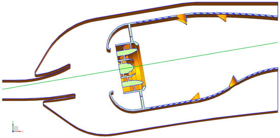
Figure 1.
Single-dome HTR combustor model.
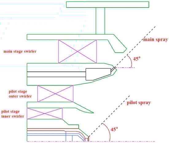
Figure 2.
Structure diagram of the swirler.
This study employs two parameters: the FAR and the equivalence ratio (φ). The FAR serves as a fundamental engineering parameter for defining the overall operating conditions and performance metrics of the combustion chamber. The φ, on the other hand, is used in combustion analysis to characterize the fuel-rich or fuel-lean state of the kerosene-air mixture. Since the φ normalizes the mixture concentration, it enables direct comparison of combustion characteristics under different operating conditions and facilitates correlations with phenomena such as smoke emission. This dual-parameter approach is a standard practice in aero-engine combustion research.
Table 1 presents the single-dome combustor’s key aerodynamic properties and structural characteristics, Table 2 shows the airflow distribution among the components of the combustor, and Table 3 provides the structural parameters of the swirler. Table 3 shows the rotational direction of each stage of the swirlers, observed from the inlet to the outlet. A clockwise rotation is denoted by “+” and a counterclockwise rotation by “−“.

Table 1.
Parameters of the HTR combustor [12].
Table 2.
Air distribution of the combustor [12].
Table 3.
Structural parameters of the swirler [12].
According to Table 1 and Table 2, the dome equivalence ratio is calculated as 0.037 × 14.7/45.05% ≈ 1.21, indicating a fuel-rich dome design. Since the dome equivalence ratio is lower than 1.4, it meets the criterion for suppressing visible smoke in the combustor [1]. Given the distinctive structure of the swirler, assume that all the airflow from the inner swirler and 80% of the airflow from the outer swirler in the pilot stage contribute to forming the traditional swirl cup backflow region. Under idle operating conditions, the FAR is 0.0106. To determine the corresponding equivalence ratio for the swirl cup configuration, the FAR value is multiplied by the stoichiometric air–fuel ratio of aviation kerosene (14.7) and divided by the sum of 0.055 and the product of 0.125 and 0.8. This computation, expressed mathematically as 0.0106 × 14.7/(0.055 + 0.125 × 0.8), results in a derived equivalence ratio of 1.0. When the FAR under blowoff conditions is assumed to be half of the baseline idle condition, the resulting value of 0.005 aligns with the lean flameout limits specified in contemporary military aircraft gas turbine engine standards [26]. Furthermore, assuming that the airflow in the fictitious swirl cup atomizes the fuel, the Air–Liquid Ratio (ALR) for the dome’s swirl cup configuration is derived through the computational formula (0.055 + 0.125 × 0.8)/0.037 ≈ 4.19. This outcome satisfies the required ALR for efficient fuel dispersion within the swirl cup [27,28].
2.2. Wall Configuration Design Law of Flame Tube Convergent Segment
This paper applies the Vitosinski principle, the equal velocity gradient criterion, and the convex-arc contouring approach to design the wall configuration of the convergent segment of the flame tube in the reference model. In the design process, all combustor components, except for the wall configuration of the convergent segment, remain unchanged.
In all three schemes, the center streamline of the convergent segment at the tail of the flame tube follows a double-circular-arc line design. As shown in Figure 3, the design consists of two externally tangent circles with equal radii, and the inflection point (point of tangency) is located at the midpoint of the double-circular-arc line.
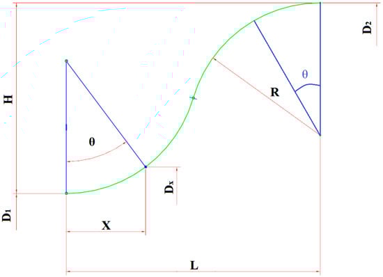
Figure 3.
Double-circular-arc center streamline.
According to Figure 3, the key geometrical parameters of this design are the difference in radii, H, between the inlet and outlet of the convergent segment, and the radius of the arcs, R, defined as follows [24]:
and
Subsequently, the contour of the double-circular-arc line is described by a piecewise function. The equation before the inflection point (X ≤ 0.5 L) is:
where
The equation after the inflection point (X > 0.5 L) is:
where
In Equations (1)–(6), L represents the axial distance of the combustor between the head and tail ends of the double-circular-arc center streamline. D1 and D2 are the diameters at the head and tail ends of the double-circular-arc center streamline, respectively, and X is the axial distance of the combustor measured from the head end of the double-circular-arc center streamline.
The convergence law of the flow-through area at the combustor’s tail typically follows the Vitosinski principle or the equal velocity gradient criterion [24]. The schematic diagram is presented in Figure 4.
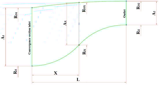
Figure 4.
Flame tube convergent segment wall configuration diagram.
Vitosinski principle (empirical formula):
and
Equal velocity gradient criterion:
In Equations (7)–(9), A1 and A2 are the cross-sectional areas of the inlet and outlet of the convergent segment, respectively. Ro1 and Ro2 are the outer radii of the inlet and outlet cross-sections of the convergent segment, respectively. Ri1 and Ri2 are the inner radii of the inlet and outlet cross-sections of the convergent segment, respectively. L is the axial distance of the combustor between the inlet and outlet cross-sections of the convergent segment, that is, the axial distance of the combustor between the head and tail ends of the double-circular-arc center streamline.
The convex-arc contouring approach [25] proposed in this paper is an optimized design method based on two conventional methods, namely the Vitosinski principle and the equal velocity gradient criterion. The general idea is to first design the wall configuration of the convergent segment of the combustor using the two conventional methods, respectively. Then, based on the simulation results of the two schemes, the lower wall of the convergent segment of the optimal scheme is selected. The upper wall of the convergent segment is replaced by fitting with a long convex-arc line, and a short convex-arc line is used to connect the middle straight-line segment wall of the combustor and the upper wall of the convergent segment.
Figure 5 shows the wall configurations of the combustor’s convergent segment, designed using the Vitosinski principle, the equal velocity gradient criterion, and the convex-arc contouring approach. The corresponding HTR main combustor designs are labeled as Scheme A–C. In Figure 5, the O-axis denotes the central axis of the flame tube, while the P-line indicates the inlet cross-section of the convergent segment.
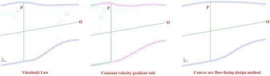
Figure 5.
Different design schemes of flame tube convergent segment.
2.3. Comparative Summary of Design Philosophies
To explicitly delineate the fundamental differences between the three design approaches, a comparative summary is provided in Table 4. This comparison is structured around their underlying principles, defining geometric features, and primary aerodynamic objectives, which serve as the foundational framework for analyzing subsequent results.
Table 4.
Comparison of Design Philosophies and Pathways for the Convergent Segment.
The comparative summary in Table 4 highlights the fundamental differences in design pathways employed by the three schemes. It is important to recognize that Schemes A–C share the common overarching goal of achieving high combustor performance, characterized by low total pressure loss, a uniform outlet flow field, and a high-quality outlet temperature distribution. The critical distinction, however, lies in the underlying principles and strategic approaches taken to reach this goal. Schemes A and B are prescriptive and rule-based; their geometries are derived from empirical and theoretical principles aimed at singular, global flow targets. A direct consequence of these principles is a shared critical geometric feature: a profile with an inflection point. In contrast, Scheme C is phenomenon-driven. Its design prioritizes the elimination of adverse aerodynamic features at their source, resulting in a smooth, inflection-free profile. Therefore, the primary difference is not the ultimate aim but the chosen pathway: Schemes A and B follow predefined rules, which inherently introduce a curvature discontinuity, while Scheme C employs a strategy that actively prevents abrupt flow changes by avoiding the discontinuity itself. This fundamental distinction in design intention and resultant geometry serves as the critical foundation for explaining the subsequent differences in flow structure and combustor performance.
3. Methods
3.1. Numerical Model
3.1.1. RANS Method
ANSYS Fluent software (v2020 R2) was employed in this study for three-dimensional simulations. The governing Navier–Stokes (N-S) equations are as follows:
and
Among them, Equation (10) is the mass conservation equation, Equation (11) is the momentum conservation equation, Equation (12) is the energy conservation equation, and Equation (13) is the state equation of ideal gases.
In multi-species flow systems relevant to combustion, mass conservation is categorized into total mass conservation and species-specific mass conservation. The conservation equation for species i is as follows:
This study adopted the RANS methodology to derive the time-averaged form of the governing N-S equations. The resulting RANS equations are given by:
Compared to the original N-S equations, the time-averaged version incorporates the Reynolds stress term , which represents the effects of turbulence. To connect the Reynolds stress with the velocity gradient, Boussinesq’s hypothesis is commonly applied, thereby converting the Reynolds stress solution into the determination of turbulent viscosity µt. The specific expression of the Boussinesq’s hypothesis is given by [29]:
3.1.2. Turbulent Flow Model and Radiation Model
This research employed the RKE two-equation turbulence model. Grounded in Boussinesq’s hypothesis, the model is particularly suited for scenarios involving intense swirling flow. In the RKE model, the transport equations for variables k and ε are presented as follows:
and
In this paper, the Discrete Ordinates (DO) model was selected for radiation calculation. The Radiation Transfer Equation (RTE) is as follows:
3.1.3. Discrete Phase Model and Combustion Model
Aviation kerosene (molecular formula C12H23) was selected as the fuel for the HTR main combustor. The Discrete Phase Model (DPM) uses the Euler–Lagrange method to simulate the interaction between dispersed liquid droplets and a gaseous continuum. This model relies on two crucial premises: (1) dispersed-phase particles exhibit substantially greater mass density compared to the surrounding medium, and (2) interparticle forces are considered negligible.
A non-premixed combustion model based on the mixture fraction approach and the equilibrium chemistry assumption was employed. The thermochemical state at any location during combustion (including species mass fraction Yi, density ρ, and temperature T) can be related to the local mixture fraction f. The combustion process is simplified to a mixing problem involving the fuel, oxidizer, and intermediate product species. The reaction system includes 11 species: H2, OH, O2, H2O(l), H2O(g), C(s), N2, CO, CO2, CH4, and C12H23.
For combustion reactions considering only the C, H, and O elements present in aviation kerosene, the mixture fraction can be represented as follows:
3.2. Grids Division and Boundary Conditions
3.2.1. Partition Processing and Grids Division
In this paper, the region corresponding to one dome of the full annular main combustor is selected, and the ANSYS pre-processing software NX (v12.0) and ICEM CFD (v2020 R2) are used for structural modeling and meshing. The computational domain of this single-dome combustor encompasses the pre-diffuser, inner and outer bifurcated channels, a swirler, and a flame tube, among other components, to enable coupled calculations of the entire flow domain within the combustor. The flame tube’s cooling holes are designed as dense multi-inclined holes, making structured meshing too time- and labor-intensive. Therefore, unstructured meshing is used in this study. Considering the large number of meshes, the complex structure of the combustor, and the performance of the working computer, during meshing, the overall structure of the combustor is partitioned, which is convenient for searching, error correction, and effectively controlling the mesh density. Taking the reference model as an example, as shown in Figure 6 and Figure 7.
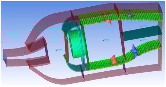
Figure 6.
Partitioning of the HTR combustor.
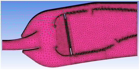
Figure 7.
Meshing of the HTR combustor.
This study employed the Grid Convergence Index (GCI) [30] for grid independence verification. Specifically, Table 5 presents the GCI values for the Total Pressure Loss Coefficient (TPLC) across the combustor. As shown in Table 5, the grid count of the N2 scheme is 61.2% less than that of the N1 scheme, resulting in a significant reduction in computational cost, while its GCIfine value is 0.6244%, meeting the required standard.
Table 5.
GCI values for TPLC across the combustor [31].
Three schemes with different grid densities listed in Table 5 were utilized. Figure 8 compares the radial distribution of the axial velocity at the center of the recirculation zone under cold-flow conditions for these three schemes. It can be observed from Figure 8 that the reflux intensity at the center of the recirculation zone increases with grid refinement. The circumferentially averaged axial velocity at this location is −3.8 [m/s] for the finest grid (N1), −3.4 [m/s] for N2, and −1.1 [m/s] for N3. Therefore, considering both computational cost and accuracy requirements, the N2 scheme is deemed more feasible. In other words, the grid is considered independent when the velocity distribution no longer changes significantly with further grid refinement. Consequently, the final total grid count was determined to be 11.89 million.
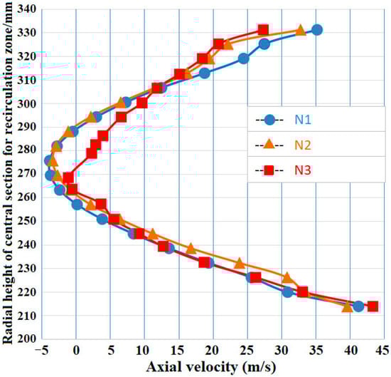
Figure 8.
Comparison of the axial velocity distributions among the three sets of schemes [31].
3.2.2. Boundary Conditions and Solution Methods
Within the numerical model, airflow is assumed to behave as an incompressible medium. The inlet cross-section of the combustion chamber is defined as the mass-flow-inlet boundary condition, whereas the outlet cross-section of the combustor liner is defined as the outflow boundary condition. For the single-dome combustion chamber, the two sides of the whole fluid domain adopt rotational periodic boundary conditions. The reference pressure point is situated at the center of the combustor inlet. The diffuser and casing walls, similar to the two turbine cooling bleed outlets, are defined as adiabatic no-slip walls. The remaining walls are classified as radiative walls. The flow distribution to the dome assembly, which includes swirlers at all stages and cooling holes, along with liner perforations (e.g., primary/dilution hole jets and multi-inclined cooling passages), is determined through iterative fluid dynamics coupling simulations.
The numerical solver employs the SIMPLE algorithm (Semi-Implicit Method for Pressure-Linked Equations) to resolve pressure–velocity coupling dynamics. For spatial discretization of conservation equations, the Green–Gauss Cell-Based approach is selected for computing gradients, while pressure interpolation utilizes the Standard scheme. Furthermore, the second-order upwind difference scheme is applied to the remaining governing equations (such as Momentum, Energy, etc.).
Numerical convergence during simulation is evaluated through the iterative evolution of solution metrics and critical flow variables. The tracked parameters include: (1) mean flow velocity in the recirculation core region, (2) total temperatures (mean and peak values) at the combustor outlet, and (3) total pressure averages. The convergence criterion is that each residual must be less than 0.001, and the variation in monitored data over 100 iterations should not exceed 1%.
3.3. Comparative Evaluation
A steady-state simulation of the full-process, three-dimensional, turbulent, two-phase reactive flow with recirculation in a single annular HTR main combustor [32] was performed using the same mathematical and physical model employed in this paper. The simulation results were compared with corresponding performance test data. This comparative exercise is conducted with a dual purpose. Its primary role is not only to validate the reliability of the numerical methodology itself by benchmarking against a known case [32], but also, and more importantly, to provide a credible foundation for the subsequent comparative analysis. This validated foundation enables a fair performance comparison of the three proposed convergent segment designs (Schemes A–C), ensuring that observed differences are attributable to the geometric configurations rather than numerical inaccuracies.
3.3.1. Total Pressure Recovery Coefficient
Figure 9 illustrates a comparative analysis of computational modeling outcomes and empirical measurements concerning the influence of the inlet flow capacity, represented by the mass flow function q(λ), on the total pressure recovery coefficient under cold-flow conditions. The variation trends of both are consistent. The Total Pressure Recovery Coefficient (TPRC), defined as the ratio of the average total pressure at the combustor outlet section (Pt4) to that at the inlet section (Pt3) (i.e., TPRC = Pt4/Pt3), decreases as q(λ) increases. Under design conditions, numerical predictions yield a total pressure recovery coefficient that deviates by approximately 1.4% from experimentally observed values.
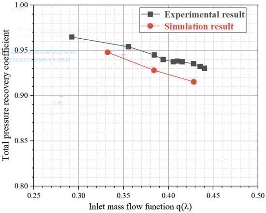
Figure 9.
Influence of q(λ) on the TPRC [2,32].
The experimental and simulation data points in Figure 9 are cited directly from Reference [32]. Although not all operational points are covered, the three key points (low, medium, and high load) adequately capture the core physical trends.
3.3.2. Combustion Efficiency
The combustion efficiency ηc of the full annular combustor is measured by the gas-analysis method. The influence of the universal combustion efficiency criterion θc on ηc is presented, as shown in Figure 10. The formula for the definition of the θc is:
as defined in reference [32].
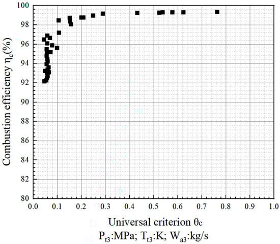
Figure 10.
Influence of the θc on ηc [2,32].
The parameter θc integrates three key inlet parameters of the full annular combustor (with 20 heads)—namely, the inlet pressure Pt3, temperature Tt3, and air mass flow rate Wa3—into a comprehensive evaluation metric. It is used to comprehensively assess the inlet conditions of the full annular combustor and reflect the coupled effects of inlet pressure, temperature, and air mass flow rate on the combustion process.
As shown in Figure 10, ηc increases as θc increases. When the θc exceeds 0.8, ηc approaches 100%. Under design conditions, the θc of this combustor is 2.388. As illustrated in Figure 10, ηc is approximately 100%, whereas the simulation results yield a result of 99.80%. This demonstrates that the numerical calculation of combustion efficiency aligns well with the component test results. For states with high inlet variables (e.g., temperature and pressure), the combustion efficiency derived from the non-premixed PDF combustion framework is reliable.
3.3.3. Overall Temperature Distribution Factor
Figure 11 illustrates the temperature distribution patterns at the outlet derived from experimental component analysis. Specifically, SOTDF represents the combustor’s performance severity index [32]. Overall Temperature Distribution Factor (OTDF) quantifies the uniformity of temperature distribution at the outlet. This parameter is mathematically expressed as the quotient of the maximum-to-average temperature differential relative to the combustor’s total temperature rise. Furthermore, the OTDF value depicted in Figure 11 corresponds to the mean measurement across the single-dome sector region. The mathematical expressions defining SOTDF and OTDF are presented below:
as defined in reference [32], and
where T4ave represents the average temperature at the flame tube outlet, T4max represents the maximum temperature at the flame tube outlet, and △T4−3 represents the combustor’s temperature rise (T4ave − T3ave). W3c represents the available air volume of the full annular main combustor. Since turbine cooling airflow is not involved in combustion reactions, the usable airflow is the combustor’s inlet air minus the turbine cooling air volume.
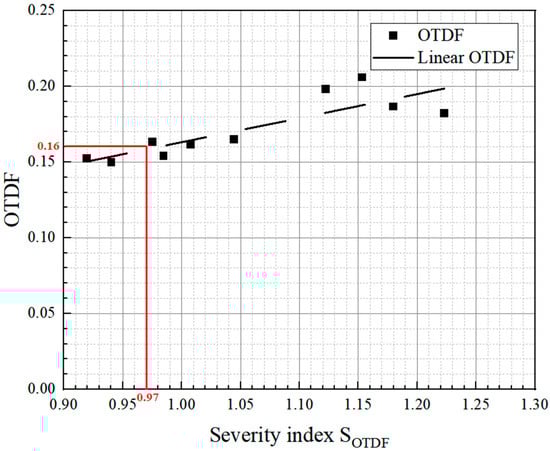
Figure 11.
Influence of the SOTDF on OTDF [2,32].
At the combustor’s design point, SOTDF = 0.97. As shown in Figure 11, the experimental OTDF value is 0.16, while the simulation-based calculated value is 0.168. This shows that the calculated value of OTDF closely matches the experimental value.
3.3.4. Radial Temperature Distribution Factor
Illustrated in Figure 12 is a comparison between computational models and experimental assessments regarding the mean Radial Temperature Distribution Factor (RTDF) profiles. This parameter quantifies the proportionate variance between T4avc,i, representing the circumferentially averaged radial temperature at the combustor outlet, and T4ave, the mean temperature at the outlet, relative to the temperature difference between the inlet and outlet (T4ave − T3ave). The reported RTDF corresponds to the peak magnitude identified across the radial extent of the distribution profile.
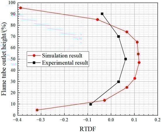
Figure 12.
Comparison of the RTDF curves [2,32].
As shown in Figure 12, both the simulated and experimental values of RTDF reach their maximum at the relative outlet height of r/R = 50%. When r/R is less than 50%, the simulated and experimental RTDF values increase with rising r/R, but the rate of increase gradually slows down. When r/R exceeds 50%, both the simulated and experimental RTDF values decrease as r/R increases, and the rate of decrease accelerates. For quantitative analysis of their variation trends, the Pearson Correlation Coefficient (rp) [33] was employed. Using the radial heights of the experimental data points as a reference, the corresponding simulated values at these radial heights were determined via linear interpolation. The calculation results are presented in Table 6.
where Xi and Yi represent the experimental and simulated data pairs, respectively, corresponding to the i-th identical radial position r/R.
Table 6.
Calculated RTDF at different radial positions and parameter rp [31].
As shown in Table 6, the rp is 0.89, indicating a very strong positive correlation between the simulated and experimental RTDF curves. This means the variation trends of the simulated and experimental RTDF values are highly consistent. However, in the regions near the inner and outer annular walls of the flame tube, the simulated values are generally lower than the experimental values. This deviation primarily stems from the inherent limitations of the RANS turbulence model used in our simulation. This type of time-averaged model has deficiencies in predicting the complex mixing process between the cooling film and the main airflow near the walls, tending to overestimate the mixing degree, which leads to an underestimation of the local temperature (and thus the RTDF value) in these regions. In the overall central region of the flame tube outlet (spanning approximately 10% to 80% of the radial height), the simulated RTDF values and their peak are systematically higher than the experimentally measured values. This discrepancy arises mainly because the experimental hardware must include solid sidewalls for structural integrity. These sidewalls act as a heat sink, causing the temperature measured by the thermocouples to be systematically lower due to heat loss via radiation and conduction to the cooler sidewalls. In contrast, the numerical model employs periodic boundary conditions, eliminating such physical sidewalls and their associated heat sink effect. Consequently, the simulation calculates the adiabatic fluid temperature, unaffected by this experimental heat loss. This specific deviation thus precisely reveals a physical limitation of the experimental measurement technique, rather than indicating a fundamental flaw in the numerical model.
In conclusion, the adopted mathematical–physical framework calculates the combustor’s TPRC with a minor underprediction relative to experimental measurements, accurately predicts combustion efficiency and OTDF, and yields elevated RTDF predictions while preserving trend congruence. A comparative analysis of empirical and computational outcomes confirms the general validity of the numerical methodology. The selected model can effectively predict combustor performance and assist in screening design options.
3.4. Outlet Section Data Extraction Methodology
To facilitate the quantitative analysis of the flow field uniformity at the flame tube outlet, this paper introduces the concept of standard deviation to characterize the uniformity of the total pressure distribution over the outlet cross-section. The Outlet Total Pressure Distribution Factor (OPDF) is defined as the ratio of the standard deviation S to the mean total pressure at the outlet P4ave, as follows:
and
To further investigate the total pressure distribution at different radial heights of the outlet, this study defines the Average Radial Total Pressure Distribution Factor (RPDF) curve based on the RTDF curve. Specifically, the RPDF is defined as the ratio of two pressure differentials: the absolute difference between the circumferential average of radial total pressures at the combustor exit and the mean exit pressure, divided by the difference between the mean total pressures at the combustor’s entrance and exit, as follows:
The RPDF value is the maximum value calculated along the radial height of the RPDF curve.
In this study, the flame tube outlet is divided into 20 total pressure distribution zones along the radial direction, where N = 20. In Equations (26)–(28), P4avc,i represents the circumferentially averaged total pressure of the th total pressure distribution zone at the outlet. P4ave represents the mass-weighted average total pressure at the outlet, while P3ave represents the mass-weighted average total pressure at the combustor inlet. Smaller values of OPDF and RPDF indicate a more uniform pressure distribution.
To quantitatively analyze the radial distribution uniformity of the total pressure and total temperature at the flame tube outlet, a unified data extraction method based on equidistant division along the radial height was employed. The core of this methodology is that the total pressure distribution zones and the total temperature distribution zones share identical geometric division criteria, ensuring strict comparability of different performance parameters at identical spatial locations. The specific procedure is detailed below.
- 1.
- Division Basis and Geometric Definition
The radial height H of the flame tube outlet cross-section (an annular plane perpendicular to the central axis of the full annular combustor), defined as the vertical distance from the inner annular wall to the outer annular wall at the outlet, serves as the basis for division. This radial height H is divided into 20 intervals of equal spacing. The height of each interval is Δh = H/20. These division points define 20 infinitely thin annular bands perpendicular to the central axis of the full annular combustor. Each annular band constitutes a basic data analysis unit, referred to as a “distribution zone”.
- 2.
- Data Extraction and Processing ProcedureFor each distribution zone (the i-th zone), the following procedure is executed:
- (1)
- Data Acquisition: Extract the total pressure values (for OPDF and RPDF analysis) or the total temperature values (for RTDF analysis) at all grid nodes within the corresponding annulus.
- (2)
- Circumferential averaging: Calculate the circumferentially averaged value of the acquired data to obtain a representative total pressure value P4avc,i or total temperature value T4avc,i for that specific radial location.
- (3)
- Result Application: The set of these 20 circumferentially averaged values at different radial locations is precisely the data used to calculate the OPDF/RPDF/RTDF values and to plot the RPDF/RTDF curves. The abscissa (X-axis) of the RPDF/RTDF curves is the RPDF/RTDF value of the distribution zone, and the ordinate (Y-axis) is the corresponding radial height normalized by the total radial height H (expressed as a percentage).
- 3.
- Rationale for the Number of Zones (N = 20)
The selection of 20 distribution zones (N = 20) is an optimized outcome resulting from a trade-off between data resolution and statistical stability. An excessively large number of zones (large N) reduces the data sample size per zone, increasing statistical uncertainty. Conversely, too few zones (small N) over-smooth the data, failing to capture detailed gradients in the radial distribution. Based on pre-mesh-sensitivity trial calculations, it was determined that N = 20 can effectively resolve the key features of the RPDF and RTDF curves (such as peak location and distribution trend) under the grid density used in this study, while simultaneously ensuring a sufficient number of grid points within each zone for reliable circumferential averaging.
In summary, the standardized data extraction procedure described in this section provides a unified and reliable foundation for the objective comparison of outlet performance among different schemes (Scheme A–C) in Section 4.
4. Results and Discussion
4.1. Comparison of Two Conventional Design Law Schemes
4.1.1. Comparison of Flow Field Distributions for Scheme A and Scheme B
Under the design conditions, Figure 13 shows the velocity distribution nephograms of Scheme A (designed using the Vitosinski principle) and Scheme B (designed using the equal velocity gradient criterion) on the combustor’s central cross-section. Figure 14 compares the upper and lower wall configurations of the convergent segments of both schemes in the same coordinate system. Figure 14 shows inflection points at points M and N on the upper and lower wall configuration curves of the convergent segments of both Schemes A and B.
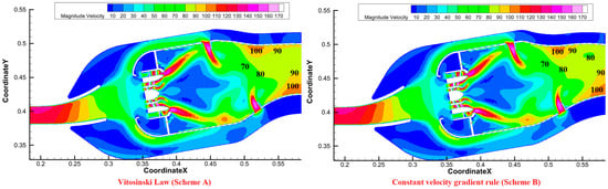
Figure 13.
Comparison of the velocity distribution cloud images of Scheme A and Scheme B on the central section.
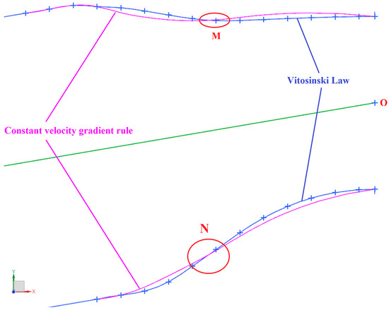
Figure 14.
Comparison of the upper wall configuration of the convergent segment of Scheme A and Scheme B.
The analysis of the velocity contours (Figure 13) first confirms a fundamental similarity between Schemes A and B: both feature an upper wall profile with an inflection point, as defined in Table 4. This shared geometric characteristic is the root cause of the localized high-velocity region observed near point M in the upper half of the convergent segment for both schemes. The rapid flow turning at the inflection point accelerates the flow, creating a semi-circular high-velocity zone. However, a critical difference emerges in the flow evolution along the segment. In Scheme A, the velocity increases more gradually before point M and decreases more slowly after it, resulting in a smoother overall acceleration. This can be attributed to the specific wall contour dictated by the Vitosinski principle, which provides a more gradual area convergence around the inflection point compared to the sharper contraction enforced by the equal velocity gradient criterion in Scheme B. This subtle geometric distinction, though both schemes possess an inflection point, leads to a discernible difference in flow development, which subsequently influences outlet uniformity.
This comparative analysis reveals that although the specific implementation of the wall contour (Vitosinski vs. equal velocity gradient) leads to discernible differences in flow development, both Schemes A and B suffer from a common root cause of flow imperfection: the inflection point on the upper wall (Figure 14). This geometric discontinuity is a key defect that triggers non-uniformity by forcing abrupt flow turning and local acceleration. This fundamental understanding frames our investigation of Scheme C, which probes whether eliminating the inflection point itself, via a smooth convex-arc contour, can provide a definitive solution.
Table 7 presents the calculated values of the total pressure distribution uniformity indices at the outlet for both Schemes A and B. Figure 15 presents a comparison of the RTDF curves at the outlet for both schemes.
Table 7.
Total pressure distribution uniformity index of flame tube outlet for Scheme A and Scheme B.
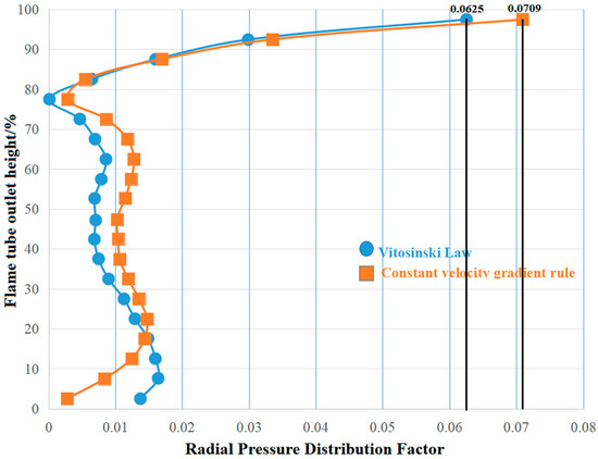
Figure 15.
Comparison of RPDF curves between Scheme A and Scheme B.
As shown in Table 7, the OPDF of Scheme B is 1.10 times that of Scheme A, and the RPDF of Scheme B is 1.13 times that of Scheme A. Therefore, compared to Scheme B, Scheme A exhibits better uniformity in the total pressure distribution at the flame tube outlet. As shown in Figure 15, above 20% of the radial height at the outlet, the RPDF value of Scheme A is basically lower than that of Scheme B. Below 20% of the radial height at the outlet cross-section, the RPDF value of Scheme A is higher than that of Scheme B. In other words, the uniformity of the total pressure distribution at the outlet of Scheme A is generally better than that of Scheme B across the radial height of the outlet. Only in the region where the radial height is below 20% does Scheme B exhibit better uniformity in total pressure distribution than Scheme A. However, the difference in RPDF values between the two schemes in the region where the radial height is below 20% is not significant, with the maximum difference not exceeding 0.8%.
4.1.2. Comparison of Temperature Distributions for Scheme A and Scheme B
Under the design conditions, the temperature distribution nephograms of Scheme A, designed using the Vitosinski principle, and Scheme B, designed using the equal velocity gradient criterion on the combustor’s central cross-section, are shown in Figure 16. The numbers in the figure denote isotherms, and their values represent 1/100 of the actual temperature value [K]. For example, the annotation “25” corresponds to 2500 [K].
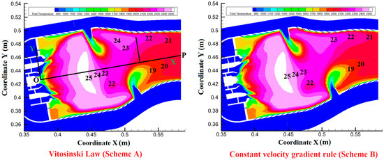
Figure 16.
Comparison of the temperature distribution cloud images of scheme A and scheme B on the central section.
As shown in Figure 16, the temperature distributions in the primary zone for Scheme A and Scheme B are nearly identical, while slight differences are observed in the dilution zone. These differences are attributed to the distinct wall configurations of the convergent segment of the flame tubes, whereas the other components of the combustion chamber remain unchanged.
In Figure 16, point O represents the center of the exit of the pilot stage fuel nozzle, and point P represents the center of the flame tube outlet. To further investigate the temperature distribution differences in the dilution zone, a rectangular coordinate system is established with point O as the origin, and the line connecting points O and P is designated as the X-axis. The rightmost points of the 2100 [K], 2200 [K], and 2300 [K] temperature contours in the dilution zone are projected onto the X-axis, and the corresponding X-values are recorded. These values, presented in Table 8 (units: [mm]), show that the gas temperature in the dilution zone of Scheme A is more rapidly adjusted by the dilution air flow.
Table 8.
Projection coordinates of the critical point on the right side of the temperature contour for Scheme A and Scheme B.
4.1.3. Comparison of Various Outlet Performance Indicators for Scheme A and Scheme B
Conventionally, combustor’s TPL is characterized by the disparity between inlet and outlet total pressure magnitudes. This thermodynamic parameter, when normalized against the inlet total pressure, defines the TPLC, which is mathematically formulated as:
where Pt3 represents the total pressure at the combustor’s inlet, while Pt4 represents the total pressure at the flame tube’s outlet.
This study investigates the TPL in the flame tubes of Schemes A and B, from the dilution segment’s inlet to the tail outlet. The TPLC of the flame tube’s convergent segment is defined as the ratio of the total pressure difference between the inlet of the convergent segment and the outlet of the flame tube to the total pressure at the combustor’s inlet. The formula is as follows:
where Pci represents the total pressure at the inlet of the flame tube’s convergent segment. To avoid interference from the primary holes, the chosen inlet is cross-section N, which is perpendicular to the flame tube’s central axis, rather than the vertical cross-section P, as illustrated in Figure 17.
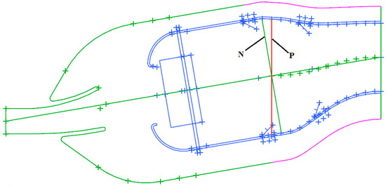
Figure 17.
Selection of inlet section of flame tube convergent segment.
Table 9 presents the calculated combustor outlet performance for Scheme A and Scheme B. Figure 18 compares the RTDF curves of both schemes at the flame tube’s outlet cross-section, and Figure 19 provides a comparison of the temperature distribution at the same cross-section. As shown in Table 9, the TPLC of Scheme A is slightly higher than that of Scheme B. However, the TPLCs for both schemes are below 6%, which meets the HTR combustor’s performance requirement range of 5–6%. The slightly higher TPLC in Scheme A compared to Scheme B is due to a marginally greater pressure loss in the convergent segment of Scheme A. Nevertheless, the TPLCs of the convergent segments for both schemes are below 0.4%, which satisfies the design specifications. Furthermore, the OTDF values for both schemes are below 0.2, and the RTDF values fall within the range of 0.08–0.12. This indicates that both the OTDF and RTDF values comply with the performance requirements of HTR main combustors with a temperature rise of approximately 1150 [K].
Table 9.
Calculation results for Scheme A and Scheme B.
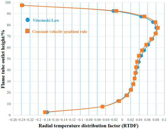
Figure 18.
Comparison of RTDF curves between Scheme A and Scheme B.
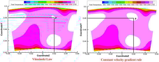
Figure 19.
Comparison of temperature distribution nephogram of flame tube outlet between Scheme A and Scheme B.
The performance comparison (Table 9) reveals that Scheme A achieves superior outlet temperature distribution quality and combustion efficiency compared to Scheme B. This trend is fundamentally rooted in the differences in their convergent segment wall contours. Although both schemes incorporate an inflection point, the Vitosinski principle employed in Scheme A results in a more gradual area convergence around this point. This geometric subtlety fosters a more controlled flow acceleration. The resulting flow field uniformity, established throughout the convergent segment, directly enables more effective penetration and mixing of the dilution jets, which is ultimately reflected in the superior temperature distribution at the flame tube outlet.
The detailed outlet temperature profiles, illustrated in Figure 18 and Figure 19, provide clear evidence for these superior distribution qualities. Firstly, the reduction in the RTDF value for Scheme A is directly evidenced by its RTDF curve in Figure 18, which exhibits gentler fluctuations with a lower peak value. This quantitative relationship is corroborated by the temperature nephogram in Figure 19, which shows a significantly smaller high-temperature region (>2100 [K]) near point P in Scheme A compared to Scheme B. Secondly, the superior OTDF value of Scheme A stems from the fact that it achieves a higher mass-weighted average temperature at the outlet concurrently with a lower maximum outlet temperature than Scheme B.
This apparent paradox—where a slightly higher pressure loss in a component correlates with superior overall performance—is resolved by analyzing the causal chain from geometry to the flow field and finally to combustion outcomes. Although both Schemes A and B incorporate an inflection point that inherently induces a localized loss, the more controlled flow acceleration in Scheme A’s convergent segment (as analyzed in Section 4.1.1), resulting from its specific Vitosinski contour, yields a more uniform flow field at the dilution zone inlet. This enhanced flow uniformity promotes deeper penetration and more effective mixing of the transverse air jets from the dilution holes.
The direct result of this superior flow organization is a more rapid and effective adjustment of the temperature field within the dilution zone itself, as quantitatively demonstrated by the faster downstream retreat of high-temperature contours (e.g., 2300 [K], 2200 [K]) in Scheme A compared to Scheme B (refer to Table 8 in Section 4.1.2). It is precisely this more efficient thermal adjustment process in the dilution zone that is the fundamental reason why Scheme A achieves a higher-quality temperature distribution (i.e., lower OTDF and RTDF values) at the combustor outlet.
Therefore, the net performance gain of Scheme A lies in its superior flow management strategy: the marginally higher TPL in its convergent segment is a beneficial investment that pays off as a significant improvement in combustion completeness and outlet temperature distribution quality. This demonstrates that even between two designs sharing the same key curvature discontinuity (the inflection point), the precise implementation of the wall contour—dictated by the Vitosinski principle versus the equal velocity gradient criterion—has a profound impact on the final outcome.
In summary, considering the flow field distribution, temperature distribution, and outlet performance of the combustors in both schemes, the HTR combustor in Scheme A, which applies the Vitosinski principle, demonstrates superior performance.
4.2. Comparison of the Optimal Conventional and Convex-Arc Flow-Facing Schemes
To investigate the impact of the wall configuration in the flame tube convergent segment on the performance of the HTR main combustor, a comparative analysis is conducted between the combustor in Scheme B, which is based on the Vitosinski principle selected from two conventional design laws, and the combustor in Scheme C, which uses the convex-arc contouring approach.
4.2.1. Comparison of Flow Field Distributions for Scheme A and Scheme C
Under the design conditions, the velocity distribution maps for Scheme A, designed using the Vitosinski principle, and Scheme C, designed using the convex-arc contouring approach, on the combustor’s central cross-section are shown in Figure 20. Figure 21 compares the upper and lower wall configurations of the convergent segments of the two schemes in the same coordinate system. Figure 21 illustrates that the upper wall configuration curve of the convergent segment of the flame tube in Scheme A has an inflection point, while Scheme C’s does not.
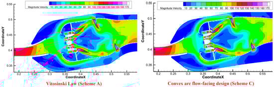
Figure 20.
Comparison of the velocity distribution cloud images of Scheme A and Scheme C on the central section.
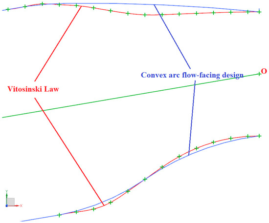
Figure 21.
Comparison of the upper wall configuration of the convergent segment of Scheme A and Scheme C.
The velocity distributions in Figure 20 reveal a fundamental aerodynamic distinction in the upper section of the dilution zone, directly attributable to the core geometric difference summarized in Table 4: the presence or absence of an inflection point on the upper wall. Scheme A, with its inflection-point profile, exhibits a distinct, concentrated high-velocity region anchored precisely at the inflection point. This is a direct manifestation of the localized flow acceleration induced by the abrupt flow turning at this point of sharp curvature change. In stark contrast, the velocity field in Scheme C, which features a smooth, inflection-free profile, demonstrates remarkably uniform and gradual acceleration, completely free of such adverse flow structures. The elimination of the inflection point in Scheme C’s design successfully prevents the abrupt flow turning that generates the high-speed zone in Scheme A.
Furthermore, a critical difference is observed in the lower section near the flame tube outlet. The high-velocity regions (e.g., 90–100 [m/s] and 100–110 [m/s]) in Scheme C are notably smaller than those in Scheme A. As illustrated in Figure 21, this is a result of the convex-arc flow-facing design of the lower wall in Scheme C, which provides a gentler slope compared to the contour of Scheme A. This gentler slope results in a larger cross-sectional area and combustion flow space near the outlet for Scheme C, leading to a reduction in flow velocity.
This visual evidence from both the upper and lower sections of the convergent segment powerfully confirms that: (1) the inflection point on the upper wall acts as a generator of flow non-uniformity, and its elimination is key to achieving superior flow uniformity, and (2) the gentler slope of the lower wall contour in Scheme C contributes to a more favorable pressure recovery and reduced acceleration near the outlet. The combined effect of these geometric optimizations in Scheme C leads to an overall superior flow field.
Table 10 shows the calculated values of the total pressure distribution uniformity indices at the flame tube outlet for both Scheme A and Scheme C. Figure 22 compares the RTDF curves at the outlet for both schemes.
Table 10.
Total pressure distribution uniformity index of flame tube outlet for Scheme A and Scheme C.
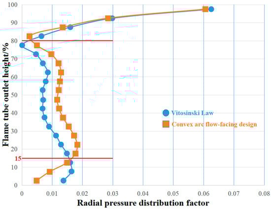
Figure 22.
Comparison of RPDF curves between Scheme A and Scheme C.
As shown in Table 10, the OPDF of Scheme C is 1.04 times that of Scheme A. Therefore, the overall total pressure distribution uniformity at the flame tube outlet is better in Scheme A. Regarding the RPDF, the value for Scheme A is 1.03 times that of Scheme C. However, as shown in the RPDF curve in Figure 22, within the range of 15–80% radial height of the outlet cross-section, the RPDF value of Scheme A is lower than that of Scheme C. Outside this range (less than 15% and greater than 80%), the RPDF value of Scheme A is higher than that of Scheme C. In summary, the overall total pressure distribution uniformity at the outlet is better in Scheme A than in Scheme C. However, in regions where the radial height is less than 15% or greater than 80%, Scheme C exhibits better uniformity than Scheme A.
4.2.2. Comparison of Temperature Distributions for Scheme A and Scheme C
Figure 23 provides a comparative visualization of the temperature distribution nephograms on the combustor’s central cross-section under the design condition, contrasting Scheme A (incorporating the Vitosinski principle) with Scheme C (utilizing the convex-arc contouring approach). The annotation convention for the temperature isovalues follows the same rule as specified in Figure 16.
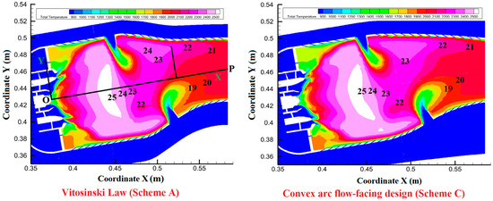
Figure 23.
Comparison of the temperature distribution cloud images of scheme A and scheme C on the central section.
As shown in Figure 23, the temperature distributions in the primary zone for Scheme A and Scheme C are nearly identical, with minor differences observed in the dilution zone. This is due to the differing wall configurations of the convergent segments of the flame tubes, while the other combustor components remain unchanged.
To further analyze the temperature distribution differences within the dilution zone, the rightmost points of the 2100 [K], 2200 [K], and 2300 [K] temperature contours in Figure 23 are projected onto the X-axis (OP line), and the corresponding X-values are measured, as shown in Table 11 (unit: [mm]). As shown in Table 11, the rates at which the gas temperatures in the dilution zones of Scheme A and Scheme C are adjusted by the dilution air flow do not differ significantly.
Table 11.
Projection coordinates of the critical point on the right side of the temperature contour for Scheme A and Scheme C.
4.2.3. Comparison of Various Outlet Performance Indicators for Scheme A and Scheme C
The calculated combustor outlet performance for Scheme A and Scheme C is presented in Table 12. Figure 24 and Figure 25 show the comparison of RTDF curves and temperature distribution nephograms at the flame tube outlet for both schemes.
Table 12.
Calculation results for Scheme A and Scheme C.
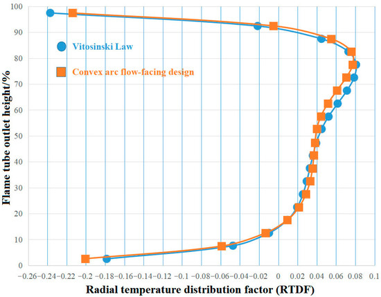
Figure 24.
Comparison of RTDF curves between Scheme A and Scheme C.
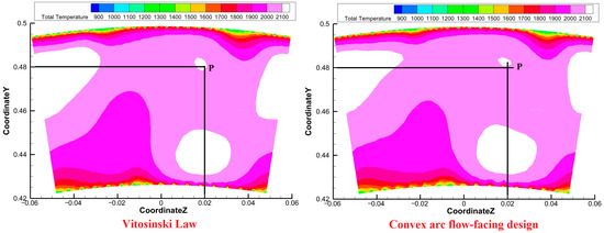
Figure 25.
Comparison of temperature distribution nephogram of flame tube outlet between Scheme A and Scheme C.
The comprehensive performance comparison (Table 12) unequivocally demonstrates that Scheme C achieves the best overall performance, fundamentally attributable to its inflection-free convex-arc design philosophy. This design proactively eliminates the geometric feature (the inflection point) that is a known precursor to flow separation and adverse pressure gradients. By doing so, it fosters a highly uniform flow field that optimizes dilution mixing and combustion efficiency. The quantitative data shows that Scheme C achieves a comparable overall TPLC to Scheme A but with a significantly lower TPLC in the convergent segment (εcs). This reduction in component loss is a direct result of eliminating the adverse flow losses inherently associated with the inflection point in Scheme A. Furthermore, Scheme C exhibits higher combustion efficiency and superior outlet temperature distribution quality, evidenced by its lower OTDF and RTDF. Specifically, Scheme C achieves a higher average outlet temperature alongside a lower maximum outlet temperature, resulting in a smaller OTDF value. Although the OTDF values of both schemes are below 0.2, satisfying the performance requirements, Scheme C’s is lower. The RTDF curves (Figure 24) of both schemes show a single peak in the upper half of the outlet; however, the curve for Scheme C fluctuates more gradually with a lower peak value, consistent with its lower RTDF value compared to Scheme A, as quantitatively listed in Table 12, with both values residing within the acceptable performance band (0.08–0.12). This is visually corroborated by the temperature nephograms (Figure 25), where the high-temperature regions (>2100 [K]) in the upper half of the outlet are smaller in Scheme C compared to Scheme A.
The synergy of these results—reduced component pressure loss alongside enhanced combustion efficiency and outlet temperature distribution—stems from the fundamental advantages of the inflection-free design. The superior performance is attributed to the improved flow uniformity enabled by the smooth, inflection-free contour of Scheme C, as analyzed in Section 4.2.1 and Section 4.2.2. This improved uniformity promotes more effective mixing in the dilution zone. The larger volume of the convergent segment in Scheme C (as shown in Figure 21) further allows for more complete combustion. This synergy effectively demonstrates the fundamental advantage of the inflection-free design paradigm: by prioritizing flow uniformity over prescribed rules, Scheme C successfully avoids the aerodynamic penalties introduced by the geometric discontinuity of an inflection point.
It is worth noting that a more comprehensive analysis, detailed in Section 4.2.1, reveals further nuances. While Scheme C’s RPDF is the best among the three schemes, its OPDF ranks in the middle. This suggests that the primary advantage of the inflection-free design lies in its superior management of the flow field in the radial direction, which is critically linked to the RTDF. Additionally, the rate of temperature adjustment in the dilution zone for Scheme C is intermediate between the other two schemes, indicating that the emphasis of the convex-arc design is on achieving optimal flow uniformity and combustion completeness rather than maximizing a single intermediate parameter. These detailed observations further enrich the understanding of the mechanisms behind Scheme C’s overall performance superiority and validate that the phenomenon-driven, inflection-free design paradigm (Scheme C) provides a more optimal solution than conventional prescriptive approaches (Scheme A).
5. Conclusions
This study systematically investigates the influence of the flame tube convergent segment wall configuration on the performance of an HTR triple-swirler annular main combustor. Three configurations were designed and evaluated: the Vitosinski principle (Scheme A)—an empirical approach for flow area convergence based on historical data; the equal velocity gradient criterion (Scheme B)—a method aiming to maintain a constant velocity gradient along the segment; and the convex-arc contouring approach (Scheme C)—a novel technique proposed in this study to optimize wall shapes using convex arcs for enhanced flow dynamics. Three-dimensional numerical simulations of flow and combustion were conducted for these schemes under takeoff conditions, and their performance was compared. The results demonstrate that Scheme C achieved the best overall performance, with superior flow uniformity and combustion efficiency.
This comparative study reveals the intrinsic causal chain linking ‘geometric feature—flow field structure—combustion performance’:
- (1)
- Geometric Root Cause: The inflection point on the upper wall contour is a key geometric defect that induces local flow acceleration and separation, compromising flow uniformity.
- (2)
- Flow Field Effect: The presence of an inflection point leads to localized high-velocity regions in the convergent segment, whereas a smooth convex-arc profile produces uniform and gradual flow acceleration.
- (3)
- Performance Outcome: The uniformity of the flow field directly determines the efficiency of mixing. By employing an inflection-free design, Scheme C achieves the most uniform flow field, which translates into the best outlet temperature distribution factors (OTDF, RTDF) and the highest combustion efficiency, while maintaining the lowest pressure loss due to its hydraulically smooth flow path.
The comprehensive analysis yields three principal findings that advance the design methodology for high FAR combustion systems:
- (1)
- The Inflection Point as a Fundamental Geometric Defect. The comparative analysis confirms that the inflection point—a geometric feature inherent to the conventional design principles governing Schemes A and B (as defined in Table 4)—acts as a critical source of flow non-uniformity. The velocity distributions in Figure 13 provide direct evidence that this geometric discontinuity induces abrupt flow turning and localized acceleration, which subsequently compromises the uniformity of the outlet flow field.
- (2)
- Superiority of the Inflection-Free Design Paradigm. In stark contrast, the smooth, inflection-free profile of Scheme C successfully eliminates this adverse feature. This fundamental geometric optimization yields a remarkably uniform and gradual flow acceleration, completely avoiding the localized high-speed regions observed in Schemes A and B. The superior flow management strategy of Scheme C is quantitatively reflected in its performance metrics (Table 12), manifesting as a significant reduction in the TPLC within the convergent segment (εcs), higher combustion efficiency, and superior outlet temperature distribution quality (lower OTDF and RTDF).
- (3)
- A Validated Mechanistic Pathway to Performance Enhancement. The synergy of reduced component pressure loss and enhanced combustion performance stems from the improved flow uniformity enabled by Scheme C’s design. This uniformity promotes more effective mixing in the dilution zone. The resultant, more uniform temperature distribution is quantitatively evidenced by the superior outlet temperature distribution factors (OTDF and RTDF, Table 12), even though the absolute rate of temperature contour retreat for Scheme C is intermediate between the other schemes. The larger combustion flow space near the outlet in Scheme C (Figure 21) further provides the residence time necessary for more complete combustion. This mechanistic chain—from geometry to flow field to performance—effectively demonstrates that the elimination of the inflection point, a geometric feature that induces abrupt flow turning and adverse pressure gradients, is the key to achieving synergistic performance gains.
In conclusion, this work provides two fundamental contributions to combustion design knowledge. First, it offers compelling evidence that for HTR combustors with complex flows, the wall contour must be treated as a crucial aerodynamic control element, an indispensable part of combustor design, rather than focusing solely on the discrete features arranged on the flame tube wall (such as the structural parameters and arrangement of primary holes, dilution holes, and cooling holes). Second, it establishes that a phenomenon-driven design philosophy—which prioritizes aerodynamic smoothness by eliminating inflection points (as embodied by Scheme C)—provides a definitively superior pathway compared to conventional prescriptive approaches (Schemes A and B). The convex-arc method, therefore, serves as a valuable design paradigm for future high-performance combustion systems.
Author Contributions
Conceptualization, D.W. (Duo Wang); Methodology, D.W. (Duo Wang); Software, Y.Z., D.W. (Dichang Wang), Y.T. and K.Z.; Validation, H.L., D.W. (Dichang Wang) and K.Z.; Formal analysis, F.L.; Investigation, J.W.; Resources, H.L.; Data curation, Y.T.; Writing—original draft, D.W. (Duo Wang); Writing—review & editing, J.W.; Visualization, Y.Z. and Y.T.; Supervision, J.W., H.L. and F.L.; Project administration, F.L.; Funding acquisition, F.L. All authors have read and agreed to the published version of the manuscript.
Funding
Supported by the National Science and Technology Major Project (J2017-III-0002-0026, J2017-III-0006-0031, J2019-III-0002-0045).
Institutional Review Board Statement
Not applicable.
Informed Consent Statement
Not applicable.
Data Availability Statement
The data that support the findings of this study are available from the corresponding author upon reasonable request.
Conflicts of Interest
Authors Hongjun Lin and Yunchuan Tan were employed by the company Aero Engine Corporation of China. The remaining authors declare that the research was conducted in the absence of any commercial or financial relationships that could be construed as a potential conflict of interest.
Nomenclature
| Roman letters | |
| Absorption coefficient, [m−1] | |
| Diffusion coefficient of species , [m2/s] | |
| Mixture fraction | |
| Body force term, [m/s2] | |
| Fuel–Air Ratio, defined as the ratio of the mass flow rate of fuel to the mass flow rate of air | |
| Generation of turbulent kinetic energy induced by buoyancy, [kg/(m·s3)] | |
| Generation of turbulent kinetic energy induced by the mean velocity gradients, [kg/(m·s3)] | |
| Radiation intensity dependent on position () and direction (), [W/(m2·sr)] | |
| Turbulent kinetic energy, [m2/s2] | |
| Molar mass of species , [kg/mol] | |
| Refractive index, [sr−1/2] | |
| Outlet Total Pressure Distribution Factor, defined by Equation (26) | |
| Overall Temperature Distribution Factor, defined by Equation (23) | |
| Pressure, [Pa] | |
| Heat absorbed by a fluid per unit mass per unit time via radiation, [J/(kg·s)] | |
| Universal gas constant, = 8.314 [J/(mol·K)] | |
| Net mass generation rate of species from chemical reactions, [kg/(s·m3)] | |
| Radial Total Pressure Distribution Factor, defined by Equation (28) | |
| Radial Temperature Distribution Factor, defined by Equation (24) | |
| Strain rate tensor, [s−1] | |
| User-defined source term, [kg/(m·s3)] | |
| Combustor performance severity index, defined by Equation (22) | |
| Time, [s] | |
| Temperature, [K] | |
| Mass-weighted average temperature at the combustor inlet, [K] | |
| Circumferentially averaged radial temperature at the flame tube outlet, [K] | |
| Mass-weighted average temperature at the flame tube outlet, [K] | |
| Maximum temperature at the flame tube outlet, [K] | |
| Fluid internal energy per unit mass, [J/kg] | |
| Velocity, [m/s] | |
| Available air volume of the full annular main combustor, [kg/s] | |
| Contribution of fluctuating dilatation to the overall dissipation rate in compressible turbulence, [kg/(m·s3)] | |
| Mass fraction of species | |
| Greek Letters | |
| Surface forces(pressure and viscous forces), [N/m2] | |
| Kronecker delta function | |
| Combustor temperature rise (), [K] | |
| Turbulent dissipation rate, [m2/s3] | |
| Total pressure loss coefficient of the combustor, defined by Equation (29) | |
| Total pressure loss coefficient of the flame tube convergent segment, defined by Equation (30) | |
| Combustion efficiency | |
| Universal combustion efficiency criterion parameter, defined by Equation (21) | |
| Thermal conductivity, [W/(m·K)] | |
| Dynamic viscosity, [Pa·s] | |
| Turbulent viscosity, [Pa·s] | |
| Density, [kg/m3] | |
| Stefan–Boltzmann constant, = 5.669 × 10⁻⁸ [W/(m2·K4)] | |
| Turbulent Prandtl numbers for and | |
| Scattering coefficient, [m−1] | |
| Equivalence ratio, defined as the ratio of the actual fuel–air ratio to the stoichiometric fuel–air ratio | |
| Phase function | |
| Solid angle, [sr] | |
| Sub-Superscripts | |
| Oxidizer | |
| - | Favre mean (density-averaged) variable |
| Vector | |
| Diffuser inlet | |
| Flame tube outlet | |
| Maximum value at the flame tube outlet | |
| Mass-weighted average value at the flame tube outlet | |
| Mass-weighted average value at the combustor inlet | |
| Circumferentially averaged radial value at the flame tube outlet | |
| Related to combustor | |
| Related to flame tube convergent segment | |
References
- Kress, E.J.; Taylor, J.R.; Dodds, W.J. Multiple Swirler Dome Combustor for High Temperature Rise Applications. In Proceedings of the 26th Joint Propulsion Conference, Orlando, FL, USA, 16–18 July 1990. AIAA Paper 90-2159. [Google Scholar] [CrossRef]
- Shang, S.; Gao, X.; Guo, R.; Guo, D.; Gao, W.; Li, F. Capability Prediction of High Temperature Rise Center-stage Combustor. J. Aerosp. Power 2014, 29, 1001–1007. [Google Scholar]
- Chang, F.; Suo, J.; Liang, H.; Wu, X. Numerical Study of Co-Axial Pilot and Main Module Combustor. J. Propuls. Technol. 2012, 33, 760–764. [Google Scholar]
- Yuan, Y.; Lin, Y.; Liu, G. Combustor Dome Design with Three Swirlers for Widening the Operation Stability Range. J. Aerosp. Power 2004, 1, 142–147. [Google Scholar]
- Hu, G.; Qin, Q.; Jin, W.; Li, J. Large Eddy Simulation of the Influences of the Pilot-Stage Structure on the Flow Characteristics in a Centrally Staged High-Temperature-Rise Combustor. Aerospace 2022, 9, 782. [Google Scholar] [CrossRef]
- Wang, C.; Jiang, P.; Xin, X.; Chen, B.; Chen, K. Measurement of triple-stage swirler cup combustor flow field based on PIV technology. J. Aerosp. Power 2015, 30, 1032–1039. [Google Scholar]
- Mongia, H.C. Engineering Aspects of Complex Gas Turbine Combustion Mixers. Part I: High ΔT. In Proceedings of the 49th AIAA Aerospace Sciences Meeting including the New Horizons Forum and Aerospace Exposition, Orlando, FL, USA, 4–7 January 2011. AIAA-2011-107. [Google Scholar] [CrossRef]
- Mongia, H.C. Engineering Aspects of Complex Gas Turbine Combustion Mixers Part II: High T3. In Proceedings of the 49th AIAA Aerospace Sciences Meeting including the New Horizons Forum and Aerospace Exposition, Orlando, FL, USA, 4–7 January 2011. AIAA-2011-106. [Google Scholar]
- Mongia, H.C. Engineering Aspects of Complex Gas Turbine Combustion Mixers Part III: 30 OPR. In Proceedings of the 49th AIAA Aerospace Sciences Meeting including the New Horizons Forum and Aerospace Exposition, Orlando, FL, USA, 4–7 January 2011. AIAA-2011-5525. [Google Scholar]
- Mongia, H.C. Engineering Aspects of Complex Gas Turbine Combustion Mixers Part IV: Swirl Cup. In Proceedings of the 49th AIAA Aerospace Sciences Meeting including the New Horizons Forum and Aerospace Exposition, Orlando, FL, USA, 4–7 January 2011. AIAA-2011-5526. [Google Scholar]
- Mongia, H.C. Engineering Aspects of Complex Gas Turbine Combustion Mixers Part V: 40 OPR. In Proceedings of the 49th AIAA Aerospace Sciences Meeting including the New Horizons Forum and Aerospace Exposition, Orlando, FL, USA, 4–7 January 2011. AIAA-2011-5527. [Google Scholar]
- Wang, D.; Li, F.; Lin, H.; Zhou, T. High Temperature Rise Triple-Swirler Combustor. China Patent CN202211681365.6, 27 June 2025. [Google Scholar]
- Liu, K.; Wang, J.; Zeng, W.; Sun, L. Research on Effect of Dilution Holes Structures on Combustor Performance. J. Eng. Therm. Energy Power 2022, 37, 64–69+92. [Google Scholar]
- Shen, L. Influence of the Geometrical Parameters of Mixing Holes on the Exit Characteristics of the Combustor. Master’s Thesis, Shenyang Aerospace University, Shenyang, China, 2018. [Google Scholar]
- Ding, G.; He, X.; Xue, C.; Hong, L. Experiment on effect of dome and dilution holes on outlet temperature distribution for triple swirler combustor. J. Aerosp. Power 2015, 30, 807–813. [Google Scholar]
- Ding, G.; He, X.; Zhao, Z.; An, B.; Song, Y.; Zhu, Y. Effect of dilution holes on the performance of a triple swirler combustor. Chin. J. Aeronaut. 2014, 27, 1421–1429. [Google Scholar] [CrossRef]
- Yao, J.; Zhao, N.; Xu, H. Research on Influence of Primary Hole Position on the Performance of Combustor. Gas Turbine Technol. 2023, 36, 27–32. [Google Scholar]
- Chen, J.; Li, J.; Xue, J.; Dong, Q.; Hu, J. Numerical Simulation on the Influence of the Primary Holes Position on Flow and Combustion Characteristics of High Temperature Rise Combustor Based on RQL. Aeroengine 2023, 49, 27–34. [Google Scholar]
- Wang, X.; Lin, Y.; Zhang, C. Effects of Primary Jet Position on Combustor Aerodynamic Characteristics and Ignition/LBO Performance. J. Propuls. Technol. 2017, 38, 2020–2028. [Google Scholar]
- Yang, H.; Guo, S.; Zhan, Z.; Wen, J.; Wang, J. Numerical Simulation Research on the Influence of Cooling Hole Structure on Combustor Performance and Liner Wall Cooling Effect. J. Xi’an Jiaotong Univ. 2024, 58, 98–108. [Google Scholar]
- Luo, S.; Huang, X.; Zhao, N.; Zheng, H. Numerical Simulation of Cooling Characteristics of Combustion Chamber Wall. J. Eng. Therm. Energy Power 2020, 35, 92–98. [Google Scholar]
- Ji, Y. Conjugate Heat Transfer Characteristics of Gas Turbine Combustor Effusion Cooling. Ph.D. Thesis, Shanghai Jiao Tong University, Shanghai, China, 2019. [Google Scholar]
- Ben Sik Ali, A.; Kriaa, W.; Mhiri, H.; Bournot, P. Analysis of the influence of cooling hole arrangement on the protection of a gas turbine combustor liner. Meccanica 2018, 53, 2257–2271. [Google Scholar] [CrossRef]
- Hu, Z. Aircraft Engine Design Handbook—Volume 9: Main Combustion Chamber; Aviation Industry Press: Beijing, China, 2000. [Google Scholar]
- Wang, D.; Li, F.; Lin, H.; Zhang, S.; Wang, D. Convex Arc Flow-Facing Design Method of Flame Tube Convergence Section. China Patent CN202310851327.9, 22 September 2023. [Google Scholar]
- Bahr, D.W. Technology for the Design of High Temperature Rise Combustors. J. Propuls. Power 1987, 3, 179–186. [Google Scholar] [CrossRef]
- Lin, Y.; Lin, Y.; Zhang, C.; Xu, Q. Discussion on Combustion Airflow Distribution of Advanced Staged Combustor. J. Aerosp. Power 2010, 25, 1923–1931. [Google Scholar]
- Lefebvre, A.H. Gas Turbine Combustion, 2nd ed.; Taylor & Francis: Philadelphia, PA, USA, 1999. [Google Scholar]
- Hinze, J.O. Turbulence, 2nd ed.; McGraw-Hill Publishing Co.: New York, NY, USA, 1975. [Google Scholar]
- Celik, I.B.; Ghia, U.; Roache, P.J.; Freitas, C.J.; Coleman, H.; Raad, P.E. Procedure for Estimation and Reporting of Uncertainty Due to Discretization in CFD Applications. J. Fluids Eng. 2008, 130, 078001–078004. [Google Scholar] [CrossRef]
- Wang, D.; Wang, J.; Lin, H.; Li, F.; Wang, D.; Zhao, Y.; Tan, Y.; Zhao, K. Comprehensive analysis of the impact of swirl-sensitive parameters on main combustor performance. Phys. Fluids 2025, 37, 115106. [Google Scholar] [CrossRef]
- Gao, X. Numerical Simulation and Performance Analysis of Complex Swirler Combustor. Master’s Thesis, Beihang University, Beijing, China, 2014; pp. 18–26. [Google Scholar]
- Yang, F.; Feng, X.; Ruan, L.; Chen, J.; Xia, R.; Chen, Y.; Jin, Z. Correlation Study of Water Tree and VLF tanδ Based on Pearson Correlation Coefficient. High Volt. Appar. 2014, 50, 21–25+31. [Google Scholar]
Disclaimer/Publisher’s Note: The statements, opinions and data contained in all publications are solely those of the individual author(s) and contributor(s) and not of MDPI and/or the editor(s). MDPI and/or the editor(s) disclaim responsibility for any injury to people or property resulting from any ideas, methods, instructions or products referred to in the content. |
© 2025 by the authors. Licensee MDPI, Basel, Switzerland. This article is an open access article distributed under the terms and conditions of the Creative Commons Attribution (CC BY) license (https://creativecommons.org/licenses/by/4.0/).