Speed Optimization in Bulk Carriers: A Weather-Sensitive Approach for Reducing Fuel Consumption

Abstract

The maritime industry faces the critical challenge of achieving net-zero greenhouse gas emissions by 2050, as mandated by the International Maritime Organization. This study introduces a novel speed optimization model, designed specifically for bulk carriers operating between two ports. Unlike conventional models that often assume static weather conditions, the proposed model incorporated variable weather conditions at different times of arrivals, as quantified by the Beaufort number (BN) and weather direction, for each leg of the voyage. Fuel consumption was estimated by applying regression to historical voyage data. This study employed a genetic algorithm (GA) to optimize vessel speed and thereby minimize fuel consumption. The model was tested by using different fuel consumption response curves relative to different BNs and weather directions. The results indicated that the proposed method could effectively reduce fuel consumption compared with the historical sailing mode by around 3%. The optimal speed recommendation indicated that the vessel should operate at a higher speed in circumstances associated with relatively low fuel consumption, such as lower BN and following sea conditions. Nonetheless, if it is possible to attain relatively low fuel consumption by adjusting the speed, the GA assesses the viability of this course of action. The study suggests that the predictive accuracy could be further enhanced by incorporating more granular, validated voyage data in future research.

1. Introduction

At the eightieth session of the Marine Environment Protection Committee, the International Maritime Organization (IMO) adopted a revised strategy to reduce greenhouse gas (GHG) emissions from international shipping. The IMO set a target to reach net-zero GHG emissions from international shipping close to 2050 [1]. To reach this target, the maritime industry can either adopt zero-carbon fuels, such as hydrogen and ammonia, or improve operational efficiency. Various strategies can improve ship operations, which range from route optimization and fleet deployment to adjustments in sailing speed.

Conventionally, speed optimization tasks involve sailing between multiple ports with time windows at each port serving as boundary conditions [2,3,4,5]. However, bulk carriers often operate between only two ports and usually sail under either laden or ballast conditions. Applying time-window-based speed optimization to a two-port itinerary often results in simply determining the longest sailing time permissible. Fluctuating weather conditions are another source of complexity. Traditional speed optimization procedures often assume constant weather conditions for different arrival times at each waypoint [6,7,8,9]. This assumption can be problematic, because weather conditions may vary greatly at the same waypoint depending on the time of arrival. A trade-off exists between pursuing favorable weather and avoiding the energy-inefficient “sprint-and-loiter” mode [10]. Nevertheless, if weather forecasts indicate that adverse conditions can be avoided by adjusting speeds at certain legs of the journey, reconfiguring the entire speed arrangement may be beneficial.

Studies on speed optimization papers have used a variety of variables, objectives, algorithms, and boundary conditions. For example, Fagerholt et al. [2] focused on multi-port itineraries with fixed routes, considering time windows at each port as the boundary conditions. Li et al. [7] focused on reducing fuel consumption and operational costs for two-port itineraries, although they assumed that weather conditions remain constant regardless of the time of arrival at each waypoint. Yang et al. [8] used genetic algorithms to optimize the speed of two-port oil tanker itineraries. Zhuge et al. [9] integrated considerations for ship path, speed, and deployment, incorporating emission control area rules into their research. Gao and Hu [3] developed a model for optimizing speed and fleet deployment in container ships, aiming to minimize total fuel consumption. Other studies have applied various algorithms such as the multi-objective particle swarm optimization (MOPSO) algorithm by Lu et al. [4] for speed optimization and the non-dominated-sorting genetic algorithm II (NSGA-II) by Shih et al. [5] for speed and fuel ratio optimization in LNG dual-fuel container ships. Wang et al. [6] also used NSGA-II for the bulk carrier main engine speed optimization problem. A comparison of these studies is presented in Table 1.

Table 1. Summary of speed optimization studies.

Papers	Year	Optimization Objectives	Optimization Variables	Algorithms	Ship Type	Considering Two-Port Itinerary	Variable Weather Condition for Different Arrival Time
Fagerholt et al. [2]	2010	Minimizing fuel consumption	Speed	IPOPT from COIN-OR	Not specified	No	No
Li et al. [7]	2020	Minimizing the fuel consumption and costs	Speed	constrained optimization by linear approximation (COBYLA)	Container ship	Yes	No
Yang et al. [8]	2020	Minimizing fuel consumption	Speed	GA	Oil tanker	Yes	No
Zhuge et al. [9]	2021	Minimizing cost	Joint ship path, speed, and deployment	Dynamic programming-based method	Not specified	Yes	No
Gao and Hu [3]	2021	Minimizing cost	Speed and fleet deployment	Linear outer-approximation algorithm and an improved piecewise linear approximation algorithm	Container ship	No	No
Wang et al. [6]	2021	Minimizing fuel consumption	Main engine speed	NSGA-II	Bulk carrier	Yes	No
Lu et al. [4]	2023	Minimizing cost and carbon emissions	Speed	MOPSO	Container ship	No	No
Shih et al. [5]	2023	Minimizing cost and carbon emissions	Fuel ratio and speed	NSGA-II	Container ship	No	No
Present study		Minimizing fuel consumption	Speed	GA	Bulk carrier	Yes	Yes

Accurate ship performance prediction is a crucial aspect of these optimization problems. Fuel consumption models have been derived using different methodologies, including hydrodynamics analysis [11,12,13], semi-empirical methods [14,15,16], and statistical analysis [17,18,19,20,21,22] based on historical data. With advancements in machine learning, numerous studies have applied neural networks to predict ship performance. Kwon [14] developed a semi-empirical formula that accounts for the added resistance of different Beaufort number (BN). Karagiannidis et al. [20] utilized artificial intelligence models to predict fuel consumption, emphasizing the importance of high-frequency, high-quality, and sufficient historical raw data for accurate predictions. For the hydrodynamics analysis and semi-empirical method, the ship speed under the environmental effects can be predicted, but the fuel oil consumption should be obtained by considering the engine’s particular, such as specific fuel consumption rate of the engines. On the other hand, statistical analysis can directly build the connection between the ship speed and the fuel consumption, and the environmental effects are considered by the classification of the raw data.

This study addresses two notable gaps in the literature. First, traditional speed optimization studies have generally assumed that weather conditions remain constant for different arrival times at each waypoint. Second, the concept of pure time windows, which is often used in speed optimization for multi-port itineraries, has proven challenging to apply in two-port bulk carrier itineraries. This study contributed to considering the different weather condition for each arrival time at the same waypoint, and a corresponding mathematical model was established.

In this study, we applied the proposed method on the two-port itineraries between Taiwan and Australia, involving a 93,000 deadweight tonnage (DWT) and a 200,000 DWT bulk carrier not subject to specific area regulations. Our findings demonstrated that the proposed method effectively reduced fuel consumption by considering different weather conditions at different arrival times. Because both fuel costs and carbon emissions are directly proportional to fuel consumption in single-fuel ships, we selected fuel consumption as the primary metric for evaluation. Additionally, we investigated the effects of different fuel consumption curves corresponding to different weather conditions and the effects of different total sailing times.

2. Problem Description and Model Establishment

2.1. Problem Description

The focus of this investigation is on speed optimization for a bulk carrier operating on a two-port itinerary. Several waypoints were separated by the historical noon report. The waypoints usually did not have an arrival time requirement. The itinerary was assumed to have been operated many times by the target ship, and the periodic environment effects of the specific route, such as current and monsoons, could then be considered in the regression analysis. Through the weather forecast database, the hourly forecast for the same location could be obtained. The BN and weather direction of the waypoint at the arrival time represented the weather condition of the leg. In other words, the time resolution of weather forecast was one hour, but the location resolution was the daily noon position in this study. These parameters were tunable as long as the higher resolution of ship performance historical data was available. To focus on the developed weather matrix, no regional rules were discussed in the present study.

In summary, the study was based on the following assumptions:

• The main engine is the sole consumer of fuel on the ship.
• BN and weather direction are the environmental factors affecting the fuel consumption curves.
• BN and weather direction remain constant for a 1 h duration within a leg of the journey.
• BN and weather direction of a leg are only determined by the arrival time of the leg.
• Ship speed is maintained consistently throughout each leg.
• The loading condition is either laden or ballast.
• The allowable arrival time remains constant across all waypoints.
• The ship only uses a single type of fuel.

2.2. Fuel Consumption Model

2.2.1. First Approach

Fuel consumption can be modeled by a lot of means. All means aim to build the relationship between speed and fuel consumption. The speed–power and power–fuel consumption relationship from the sea trial result may be combined and used to determine the speed–fuel consumption relationship. Notably, the nonlinear power–fuel consumption relationship is hard to express in a single formula, and may be discussed by separating it into several linear segments o, as shown in Figure 1a and Equation (1). The real ship SFOC data are shown in Figure 1b. In Equation (2), the speed–power relationship is modeled by two parameters $a_s^{\prime }$ and $c_s^{\prime }$ considering different BNs. Equation (3) showed that the speed–fuel consumption relationship can be derived by multiple the BHP-SFOC and speed-BHP functions. Therefore, the fuel consumption $\mathrm{F}\mathrm{C}\left(\mathrm{V},\mathrm{s},\mathrm{o}\right)$ can be expressed into Equation (4).

$$\mathrm{S}\mathrm{F}\mathrm{O}\mathrm{C}(\mathrm{B}\mathrm{H}\mathrm{P},\mathrm{o})=b_{1,o}BHP+b_{0,o }\forall o\in \mathrm{O}$$

(1)

$$\mathrm{B}\mathrm{H}\mathrm{P}(\mathrm{V},\mathrm{s})=a_s^{\prime }·V^{c_s^{\prime }}\forall \mathrm{s}\in \mathrm{S}$$

(2)

$$\mathrm{F}\mathrm{C}\left(\mathrm{V},\mathrm{s},\mathrm{o}\right)=\mathrm{S}\mathrm{F}\mathrm{O}\mathrm{C}[\mathrm{B}\mathrm{H}\mathrm{P}\left(\mathrm{V},\mathrm{s}\right),\mathrm{o}]·\mathrm{B}\mathrm{H}\mathrm{P}\left(\mathrm{V},\mathrm{s}\right)\forall o\in \mathrm{O},\forall s\in \mathrm{S}$$

(3)

$$\mathrm{F}\mathrm{C}\left(\mathrm{V},\mathrm{s},\mathrm{o}\right)=\left[\begin{array}{cc}{b}_{\mathrm{1,1}}& b_{\mathrm{0,1}}\\ b_{\mathrm{1,2}}& b_{\mathrm{0,2}}\\ ⋮& ⋮\\ b_{1,O}& b_{0,O}\end{array}\right] \left[\begin{array}{cccc}({a_1^{\prime }·V^{c_1^{\prime }})}^2& {(a_2^{\prime }·V^{c_2^{\prime }})}^2& \cdots & {\left(a_S^{\prime }·V^{c_S^{\prime }}\right)}^2\\ a_1^{\prime }·V^{c_1^{\prime }}& a_2^{\prime }·V^{c_2^{\prime }}& \cdots & a_S^{\prime }·V^{c_S^{\prime }}\end{array}\right] \forall o\in \mathrm{O},\forall s\in \mathrm{S}$$

(4)

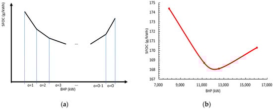
Figure 1. (a) Linear segments o separating the BHP-SFOC curves. (b) The real SFOC data of a ship.

2.2.2. Second Approach

However, the real ship operation may be very different from the new ship condition. Therefore, in the present research, the later historical real ship data were used to approach the realistic condition. The recent hull and machine condition (e.g., fouling condition of the hull) could then be considered in the latest voyage data. Regression analysis was employed to model the relationship between fuel consumption and ship speed based on historical noon report data. These data were categorized according to different BNs, weather directions, loading conditions, and legs. To constrain the scope of the regression analysis, BN and weather direction were selected as the weather variables under consideration. Generally, a higher Beaufort number indicated greater fuel consumption conditions, as shown in Figure 2. The laden condition had a higher fuel consumption curve than the ballast condition, as shown in Figure 3. The weather condition was directly correlated with fuel consumption. The proposed black-box model established the relationship between speed and fuel consumption under different conditions. Additionally, the black-box regression analysis naturally contained the consideration of intermediate parameters such as SFOC, engine loads, and RPM. Furthermore, the current research considered a two-port itinerary, with the loading condition remaining the same for each leg.

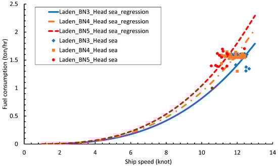
Figure 2. Results of speed–fuel consumption regression for different BNs.

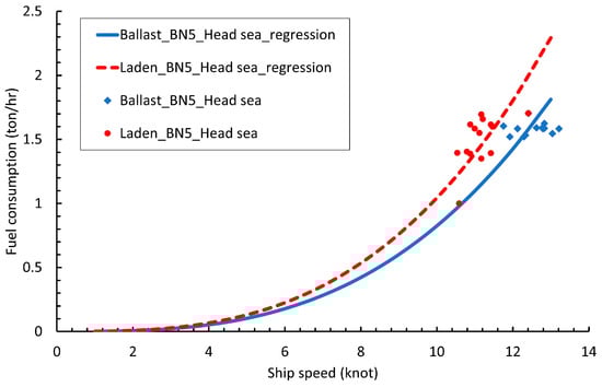
Figure 3. Results of speed–fuel consumption regression for different loading conditions.

The weather direction was derived from relative wind direction and categorized into three directions, that is, head sea, beam sea, and following sea [23,24]. The definition of each weather condition is shown in Figure 4. The regression results of different weather directions are shown in Figure 5. Generally, the fuel consumption of the following sea condition is lower than that of the beam sea and head sea condition, while the fuel consumption of the head sea condition is higher than that of beam sea.

Figure 4. Defined weather directions.

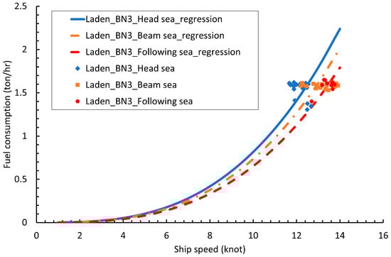
Figure 5. Results of speed–fuel consumption regression for different weather directions.

2.3. Optimization Algorithm

The task of speed optimization for a ship using a single type of fuel is a single-objective optimization problem. In this study, the traditional GA from the pymoo package, developed by Blank and Deb [25], was used to address this problem using Python. Given the potential for daily variations in weather forecasts for each leg of the journey, accuracy is maximized when the optimization procedure is executed at regular intervals [26,27,28]. GA is widely used in a variety of fields [29,30,31,32,33]. The traditional GA consists of six steps: initial population, evaluation, survival, selection, crossover, and mutation. GA comprises two crucial parameters: population size and number of generations, and they directly affect the computational time. Population size is how many sets of solutions are evaluated in one iteration, and number of generations is the maximum iteration. Without enough population size and generations, the optimal solutions may not converge. The flowchart of the proposed method is shown in Figure 6.

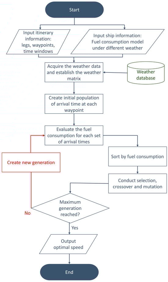
Figure 6. Flowchart of the proposed method.

GA is chosen for its suitability in light of these characteristics, encompassing heuristic, stochastic, and randomized search optimization techniques, all of which are relatively straightforward to describe and implement. In GA, the evaluation is simply calculating the corresponding fitness function of each individual. The selection operator chooses specific individuals for further operation. The crossover operator combines parents to produce the next generation. In mutation, some genes of the individuals were randomly changed on the basis of probability to explore the searching area. Both crossover and mutation operators contain the probability needs to be determined. By properly choosing each operator of GA, the premature convergence may be prevented [34,35]. Thus, the global optimized solution may be obtained.

2.4. Mathematical Model

The sailing time for leg n can be calculated based on the arrival times at waypoints n and n + 1, as formulated in Equation (5). Because the distance for leg n is known, the speed of the ship over ground can be determined, as indicated in Equation (6).

$$t{r}_n=t_{n+1}-t_n \forall n\in N$$

(5)

$$V_n=\frac{D_n}{t{r}_n} \forall n\in N$$

(6)

Weather conditions can be gleaned from forecast data, allowing for the derivation of a weather matrix, presented in Table 2 and formalized in Equations (7) and (8). The columns in this matrix correspond to different arrival times at a waypoint, and the rows represent the waypoints themselves. Each cell in the weather matrix contains the BN and weather direction specific to a given arrival time and waypoint.

$$W_{N\times (M+1)}=\left[\begin{array}{ccccc}{w}_{\mathrm{1,1}}& w_{\mathrm{1,2}}& w_{\mathrm{1,3}}& \cdots & w_{1,\mathrm{M}+1}\\ w_{\mathrm{2,1}}& w_{\mathrm{2,2}}& w_{\mathrm{2,3}}& \cdots & w_{2,\mathrm{M}+1}\\ w_{\mathrm{3,1}}& w_{\mathrm{3,2}}& w_{\mathrm{3,3}}& \cdots & w_{3,\mathrm{M}+1}\\ ⋮& ⋮& ⋮& \ddots & ⋮\\ w_{N,1}& w_{N,2}& w_{N,3}& \cdots & w_{N,\mathrm{M}+1}\end{array}\right]$$

(7)

$$U_{N\times (M+1)}=\left[\begin{array}{ccccc}{u}_{\mathrm{1,1}}& u_{\mathrm{1,2}}& u_{\mathrm{1,3}}& \cdots & u_{1,\mathrm{M}+1}\\ u_{\mathrm{2,1}}& u_{\mathrm{2,2}}& u_{\mathrm{2,3}}& \cdots & u_{2,\mathrm{M}+1}\\ u_{\mathrm{3,1}}& u_{\mathrm{3,2}}& u_{\mathrm{3,3}}& \cdots & u_{3,\mathrm{M}+1}\\ ⋮& ⋮& ⋮& \ddots & ⋮\\ u_{N,1}& u_{N,2}& u_{N,3}& \cdots & u_{N,\mathrm{M}+1}\end{array}\right]$$

(8)

Table 2. Weather matrix for different positions and arrival times.

[Beaufort Number, Weather Direction]	$\mathbf{Waypoint} \mathbf{Arrival} \mathbf{Time}\mathit{t}\mathit{w}$	$\mathbf{Waypoint} \mathbf{Arrival} \mathbf{Time} \mathit{t}\mathit{w}+1$	$\mathbf{Waypoint} \mathbf{Arrival} \mathbf{Time} \mathit{t}\mathit{w}+2$	⋯	$\mathbf{Waypoint} \mathbf{Arrival} \mathbf{Time} \mathit{t}\mathit{w}+\mathit{M}$
Waypoint-1	$[{\mathrm{w}}_{\mathrm{1,1}},u_{\mathrm{1,1}}]$	$[{\mathrm{w}}_{\mathrm{1,2}},u_{\mathrm{1,2}}]$	[${\mathrm{w}}_{\mathrm{1,3}},u_{\mathrm{1,3}}]$	⋯	$[{\mathrm{w}}_{1,\mathrm{M}+1},u_{1,M+1}]$
Waypoint-2	$[{\mathrm{w}}_{\mathrm{2,1}},u_{\mathrm{2,1}}]$	$[{\mathrm{w}}_{\mathrm{2,2}},u_{\mathrm{2,2}}]$	$[{\mathrm{w}}_{\mathrm{2,3}},u_{\mathrm{2,3}}]$	⋯	${[\mathrm{w}}_{2,\mathrm{M}+1},u_{2,M+1}]$
Waypoint-3	${[\mathrm{w}}_{\mathrm{3,1}},{\mathrm{u}}_{\mathrm{3,1}}]$	$[{\mathrm{w}}_{\mathrm{3,2}},u_{\mathrm{3,2}}]$	$[{\mathrm{w}}_{\mathrm{3,3}},u_{\mathrm{3,3}}]$	⋯	$[{\mathrm{w}}_{3,\mathrm{M}+1},u_{3,M+1}]$
$⋮$	$⋮$	$⋮$	$⋮$	$\ddots$	$⋮$
Waypoint-N	$[{\mathrm{w}}_{N,1},u_{N,1}]$	$[{\mathrm{w}}_{N,2},u_{N,2}]$	$[{\mathrm{w}}_{N,3},u_{N,3}]$	⋯	$[{\mathrm{w}}_{N,\mathrm{M}+1},u_{N,M+1}]$

To ensure accurate fuel consumption curves corresponding to the appropriate BN and weather direction, we introduce parameter ${\delta }_{n,s}$ and ${\gamma }_{n,p}$ in Equations (9) and (10), respectively.

$${\delta }_{n,s}=\left\{\begin{array}{c}\begin{array}{cc}1& ,if w_{n,t_n}=s\\ 0& ,otherwise\end{array}\end{array}\right.\forall n\in N, \forall s\in S$$

(9)

$${\gamma }_{n,p}=\left\{\begin{array}{c}\begin{array}{cc}1& ,if u_{n,t_n}=p\\ 0& ,otherwise\end{array}\end{array}\right.\forall n\in N, \forall p\in \mathrm{P}$$

(10)

The constrained optimization problem under consideration can be formally expressed using Equations (11)–(14).

$$\mathrm{x}=[{\mathrm{t}}_1,{\mathrm{t}}_2,\cdots ,{\mathrm{t}}_N]$$

(11)

$$\min FC={\sum }_{n\in N}{\sum }_{s\in S}{\sum }_{p\in P}{(a}_{n,s,p}·V_n^{c_{n,s,p}})·{\delta }_{n,s}·{\mathsf{\gamma }}_{n,p}·{ts}_n$$

(12)

$$\mathrm{s}.\mathrm{t}. tw\le t_n\le tw+M \forall n\in N$$

(13)

$$t_{n+1}-t_n>0$$

(14)

In this model, the variables in Equation (11) refer to the arrival times for each leg of the journey. The objective function in Equation (12) is designed to minimize total fuel consumption. The constraints in Equations (13) and (14) ensure that the arrival time at each port falls within a specified time window and that the arrival time at a subsequent port is later than that of the preceding port, respectively.

3. Results and Discussion

3.1. Case Study

The speed profile and positions of historical sailing mode were obtained by the noon report, and the fuel consumption was simulated by the aforementioned regression analysis. Two different ships and itineraries were demonstrated and showed in this section. The principal dimensions of the target ships are listed in Table 3. By comparing the fuel consumption of optimal speed sailing mode and historical sailing mode, the effect of the proposed optimization process could be estimated. The route maps are shown in Figure 7.

Table 3. Principle dimensions of the target ships.

	Target Ship A	Target Ship B
Length overall (m)	235	300
Breath (m)	38	50
Depth (m)	20	25
Deadweight (ton)	93,000	200,000
Complete year	2011	2013
Operation route	Kaohsiung, Taiwan—Gladstone, Australia	Port Hedland, Australia—Kaoshiung, Taiwan

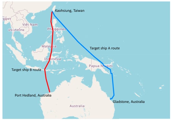
Figure 7. Operation route of target ship A and B.

Binary tournament selection was used in the case studies. The SBX crossover technique was chosen for its good performance in many problems [36]. The crossover probability was 0.5, and the mutation probability was 0.2. The population size was 300, and the maximum number of generations was 300. The optimization problem was computed using a 3.60 GHz 8-Core Intel Core i7 with 32 GB RAM. The calculation time depended on the population and generation size, and amounted to approximately 4.5 min in the case studies.

3.1.1. Case Study 1—93,000 DWT Bulk Carrier

A methodology in a previous study was applied to a 93,000 DWT bulk carrier. The selected itinerary commenced in Kaohsiung of Taiwan and concluded in Gladstone of Australia, passing through the Jomard Entrance and Vitiaz Strait, as detailed in Table 4. The journey spanned 12 days, resulting in 12 distinct legs, with waypoints set at the historical daily noon positions recorded. Time windows for each waypoint were defined as the interval between the departure from the initial port and arrival at the destination, with the total sailing time serving as a fixed boundary condition.

Table 4. Time windows and route in the considered case study 1.

Leg No.	Arrival Port/Waypoint	Acceptable Earliest Arrival Time	Acceptable Latest Arrival Time	Sailing Distance (nm)
	P1-TWKHH	26 May 12:00	26 May 12:00
1	Waypoint 1	26 May 12:00	7 June 10:00	302.00
2	Waypoint 2	26 May 12:00	7 June 10:00	301.00
3	Waypoint 3	26 May 12:00	7 June 10:00	279.00
4	Waypoint 4	26 May 12:00	7 June 10:00	263.00
5	Waypoint 5	26 May 12:00	7 June 10:00	299.00
6	Waypoint 6	26 May 12:00	7 June 10:00	295.00
7	Waypoint 7	26 May 12:00	7 June 10:00	267.00
8	Waypoint 8	26 May 12:00	7 June 10:00	279.00
9	Waypoint 9	26 May 12:00	7 June 10:00	292.00
10	Waypoint 10	26 May 12:00	7 June 10:00	315.00
11	Waypoint 11	26 May 12:00	7 June 10:00	297.00
12	P2-AUGLT	7 June 10:00	7 June 10:00	313.00

The optimization results were subsequently contrasted with the original sailing speed profile, as shown in Table 5.

Table 5. Speed profiles before and after speed optimization for comparison in case study 1.

	Original Sailing Mode				Recommended Sailing Mode
Leg No.	Original Arrival Time (UTC +8)	Original Speed (Knot)	BN	Weather Direction	Recommended Arrival Time (UTC +8)	Recommended Speed (Knot)	BN	Weather Direction
	26 May 12:00	-			26 May 12:00	-	-
1	27 May 12:00	12.58	4	Beam sea	27 May 13:02	12.07	4	Beam sea
2	28 May 12:00	12.54	4	Following sea	28 May 12:57	12.58	4	Following sea
3	29 May 11:00	12.13	4	Following sea	29 May 11:10	12.58	4	Following sea
4	30 May 11:00	10.96	5	Beam sea	30 May 08:57	12.08	4	Beam sea
5	31 May 11:00	12.46	3	Beam sea	31 May 09:35	12.15	3	Beam sea
6	1 June 11:00	12.29	3	Beam sea	1 June 09:51	12.15	3	Beam sea
7	2 June 10:00	11.61	4	Beam sea	2 June 07:56	12.08	4	Beam sea
8	3 June 10:00	11.63	5	Beam sea	3 June 06:59	12.08	4	Beam sea
9	4 June 10:00	12.17	3	Beam sea	4 June 06:05	12.65	3	Following sea
10	5 June 10:00	13.13	3	Beam sea	5 June 06:59	12.65	3	Following sea
11	6 June 10:00	12.38	3	Beam sea	6 June 06:59	12.38	3	Following sea
12	7 June 10:00	13.04	4	Beam sea	7 June 10:00	11.59	4	Beam sea
Oil consumption (ton)	291.17				280.63
difference					−3.6%

Data from Table 5 indicate that the proposed model succeeded in lowering oil consumption. In legs 4, 8, 9, 10, and 11, the optimized arrival time corresponded with periods of lower BN and following sea condition, thereby reducing resistance and conserving fuel. Under the constraint of fixed voyage time, the average speeds for both the original and optimized sailing modes remained identical. Moreover, the range between the highest and lowest speeds in the recommended sailing mode exceeded that in the original sailing mode.

This study employed a daily time period for optimization. If higher-frequency historical voyage data become available, the use of a finer temporal resolution could produce more realistic conditions for optimization.

3.1.2. Case Study 2—200,000 DWT Bulk Carrier

Similarly, the methodology was then applied on a 200,000 DWT bulk carrier. The itinerary details are listed in Table 6. The selected itinerary commenced in Port Hedland of Australia and concluded in Kaohsiung of Taiwan. The optimization results are listed in Table 7. The results similarly indicated that the proposed method can effectively avoid the encountered harsh weather condition in legs 1, 4, and 5 and reduce total fuel consumption.

Table 6. Time windows and route in the considered case study 2.

Leg No.	Arrival Position	Acceptable Earliest Arrival Time	Acceptable Latest Arrival Time	Sailing Distance (nm)
	P1-AUPHE	29 October 12:00	29 October 12:00
1	Waypoint 1	29 October 12:00	7 November 12:00	286
2	Waypoint 2	29 October 12:00	7 November 12:00	295
3	Waypoint 3	29 October 12:00	7 November 12:00	296
4	Waypoint 4	29 October 12:00	7 November 12:00	281
5	Waypoint 5	29 October 12:00	7 November 12:00	298
6	Waypoint 6	29 October 12:00	7 November 12:00	264
7	Waypoint 7	29 October 12:00	7 November 12:00	277
8	Waypoint 8	29 October 12:00	7 November 12:00	276
9	P2-TWKHH	7 November 12:00	7 November 12:00	248

Table 7. Speed profiles before and after speed optimization for comparison in case study 2.

	Original Sailing Mode				Recommended Sailing Mode
Leg No.	Original Arrival Time (UTC +8)	Original Speed (Knot)	BN	Weather Direction	Recommended Arrival Time (UTC +8)	Recommended Speed (Knot)	BN	Weather Direction
	29 October 12:00	-			29 October 12:00
1	30 October 12:00	11.92	4	Beam sea	30 October 10:59	12.44	3	Beam sea
2	31 October 12:00	12.29	4	Following sea	31 October 12:32	11.55	4	Following sea
3	1 November 12:00	12.33	3	Following sea	1 November 13:53	11.67	3	Following sea
4	2 November 12:00	11.71	3	Beam sea	2 November 15:59	10.77	2	Beam sea
5	3 November 12:00	12.42	3	Head sea	3 November 20:00	10.64	3	Beam sea
6	4 November 12:00	11.0	4	Beam sea	4 November 18:17	11.84	4	Beam sea
7	5 November 12:00	11.54	3	Beam sea	5 November 17:25	11.98	3	Beam sea
8	6 November 12:00	11.50	4	Following sea	6 November 14:45	12.93	4	Following sea
9	7 November 12:00	10.33	7	Beam sea	7 November 12:00	11.68	7	Beam sea
Oil consumption (ton)	347.42				338.68
difference					−2.5%

3.2. Sensitivity Analysis

To validate the proposed model, the sensitivity analysis for target ship A and the itinerary between Kaohsiung and Gladstone was conducted. In Section 3.2.1, the different BN-affected speed–fuel consumption curves are discussed. In Section 3.2.2, the different weather direction-affected speed–fuel consumption curves are discussed. In Section 3.2.3, the effects of different total sailing time are investigated.

3.2.1. Effects of Different BN-Affected Speed–Fuel Consumption Curves

Through the model establishment Equations (1)–(12) and case studies, the speed–fuel consumption curves proved to be critical in the optimization model. As we discussed in Section 2.2, the speed–fuel consumption curves could be derived by the sea trial test. However, the realistic condition may be different from the sea trial condition, and may be obtained by the regression of the later historical voyage data. Thus, the speed–fuel consumption curves were directly set in this section to simulate the regression of historical data. To separate the effects of BN and weather direction, the weather direction was considered no influence on the speed–fuel consumption curves in this section.

To investigate the effects of different fuel consumption curves, four scenarios—designated as Scenario 1 through Scenario 4—were established to represent different effects of the Beaufort scale on fuel usage. Scenario 1 posited that the Beaufort scale had no influence on oil consumption. Conversely, Scenarios 2, 3, and 4 indicated that a single unit increase in the BN would result in a 2%, 4%, and 6%, rise in fuel consumption, respectively. The fuel consumption parameter $a_s$ for the different BNs are listed in Table 8, with $c_s$ consistently fixed at 3. In other words, the fuel consumption curves in Scenarios 1–4 follow the formula $a_s·V^3$. The set fuel consumption curves for each scenario are shown in Figure 8. Therefore, all the curves in Figure 8 are cubic. By comparing the optimal speed of Scenario 1 and the theoretical optimal speed profile (average speed), the optimization process could be validated. By comparing the optimal speed of Scenario 1, 2, 3, and 4, the effects of different BN-affected oil consumption curves could be evaluated.

Table 8. Setting fuel consumption parameter $a_s$ in different scenarios.

${\mathit{a}}_{\mathit{s}}$	Scenario 1	Scenario 2	Scenario 3	Scenario 4
BN = 2	0.0004370 (+0%)	0.0004195 (−4%)	0.0004020 (−8%)	0.0003846 (−12%)
BN = 3	0.0004370 (+0%)	0.0004283 (−2%)	0.0004195 (−4%)	0.0004108 (−6%)
BN = 4	0.0004370 (+0%)	0.0004370 (+0%)	0.0004370 (+0%)	0.0004370 (+0%)
BN = 5	0.0004370 (+0%)	0.0004457 (+2%)	0.0004545 (+4%)	0.0004632 (+6%)
BN = 6	0.0004370 (+0%)	0.0004545 (+4%)	0.0004720 (+8%)	0.0004894 (+12%)

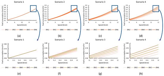
Figure 8. Four scenarios for investigating the effects of different speed–fuel consumption curves corresponding to different BNs. The darker line corresponds to a bigger BN. (a) Scenario 1, (b) Scenario 2, (c) Scenario 3, and (d) Scenario 4. A closer look is shown in (e–h). (e) Scenario 1, (f) Scenario 2, (g) Scenario 3, and (h) Scenario 4.

The optimization results are presented in Table 9 and visualized in Figure 9. For Scenarios 2, 3, and 4, the optimal solutions indicated that ships ought to have a higher and lower speed during adverse and favorable weather conditions, respectively. Specifically, optimal speeds in Scenario 2, 3, and 4 led to a lower BN in leg 8 compared with that in Scenario 1. In Scenario 1, an average speed was proposed, given that the same fuel consumption parameter remained constant across different BNs. The proposed method is validated by comparing the theoretical best speed (i.e., the average speed) with the optimized speed. The slight difference between Scenario 1 and theoretical average speed was due to the fact that GA can only obtain the approximate optimal solution. As the disparity in Beaufort number increased from Scenario 2 to Scenario 4, the difference between the highest and lowest recommended speeds widened. This suggests that decreasing speed during adverse weather conditions and increasing speed during more favorable weather yield greater advantages when adverse conditions substantially increase oil consumption. Furthermore, Scenario 4 obtained a lower BN in leg 1 than those in Scenario 2 and 3. This shows that if the lower BN can only be obtained by adjusting the speed profile a lot, GA will determine whether it is worthy to adjust. In this case, it was not worthy to adjust it for the fuel consumption curves of Scenario 2 and 3, but the fuel consumption curves of different BNs were different enough for the optimal speed to adjust more in Scenario 4.

Table 9. Optimization results for different scenarios.

	Scenario 1		Scenario 2		Scenario 3		Scenario 4
Leg No.	Speed (Knot)	BN	Speed (Knot)	BN	Speed (Knot)	BN	Speed (Knot)	BN
1	12.26	4	12.21	4	12.3	4	11.19	3
2	12.26	4	12.21	4	12.31	4	12.58	4
3	12.25	4	12.2	4	12.29	4	12.58	4
4	12.25	4	12.2	4	12.18	4	12.58	4
5	12.25	3	12.29	3	12.39	3	12.42	3
6	12.24	3	12.29	3	12.4	3	12.4	3
7	12.24	4	12.2	4	12.19	4	12.11	4
8	12.24	5	12.2	4	12.11	4	12.1	4
9	12.24	3	12.31	3	12.27	3	12.39	3
10	12.24	3	12.31	3	12.25	3	12.37	3
11	12.24	3	12.31	3	12.26	3	12.36	3
12	12.24	4	12.21	4	12.01	4	12.05	4

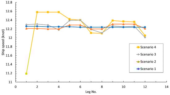
Figure 9. Optimal speeds (blue circle, orange triangle, grey diamond, yellow square) representing Scenario 1, Scenario 2, Scenario 3, and Scenario 4, respectively.

3.2.2. Effects of Different Weather Direction-Affected Speed–Fuel Consumption Curves

In this subsection, the effects of different weather direction-affected speed–fuel consumption curves were investigated, and the BN was assumed to have no influence on fuel consumption. Similarly, three scenarios were set to represent different weather direction effects. Scenario 5 posited that the weather direction had no influence on fuel consumption. Scenario 6 and 7 represented the fuel consumption of head sea condition being higher than that of beam sea condition by 1% and 2%, respectively. On the other hand, Scenario 6 and 7 were set so that the fuel consumption of following sea condition was lower than that of beam sea condition by 1% and 2%, respectively. The fuel consumption parameter $a_p$ for the different weather directions are listed in Table 10, with $c_p$ consistently fixed at 3. In other words, the fuel consumption curves in Scenarios 5–7 follow the formula $a_p·V^3$. By comparing the optimal speed of Scenario 5 and the average speed, the optimization process could be validated. By comparing the optimal speed of Scenario 5, 6, and 7, the effects of different weather direction-affected oil consumption curves could be evaluated.

Table 10. Setting fuel consumption parameter $a_p$ in different weather direction scenarios.

${\mathit{a}}_{\mathit{p}}$	Scenario 5	Scenario 6	Scenario 7
Head sea	0.0004370 (+0%)	0.0004414 (+1%)	0.0004457 (+2%)
Beam sea	0.0004370 (+0%)	0.0004370 (+0%)	0.0004370 (+0%)
Following sea	0.0004370 (+0%)	0.0004326 (−1%)	0.0004283 (−2%)

The optimal speed of Scenarios 5 to 7 was shown in Table 11 and Figure 10. Similarly, the optimal speed of Scenario 5 is slightly different from the theoretical optimal average speed, because of the nature of GA. In Scenarios 6 and 7, the optimal speed is sailing faster in lower fuel consumption condition, that is, the following sea condition. The gap between the maximum and minimum speed of Scenario 7 is larger than that of Scenario 6 because of the larger difference in the fuel consumption curves in Scenario 7.

Table 11. Optimization results for different weather direction scenarios.

	Scenario 5		Scenario 6		Scenario 7
Leg No.	Speed (Knot)	Weather Direction	Speed (Knot)	Weather Direction	Speed (Knot)	Weather Direction
1	12.26	Beam sea	12.27	Beam sea	12.21	Beam sea
2	12.26	Following sea	12.31	Following sea	12.31	Following sea
3	12.25	Following sea	12.31	Following sea	12.31	Following sea
4	12.25	Beam sea	12.25	Beam sea	12.23	Beam sea
5	12.25	Beam sea	12.25	Beam sea	12.24	Beam sea
6	12.24	Beam sea	12.25	Beam sea	12.25	Beam sea
7	12.24	Beam sea	12.25	Beam sea	12.25	Beam sea
8	12.24	Beam sea	12.25	Beam sea	12.26	Beam sea
9	12.24	Following sea	12.3	Following sea	12.36	Following sea
10	12.24	Beam sea	12.6	Following sea	12.6	Following sea
11	12.24	Beam sea	12.37	Following sea	12.37	Following sea
12	12.24	Beam sea	11.59	Beam sea	11.59	Beam sea

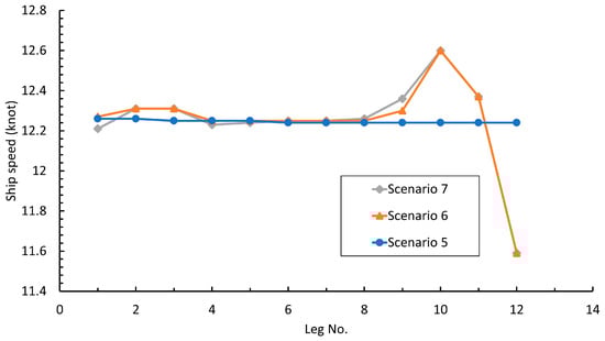
Figure 10. Optimal speeds (blue circle, orange triangle, grey diamond) representing Scenario 5, Scenario 6, and Scenario 7, respectively.

3.2.3. Effects of Different Total Sailing Time

This study also investigated the fuel consumption associated with different total sailing times. The accuracy of these results is directly affected by the fuel consumption curves, which can be further refined with high-frequency raw data. The itinerary commenced on 26 May at 12:00 and concluded at various times: 6 June at 18:00, 7 June at 02:00, 7 June at 10:00, 7 June at 18:00, and 8 June at 02:00, as detailed in Table 12. As expected, fuel consumption was higher at shorter sailing times. However, reducing the total sailing time led to a more pronounced increase in fuel consumption than the fuel savings achieved by extending the total sailing time by an equivalent duration. This phenomenon aligns well with the nonlinear nature of fuel consumption curves. Specifically, increasing speed led to a more substantial rise in fuel consumption than the corresponding reduction achieved by a similar decrease in speed. Practically, slow steaming may cause other issues. In the low-load condition, the unburned fuel and lubricating oil may accumulate in the exhaust pipes. These carbon deposits could be cleaned by periodically increasing the main engine back to the high-load condition [37].

Table 12. Optimization results for different itinerary end times.

Itinerary End Time	Total Sailing Time (h)	Fuel Consumption (ton)
6 June 18:00	270 (−5.6%)	287.65 (+2.5%)
7 June 02:00	278 (−2.8%)	283.16 (+0.9%)
7 June 10:00	286 (+0%)	280.63 (+0%)
7 June 18:00	294 (+2.8%)	278.38 (−0.8%)
8 June 02:00	302 (+5.6%)	276.14 (−1.6%)

4. Conclusions and Prospects

This study introduced a speed optimization model tailored for two-port bulk carrier routes, incorporating weather conditions along the route. Using GA for problem-solving, the model estimated fuel consumption through regression analysis of historical noon reports. In this study, the different weather conditions of different time at the same location were considered, and the weather matrix was established in the mathematical model. The proposed method could effectively reduce fuel consumption by around 2–3%, as evidenced by the case study. Generally, the optimal speed recommendation suggested that the ship should sail at a higher speed under conditions of lower fuel consumption, such as lower BN and following sea conditions. However, if lower fuel consumption conditions could be achieved by adjusting the speed, the GA would determine whether it was worthwhile to pursue. Subsequently, this study conducted sensitivity analyses of different weather affected fuel consumption curves. The findings indicated that for ships whose fuel consumption is highly sensitive to BNs or weather directions, speed adjustments based on weather conditions become critical for maintaining energy efficiency. Given that bulk carriers often lack strict arrival time constraints at their finals, the study also explored the relationship between arrival time and fuel consumption. Consistent with other studies, reduced speed is correlated with lower fuel consumption. The model was also validated by comparing the theoretical optimal speed of Scenario 1 and 5 with the optimized speed in these sensitivity analyses. The accuracy of the proposed optimization model hinges on two primary factors: the reliability of weather forecasts, and the precision of fuel consumption estimates. By considering more factors and higher-frequency data, the fuel consumption model may be more realistic. On the other hand, although slow steaming can effectively reduce fuel cost and carbon emissions, the profits and other costs of the ship may be affected. This practical trade-off can be considered to determine the best sailing mode. While the present research focuses on bulk carriers, different ship types may also be considered in the future. Future work could potentially focus on refining these aspects to further enhance the model’s effectiveness.

The future research aspects can also be carried out by applying different optimization algorithms such as particle swarm optimization (PSO) and ant colony optimization (ACO) on the proposed model. The most effective and suitable algorithm of the problem can then be assessed by comparing the obtained results and consumed resources.

References

- IMO. Resolution MEPC.377(80), 2023 IMO Strategy on Reduction of GHG Emissions from Ships; International Maritime Organization: London, UK, 2023. [Google Scholar]
- Fagerholt, K.; Laporte, G.; Norstad, I. Reducing fuel emissions by optimizing speed on shipping routes. J. Oper. Res. Soc. 2010, 61, 523–529. [Google Scholar] [CrossRef]
- Gao, C.-F.; Hu, Z.-H. Speed Optimization for Container Ship Fleet Deployment Considering Fuel Consumption. Sustainability 2021, 13, 5242. [Google Scholar] [CrossRef]
- Lu, J.; Wu, X.; Wu, Y. The Construction and Application of Dual-Objective Optimal Speed Model of Liners in a Changing Climate: Taking Yang Ming Route as an Example. J. Mar. Sci. Eng. 2023, 11, 157. [Google Scholar] [CrossRef]
- Shih, Y.-C.; Tzeng, Y.-A.; Cheng, C.-W.; Huang, C.-H. Speed and Fuel Ratio Optimization for a Dual-Fuel Ship to Minimize Its Carbon Emissions and Cost. J. Mar. Sci. Eng. 2023, 11, 758. [Google Scholar] [CrossRef]
- Wang, Z.; Fan, A.; Tu, X.; Vladimir, N. An energy efficiency practice for coastal bulk carrier: Speed decision and benefit analysis. Reg. Stud. Mar. Sci. 2021, 47, 101988. [Google Scholar] [CrossRef]
- Li, X.; Sun, B.; Guo, C.; Du, W.; Li, Y. Speed optimization of a container ship on a given route considering voluntary speed loss and emissions. Appl. Ocean Res. 2020, 94, 101995. [Google Scholar] [CrossRef]
- Yang, L.; Chen, G.; Zhao, J.; Rytter, N.G.M. Ship Speed Optimization Considering Ocean Currents to Enhance Environmental Sustainability in Maritime Shipping. Sustainability 2020, 12, 3649. [Google Scholar] [CrossRef]
- Zhuge, D.; Wang, S.; Wang, D.Z.W. A joint liner ship path, speed and deployment problem under emission reduction measures. Transp. Res. Part B Methodol. 2021, 144, 155–173. [Google Scholar] [CrossRef]
- Ballou, P.; Henry, C.; John, D. Horner, Advanced Methods of Optimizing Ship Operations to Reduce Emissions Detrimental to Climate Change. In Proceedings of the Oceans 2008, Quebec City, QC, Canada, 15–18 September 2008; pp. 1–12. [Google Scholar] [CrossRef]
- Song, S.; Demirel, Y.K.; Atlar, M.; Dai, S.; Day, S.; Turan, O. Validation of the CFD approach for modelling roughness effect on ship resistance. Ocean Eng. 2020, 200, 107029. [Google Scholar] [CrossRef]
- Chirosca, A.-M.; Medina, A.; Pacuraru, F.; Saettone, S.; Rusu, L.; Pacuraru, S. Experimental and Numerical Investigation of the Added Resistance in Regular Head Waves for the DTC Hull. J. Mar. Sci. Eng. 2023, 11, 852. [Google Scholar] [CrossRef]
- Tadros, M.; Ventura, M.; Guedes Soares, C. Effect of Hull and Propeller Roughness during the Assessment of Ship Fuel Consumption. J. Mar. Sci. Eng. 2023, 11, 784. [Google Scholar] [CrossRef]
- Kwon, Y.J. Speed loss due to added resistance in wind and waves. Nav. Archit. 2008, 3, 14–16. [Google Scholar]
- Kuroda, M.; Tsujimoto, M.; Fujiwara, T.; Ohmatsu, S.; Takagi, K. Investigation on components of added resistance in short waves. J. Jpn. Soc. Nav. Archit. Ocean Eng. 2008, 8, 171–176. [Google Scholar] [CrossRef]
- Lu, R.; Turan, O.; Boulougouris, E.; Banks, C.; Incecik, A. A semi-empirical ship operational performance prediction model for voyage optimization towards energy efficient shipping. Ocean Eng. 2015, 110, 18–28. [Google Scholar] [CrossRef]
- Kim, K.J.; Lee, S.D.; Jun, C.H.; Park, K.M.; Byeon, S.S. A statistical procedure of analyzing container ship operation data for finding fuel consumption patterns. Korean J. Appl. Stat. 2017, 30, 633–645. [Google Scholar] [CrossRef]
- Adland, R.; Cariou, P.; Wolff, F.-C. Optimal ship speed and the cubic law revisited: Empirical evidence from an oil tanker fleet. Transp. Res. Part E Logist. Transp. Rev. 2020, 140, 101972. [Google Scholar] [CrossRef]
- Wang, S.; Ji, B.; Zhao, J.; Liu, W.; Xu, T. Predicting ship fuel consumption based on LASSO regression. Transp. Res. Part D Transp. Environ. 2018, 65, 817–824. [Google Scholar] [CrossRef]
- Karagiannidis, P.; Themelis, N.; Zaraphonitis, G.; Spandonidis, C.; Giordamlis, C. Ship Fuel Consumption Prediction using Artificial Neural Networks. In Proceedings of the Annual Meeting of Marine Technology Conference Proceedings, Athens, Greece, 26 November 2019; pp. 46–51. [Google Scholar]
- Kim, Y.-R.; Jung, M.; Park, J.-B. Development of a Fuel Consumption Prediction Model Based on Machine Learning Using Ship In-Service Data. J. Mar. Sci. Eng. 2021, 9, 137. [Google Scholar] [CrossRef]
- Beşikçi, E.B.; Arslan, O.; Turan, O.; Ölçer, A.I. An artificial neural network based decision support system for energy efficient ship operations. Comput. Oper. Res. 2016, 66, 393–401. [Google Scholar] [CrossRef]
- Blendermann, W. Parameter identification of wind loads on ships. J. Wind. Eng. Ind. Aerodyn. 1994, 51, 339–351. [Google Scholar] [CrossRef]
- Bialystocki, N.; Konovessis, D. On the estimation of ship’s fuel consumption and speed curve: A statistical approach. J. Ocean Eng. Sci. 2016, 1, 157–166. [Google Scholar] [CrossRef]
- Blank, J.; Deb, K. Pymoo: Multi-Objective Optimization in Python. IEEE Access 2020, 8, 89497–89509. [Google Scholar] [CrossRef]
- Tzortzis, G.; Sakalis, G. A dynamic ship speed optimization method with time horizon segmentation. Ocean Eng. 2021, 226, 108840–108853. [Google Scholar] [CrossRef]
- Vettor, R.; Bergamini, G.; Guedes Soares, C. A Comprehensive Approach to Account for Weather Uncertainties in Ship Route Optimization. J. Mar. Sci. Eng. 2021, 9, 1434. [Google Scholar] [CrossRef]
- Vettor, R.; Soares, C.G. Reflecting the uncertainties of ensemble weather forecasts on the predictions of ship fuel consumption. Ocean Eng. 2021, 250, 111009. [Google Scholar] [CrossRef]
- Weile, D.S.; Michielssen, E. Genetic algorithm optimization applied to electromagnetics: A review. IEEE Trans. Antennas Propag. 1997, 45, 343–353. [Google Scholar] [CrossRef]
- Cus, F.; Balic, J. Optimization of cutting process by GA approach. Robot. Comput.-Integr. Manuf. 2003, 19, 113–121. [Google Scholar] [CrossRef]
- Fernandez, M.; Caballero, J.; Fernandez, L.; Sarai, A. Genetic algorithm optimization in drug design QSAR: Bayesian-regularized genetic neural networks (BRGNN) and genetic algorithm-optimized support vectors machines (GA-SVM). Mol. Divers. 2011, 15, 269–289. [Google Scholar] [CrossRef]
- Johnson, J.M.; Rahmat-Samii, Y. Genetic algorithm optimization and its application to antenna design. In Proceedings of the IEEE Antennas and Propagation Society International Symposium and URSI National Radio Science Meeting, Seattle, WA, USA, 20–24 June 1994; pp. 326–329. [Google Scholar]
- Abdelmegid, M.A.; Shawki, K.M.; Abdel-Khalek, H. GA optimization model for solving tower crane location problem in construction sites. Alex. Eng. J. 2015, 54, 519–526. [Google Scholar] [CrossRef]
- Fitzgerald, J.; Wong-Lin, K. Multi-objective optimisation of cortical spiking neural networks with genetic algorithms. In Proceedings of the 2021 32nd Irish Signals and Systems Conference (ISSC), Athlone, Ireland, 10–11 June 2021; pp. 1–6. [Google Scholar]
- Khan, A.; Deb, K. Optimizing Keyboard Configuration Using Single and Multi-Objective Evolutionary Algorithms. In Proceedings of the Companion Conference on Genetic and Evolutionary Computation, Lisbon, Portugal, 24 July 2023; pp. 219–222. [Google Scholar]
- Deb, K.; Sindhya, K.; Okabe, T. Self-adaptive simulated binary crossover for real-parameter optimization. In Proceedings of the 9th Annual Conference on Genetic and Evolutionary Computation, GECCO ’07, New York, NY, USA, 7–11 July 2007; pp. 1187–1194. [Google Scholar] [CrossRef]
- Wiesmann, A. Slow steaming—A viable long-term option. Wartsila Tech. J. 2010, 2, 49–55. [Google Scholar]
Disclaimer/Publisher’s Note: The statements, opinions and data contained in all publications are solely those of the individual author(s) and contributor(s) and not of MDPI and/or the editor(s). MDPI and/or the editor(s) disclaim responsibility for any injury to people or property resulting from any ideas, methods, instructions or products referred to in the content. |
© 2023 by the authors. Licensee MDPI, Basel, Switzerland. This article is an open access article distributed under the terms and conditions of the Creative Commons Attribution (CC BY) license (https://creativecommons.org/licenses/by/4.0/).