1. Introduction
Regular inspection of the condition of various underwater utility lines and pipeline structures such as gas and oil pipelines, as well as cables providing communication and power supply, is an important practical issue to date. Initially, such inspection operations were carried out by divers; subsequently, remotely operated underwater vehicles (ROV) began to be used for these purposes. Today, the deployment of autonomous underwater vehicles (AUV) for inspection purposes is more efficient and cost effective because in this case, the time of operation is reduced, as well as the lease terms of supporting vessels. Furthermore, AUVs provide an opportunity to inspect communications in polar regions and in winter, when access from the surface may be limited by the sea ice cover.
In many cases, the inspection of underwater utility lines is performed in two stages. At the first stage, a broadband reconnaissance survey is carried out along the utility line route in order to evaluate the general condition of both the structure and the adjacent bottom surface, as well as to search for foreign objects. At this stage, acoustic means are usually used that provide a sufficient range of object detection and a wide field of view (side-scanning, sector-scanning, or forward-looking sonars). The algorithms for identifying and determining the characteristics of local and continuous on-bottom objects in sonar scan images, as well as the organization of an AUV’s approach to these objects, are quite well developed (for example, in [
1,
2]).
At the second stage, the object proper is inspected. The use of AUVs in this case requires two main problems to be solved: the accurate localization of the AUV relative to the object in order to provide the precision navigation referencing of the defects found, and the organization of tracing of the utility lines laid on the seabed. Many developers and teams of companies specialized, in particular, in pipeline inspection activities make efforts to address these issues. Almost all studies focus on the integration of various sensors for improving the accuracy and reliability of AUV’s movement along underwater pipeline (UP). The main set of sensors includes laser systems with various scanning modes, a bottom profiler, a magnetometer, and auxiliary sensors (GeoChemical suite of sensors, etc.). A digital video camera is also always used, usually in the 2D image capture mode.
Note that, to date, the methods and algorithms for recognizing objects from images have been well developed mostly for ground-based scenarios. But these are not always suitable for the underwater environment due to the specific photographing conditions such as poor illumination, turbidity of water, water currents, possible interference in the form of fouling of the object by algae and shellfish, sediment cover, or accumulations of debris along the UP. Thus, the range of problems associated with the organization of this stage of UP inspection cannot yet be considered fully addressed. Further development of relevant technologies is required to be focused, in particular, on the detection and tracking of UPs with AUVs.
Related Studies
Various approaches based on the processing of sonar, laser, and optical information have been used to address the issue of UP recognition with AUV in recent years. Major attention has been paid to both specific aspects of the problem and the integration of various types of sensor-derived data.
A lot of works has been devoted to the use of sonar for UP tracking, since the approach based on the processing of sonar information has long been proven to be an effective tool for underwater research. In particular, it allows one to obtain a detailed picture of the underwater scene, regardless of the purity of the water. For example, the study [
3] proposes a technique for UP identification in sonar images through suppression of the speckle noise, analysis of pixels belonging to the pipeline, and application of the coarse segmentation method. In the study [
4], the use of a forward-looking sonar to reduce the accumulation of errors in the integrated navigation system of the vehicle (with a multibeam sonar system) over a long period of operation is considered. To provide such a mode of operation, a tracking algorithm is proposed. The study [
5] proposes an automatic cable-tracking method based on side-scan sonar that endows AUVs with autonomous decision-making capabilities to achieve fast localization and stable tracking of submarine cables with large uncertainties. When a cable is detected, the cable-tracking task is constructed as a path-following control problem on the horizontal plane.
A frequently used and justified approach to pipeline tracking is the use of sensor combinations, since this increases the reliability of object recognition and the information content of the inspection. The paper [
6] shows the preliminary perceptions of pipeline inspection with AUV in oil and gas fields. The intent of this new technology is to increase productivity and reduce costs related to facilities inspection. The AUV used is a Kongsberg HUGIN 1000 equipped with a synthetic aperture sonar, a multibeam echosounder, a Doppler velocity long, differential global navigation satellite systems, a hydrocarbon sensor, an inertial navigation system, a high-definition camera, and a turbidity sensor. In the inspection, it is possible to identify the integrity level of the pipeline as well as the environmental conditions of its surroundings, such as: damage, wreckage, buried or partially buried sectors, free-spans, carbonate sediments, pipeline crossings, and buckling. In [
7,
8], the authors propose a technique to control an underwater vehicle based on combination of data from various sensors, including a camera, a multibeam echosounder, a seabed profiler, and a magnetic sensor. The algorithms for combining data and recognizing pipelines/cables utilize probabilistic maps that contain information about the location and rating of data received from each sensor. The technique for controlling an underwater vehicle is also described as follows: waypoints are generated for the AUV to move at a specified distance from the target object. The study [
9] proposes the ocean floor geophysics (OFG) AUV non-contact integrated cathodic protection (iCP) inspection system based on electric field measurements. When combined with the camera imaging, multi-beam measurements, synthetic aperture sonar (HISAS), and chemical sensors, the OFG AUV iCP system provides a compelling set of measurements for monitoring the pipeline cathodic protection and pipeline inspection.
A promising approach today is the use of learning methods using neural networks. For example, the paper [
10] presents a method for locating and detecting objects in an underwater image based on the multi-scale covariance descriptor and the support vector machine classifier. The features used for image description are well selected in order to be suitable to describe the object sought. The descriptor parameters are adapted for the underwater context. The detection results are compared to the mono-scale description using a covariance descriptor. The proposed method has been successfully tested for underwater pipe detection on the Maris dataset (MARIS Italian national project). Recently, due to the improvement of the deep convolutional network technology, neural networks have been actively used to address the problems of detection and automatic tracking of UP and cables. For example, in the studies [
11,
12,
13,
14], the authors analyze various aspects of efficiency of their application, including such issues as selection of a neural network architecture and its training, computational efficiency, and reliability of recognition when applied in the underwater environment. This includes deploying a deep neural network to recognize pipes and valves in multiple underwater scenarios using 3D RGB point cloud information from a stereo camera.
To a relatively lesser extent, attention has been paid to UP inspection methods with the use of only visual information or predominant use of visual information. Noteworthy in this sense was the work [
15]. A vision system for real-time, underwater cable tracking was presented. Using only visual information, the system is able to locate and follow a cable in an image sequence, overcoming the typical difficulties of underwater scenes. The cable-tracking strategy is based on the hypothesis that the cable parameters are not going to change too much from one image to the next. We note two things here. First—in this work, only a 2D solution for cable tracking is obtained, which is not enough when it is necessary to determine the relative position in 3D space of AUVs and Ups when performing inspection and repair operations. Second—we note that in our work, we also applied the tracking strategy of “minor change in parameters”, but not with respect to neighboring images, but to the calculation of the UP centerline in 3D space. The article [
16] is interesting in that it gives a comparative analysis of vision-based systems used for detection and tracking of cables/pipelines laid in the seabed. A brief review of previous work is also given here. The authors note that most of all feature-based methods use edge features for detecting cable/pipeline borders. And for extracting out the lines representing contours, Hough transform [
17] is the ever-favorite option [
18]. In the study [
19], the authors present a method for pipeline localization relative to the AUV in 3D based on the stereo vision and depth data from echosounder. The angle of pipeline inclination and the seabed are assumed to be close to horizontal, and the pipeline to constitute a straight line. The pipeline is segmented out in the camera images by thresholding using the Otsu’s method [
20] and is eroded in order to remove noise objects in the image, before the edges are found using a Sobel filter. The pipeline is detected as a centerline in the middle of these. In the study [
21], the problem of AUV following down a UP was addressed using images taken with an optical mono-camera. In the images, visible UP boundary lines, used by the control system as feedback when controlling AUV’s movements, are highlighted by the Hough algorithm. In the study [
22], the design of a visual control scheme aimed at solving a pipeline tracking control problem is discussed. The presented scheme consists in autonomously generating a reference path of an underwater pipeline deployed on the seabed from the images taken with a camera mounted on the AUV in order to allow the vehicle to move parallel to the longitudinal axis of the pipeline so as to inspect its condition.
The paper [
23] reviews the latest advances in integrated navigation technologies for AUVs aimed to create inertial navigation systems with auxiliary sensors to improve the navigation accuracy of inertial sensors for AUVs.
The review [
24] covers the most frequently used subsea inspection and monitoring technologies, as well as their most recent advances and future trends.
In general, an analysis of the above-mentioned and other well-known publications that dealt with optical image processing has shown that the issue of UP detection and tracking from optical images is solved, as a rule, using different versions of the Canny detector [
25] for edge detection and the Hough transform for detecting lines from source images. Image processing is often integrated with measurements by other sensors. We should note, however, that the potential of 3D information derived from optical images is not yet fully utilized for addressing problems of detection and tracking of UP (or other linear objects). In particular, tracking a UP requires different algorithmic supports for the continuous tracking mode and the local recognition mode (recognition at the initial moment of inspection or immediately beyond the UP segment hidden by various objects such as sand, algae, etc.). A more efficient use of a vectorized form of source images is possible, which expands the algorithmic capabilities. Of certain interest is also the development of algorithms that provide an alternative to the computation-consuming Hough transform method. With them, the restriction relative to the plane of the seabed topography is not mandatory. Therefore, the technologies based on optical image processing need further development.
The present article aimed to solve the problem of UP recognition and tracking with AUV in the context of addressing the issue of inspection of continuous linear objects underwater. The focus was on a more efficient utilization of the potential of stereo images taken with AUV’s camera. A contribution of this study consists in the development of a new approach to solving this problem through highlighting of visible UP boundaries and calculation of the UP centerline using algorithms for combined processing of 2D and 3D video data. The proposed method is based on the software and algorithmic tools previously developed by the authors [
26]. The technology proposed may be of practical use in the development of navigation systems to be applied to UP inspection without deploying additional, expensive equipment. However, this does not rule out its use in combination with measurements by other sensors. The efficiency of the algorithms was assessed in the environment of a modeling system (underwater robotics simulator) developed by the authors [
27], as well as using actual underwater photography data obtained from an AUV.
2. Problem Setting
The problem of recognition and tracking of an underwater pipeline (UP) is solved using a video stream recorded with a stereo camera installed on board an autonomous underwater vehicle (AUV). For this, assume that
the UP lies on the seabed surface and reproduces features of the bottom topography, i.e., the direction changes in 3D space;
the UP diameter is known;
the UP (cylinder) boundary that the camera sees from certain position is one of the generatrices of the cylinder surface. Since the projection centers of the previous and current camera’s positions are spaced apart, the cameras in the neighboring positions see different UP boundaries, i.e., different generatrices of the cylinder (see
Figure 1). This should be taken into account in the processing algorithms;
the parameters of the spatial position of the segment at each position are calculated in the coordinate system (CS) of the camera of this position.
It is necessary to develop methods for providing tracking and local recognition modes based on video information. The UP tracking mode means continuous calculation of the UP centerline while the AUV is moving along an UP segment of arbitrary length (or, which is the same, over the respective sequence of frames taken). The tracking method should be efficient enough, in terms of accuracy and computational costs, to meet the AUV speed and the video recording frame rate. Therefore, the tracking method can rely on processing of a stereo-pair of images at the current position, taking into account the data of processing of the previous position. The local recognition mode means calculation of the centerline of the UP segment in camera’s field of view from a stereo-pair of images at the initial position with no data from the previous processing available.
Thus, as output information, the recognition algorithms should provide data that would be suitable for organizing AUV’s movement along the UP: the relative orientations of the AUV and the UP, the distance to the UP, and the speed of approach to the UP.
3. Approach Description
The proposed approach to solving this problem is based on the selection of UP boundaries (contours), seen by the camera against the background of the seabed, from vectorized images.
The UP identification is carried out in two modes:
in the tracking mode, where the UP position is determined with certain regularity within the current (visible) segment as the AUV is moving along the UP. In this case, the data of the calculated UP position in the previous segment is used.
recognition and determination of the UP position at the initial moment of tracking the UP in case of the lack of data on its position in the previous segment.
UP recognition consists in finding the centerline of the visible UP segment in the AUV’s coordinate system (CS).
For the former mode, an original algorithm for calculating the centerline of the current UP segment is proposed that takes into account the continuity of the centerline, where the end point of the centerline of the previous segment is assumed to be the start point of the centerline of the current segment. The algorithm is based on the analysis of a limited set of options for the position of the current segment’s centerline in space with estimation of the reliability of each option. The estimate of how the obtained solution matches the UP contours in vectorized 2D images is used as the reliability criterion. The match estimation is carried out by the proposed technique.
Three alternative techniques to identify the visible UP segment in the latter mode are considered. The first technique is based on matching the contours in stereo-pair of images and on the use of point features belonging to the UP surface. The challenges of matching are as follows:
the pair of spatial UP boundary lines seen by the left camera does not match the pair of spatial boundary lines seen by the right camera. Therefore, in the left and right images of the stereo-pair, these visible pairs of contours do not correspond to each other (see
Figure 1).
the process of vectorization of images results in the discontinuity of the contour due to the inevitable effect of noise and the discrete property of the image.
Figure 2 shows an example of vectorization for a photograph of an actual UP segment. Therefore, each UP contour (left and right in each image of the stereo-pair), in a general case, is represented by a sequence of separate segments aligned along the contour.
In the second and third techniques, tangent planes to the UP are used that originate from the projection centers. In this case, the UP contour lines are built in images using the Hough transform. The difference between these two techniques is that one image of a stereo-pair is used in the former and both images of a stereo-pair are used in the latter.
Implementation of the proposed approach requires addressing a number of interrelated problems:
calculation of AUV’s movement along UP by the visual navigation method;
formation of a vectorized form of source images of the stereo-pair;
highlighting of visible UP boundaries in the vectorized images of a stereo-pair;
calculation of the UP direction in 3D space;
calculation of point features on the UP surface;
calculation of the UP centerline;
calculation of the parameters of the relative positions of the AUV and the UP in the AUV’s coordinate system that would provide reliable control of AUV’s movement along the UP (the AUV’s position relative to the visible part of the UP, the minimum distance to the UP, and the speed of AUV’s approach to the UP).
The above-mentioned authors’ method of visual navigation (VNM) [
26] provides calculation of the AUV’s trajectory (for all its calculated positions) in the CS of the AUV’s initial position. Since this implies that the transformation of coordinates from the CS of the initial position to the external CS is known, then the AUV’s trajectory is coordinated in the external CS as well.
UP identification is eventually based on sequentially solving the interrelated problems above.
Another possible and proven on actual data mode of application of the method is the processing of mono-images with simultaneous use of measurements that are transmitted by the AUV’s navigation system and provide calculation of its trajectory.
4. Methods
Below, we consider the methods for addressing the problem of recognition and tracking of UP for the modes of continuous tracking and local recognition. The common stage of data processing for them is the vectorization of source raster images. However, different algorithms are applied to solve the problem of highlighting the UP contours in image and the problem of calculating the centerline of the UP segment analyzed.
4.1. UP Recognition Method in the Tracking Mode
The method proposed addresses the problem of tracking an UP during an inspection mission. It is based on processing of a stereo-pair of images and on the use of data for the position of the UP centerline in the previous segment. Since these data are obtained in the CS of the previous position of the AUV’s trajectory, these are translated into the CS of the current position by the authors’ visual navigation method (VNM). Then, the centerline in the current segment can be considered a continuation of the previous segment of the centerline (continuity of UP). We assume that the start point of the current UP segment’s centerline matches the end point of the previous segment’s centerline. This allows for minimizing the search for the correct position of the centerline of the current UP segment. The search is carried out by sequentially iterating through a discrete array of candidate lines (possible options of the centerline positions) with estimation of their reliability. The array of candidate lines of the centerline is obtained by varying the ray direction in space at a fixed start point. The variation is performed for two angles: an angle in the horizontal plane and an angle in the vertical plane. For each option with fixed angles, the end point of the centerline on the ray originating from the start point is calculated. The segment length is estimated, taking into account the viewing angle of the camera and the overlap of the visibility areas for the adjacent positions. Note that the certain position of the visible UP boundary (contour) in the stereo-pair of images corresponds to each position of the centerline (candidate line) in 3D space. Therefore, the estimate of reliability of the respective UP contour in the image is used as an estimate of reliability of each centerline candidate. To obtain such an estimate, first, the 3D visible UP boundary at the current position for the analyzed candidate centerline is determined. The resulting spatial segment of the boundary is projected onto a stereo-pair of images. Then, the estimate of reliability of the obtained projection is calculated. We based this on the assumption that the actual visible UP boundary is represented by a significantly larger number of segments than the lines of other positions and directions. Then, the total contribution of the nearby segments in the vector image to the representation/formation of this line serves as a reliability estimate. The contribution of certain segment is determined by the proximity and direction of the segment to the candidate line and is calculated by the technique used. The voting approach is applied: the best candidate is that with a greater total contribution. Thus, identification of the best calculated position of the UP contour (presumably the closest to the actual contour in the stereo-pair of images) unambiguously determines the position of the current UP segment’s centerline as well. Note that the Hough transform method is not used in the considered method.
4.1.1. Calculation of UP Centerline: Data Processing Sequence
To implement the above-described method for calculating the centerline of the current UP segment, the sequence of data processing steps is as follows:
Step 1. Raster source images of stereo-pair are preprocessed:
illuminance equalization;
image processing by Canny’s method to obtain a binary image (a protocol from OpenCV);
building an image skeleton with 1 px thick lines (a protocol from OpenCV);
obtaining pixel chains.
Step 2. A vectorized form of images is built, i.e., pixel chains are transformed into broken lines. The result is a set of rectilinear segments of various lengths and directions. This set serves as input data for the following step, the operation of the UP tracking algorithm. An example of the result of preprocessing and vectorization of the original image is shown in
Figure 2.
Step 3. The algorithm for determining the spatial position of the current segment’s centerline is performed.
Step 3.1. For a fixed position of the centerline, the UP spatial boundary seen by the camera is calculated, with subsequent projection of it onto a 2D image. A respective solution that takes into account the available geometric relationships is provided in
Section 4.1.2. Thus, we obtain a candidate line to be tested for matching the actual visible boundary in the image.
Step 3.2. A quantitative estimate of reliability of the obtained candidate line is calculated (match to the actual visible UP boundary in the stereo-pair of images): the total length of the projections of the segments in the 2D image onto the line under consideration is determined. Projection is taken into account only for those segments that meet the criterion of
proximity in terms of distance to the line and direction. For them, the
total contribution to the formation of the analyzed line is calculated. Contribution of each of the segments is calculated by the technique described in
Section 4.1.3.
Step 4. Based on the results of tests of all the options for centerline positions on the current UP segment, the most reliable option is selected by the voting approach. Thus, we obtain the centerline on the current UP segment and the visible UP boundary that confirms the correct selection of the centerline’s position. The calculated parameters of the current segment are fixed.
4.1.2. Calculation of a Segment of Visible UP Boundary in 3D Space
Below, we solve the problem of determination of the UP boundary (contour) seen by the AUV’s camera in the space of camera’s CS. It is necessary to determine two end points,
T and
M, of a boundary segment belonging to the current UP segment (see
Figure 3). Each point
L on the visible boundary is the point of tangency of the ray originating from the center of camera’s projections to the UP surface, and point
Q, corresponding to it, is its projection onto centerline
CE. In this formulation, points
C and
E are considered known, because point
C matches the end point of the centerline segment of the previous segment, and the length of the centerline of the current segment is pre-determined. This problem is purely geometric and is solved by means of analytical geometry. We have the following points:
O (0, 0, 0) is the origin of the camera’s CS;
C (cx, cy, cz) is the start point; and
E (ex, ey, ez) is the end point of the centerline segment of the current UP segment. The radius r of the UP is assumed to be known.
The sought boundary line TM is parallel to centerline CE. Build a plane OLQ perpendicular to centerline CE. Point L lies on the boundary TM sought with projection Q onto the centerline, while segment QL is the line of intersection of plane OLQ with plane CTME.
Since vector
CE is the normal vector to plane OLQ, and the known point O belongs to this plane, then the coordinates of point Q can be calculated as the intersection point of straight line CE and plane OLQ. The equation of the plane (point O belongs to the plane with the normal CE) can be written as follows:
The equation of straight line (with points Q lying on a straight line running through points C and E) can be written as follows:
and then the intersection point is set by the following equation:
thus,
or
Introduce the vector basis [
e1,
e2,
e3] with a center at point Q, where
and calculate the coordinates of vector
OL using simple geometry on a plane. In right triangle ΔOCQ (
Figure 3b), hypotenuse d = |
OQ|, leg r = |
OL| is the circle radius of UP, and ∠QLO = 90° according to the property of tangent to a circle. From the similarity of the right triangles ΔQOL, ΔQPL, ΔPL, it follows that
and then vectors
Using the equality of vectors
CT,
EM, and
QL, find the position of points
T and
M sought:
Thus, the resulting spatial segment TM (visible UP boundary) can be projected onto a 2D image as a candidate for the visible UP boundary sought to subsequently test its reliability.
4.1.3. Supporting Techniques
Technique to calculate the total contribution of segments to the line formation. The following technique is used to estimate the contribution of each segment i to the formation/representation of a specified line (in the image CS) in a vector image. Assume that a segment contributes if it meets the threshold restrictions in terms of the distance from the segment to the line (threshold
R) and the angle of inclination of the segment to the line (threshold
A). Therefore, the numerical value of the contribution has two components: estimate/value of the dependence on segment’s distance to the line and estimate/value of the dependence on the length of segment’s projection onto the line (i.e., the dependence on the cosine of segment’s inclination angle relative to the line direction). Denote the former component as v1, and the latter component as v2. Then,
where l
i is the length of the segment, and r
i is the distance from the segment to the line; for values of α
i from 0° to A, while for values of α
i > A, the weight of v2 = 0.
Express the full contribution of certain segment line
i to line D
j as
Accordingly, express the total contribution of all segments to the formation of D
j as
Consider line Dmax, having the maximum total contribution, as the sought line representing the UP boundary in the image.
Tracking technique. When moving along the UP, the AUV may be in different spatial positions relative to it: above the UP, left of the UP, right of the UP, or the UP does not get in the camera’s field of view. Accordingly, the left and right visible boundaries (contours) of the UP can be present in a stereo-pair of images in various combinations: both contours are present in the image, one contour or both contours are missing. The tracking technique is organized as follows. At each calculated position of the AUV, the AUV’s position relative to the UP is determined and a characteristic of relative position is established with the values left of UP, right of UP, or along UP. The value of the characteristic is determined by analyzing the combinations of the presence of the UP left and right boundary (contour) in the left and right images after image processing. The coordinates of the upper points of the UP surface, where the AUV can land to perform required operations, are also calculated.
A computation diagram for multi-stage data processing is presented in
Figure 4.
4.2. Local UP Recognition Method
The problem of UP recognition is solved at the initial moment of tracking the UP, when there are no available data on the UP position in the previous segment. Such a need arises also during tracking, when the visibility of the UP is blocked by algae or sand covering some segments. The UP recognition consists in determining the UP centerline of the visible initial segment of the UP in the AUV’s CS.
4.2.1. Computation Sequence
To solve this problem, the following multi-stage computation sequence is proposed, starting from processing of source raster images taken with a stereo camera to calculation of the position of the visible UP segment in the AUV’s CS.
Obtaining a vectorized form of a stereo-pair of images (see
Section 4.1).
Construction of lines that are the UP contours (lines of visible UP boundaries corresponding to the UP contours (Contour R_cam L and Contour L_cam R) by the modified Hough transform method (see a description of the method in
Section 4.2.3):
- (a)
on a full set of 2D segments of the vectorized image;
- (b)
on a limited subset of segments that combine pre-formed groups of segments with similar geometric characteristics (see
Section 4.2.2).
These groups of segments are selected with the assumption that they determine/form the UP contours. Two local problems related to recognition ambiguity are also solved here:
it is necessary to distinguish between the variants of AUV’s positions relative to the UP;
the camera sees both UP contours, one contour, or sees only the seabed;
it is necessary to exclude the pronounced shadow line formed by the light source, which can be confused with the UP boundary.
To address these problems, algorithms using heuristics and the voting approach are used: for example, the shadow area represents an empty strip with one boundary adjacent to the seabed, and the other to the UP. As a result, a straight line is built on the basis of a set of segments, which provides a 2D direction in the CS of the image.
- 3.
Calculation of the 3D direction of the UP segment using the result of the previous step (see the description of the algorithm in
Section 4.2.4.).
- 4.
Calculation of the UP segment’s centerline by one of the methods described in
Section 4.2.4.
- 5.
Determination of the parameters of the relative AUV and UP positions (see
Section 4.3).
Below are the algorithms for solving local problems that provide execution of the stages of the computation sequence above.
4.2.2. Algorithm for Forming Groups of Segments That Determine the UP Contours
In general, an UP is considered as a cylindrical tube with possible slight turns in space. While the AUV is on the move, the optical camera sees a segment of the UP at each position of the trajectory, which, within a short span, can be considered rectilinear. The segment has its own direction in 3D space. The problem to be solved is the selection of those segments that form the visible contour of the UP segment from a set of segments in a vectorized image at the initial step of AUV’s movement. The coordinates of the segments are set in the CS of the image. The segments are sorted into groups with similar geometric parameters on the basis of direction and position. Assume that the probability of matching the contour for conditionally long segments is higher than that for short segments. Define long segments as those whose length is greater than the specified threshold value. Therefore, the initial position of the contour line in the group (the line of group’s direction) is set by the first segment (long). Each following analyzed segment from the set is tested for belonging to one of the already existing groups of segments and is included in the group if it satisfies the condition of proximity in terms of direction and location (threshold values are used). After including the segment in the group, the vector of the group’s direction is adjusted.
The contribution of the segment to the
weight of the group is calculated by the method described in
Section 4.1.3. The
weight of the group is calculated as the sum of contributions of all segments. Presumably, the groups with the greatest
weights determine the UP contours. Therefore, UP contour lines are constructed by the Hough transform method on this subset of segments at the following stage.
4.2.3. Algorithm for Constructing UP Contour Lines by the Hough Transform Method
To construct a straight contour line (visible boundary) of a UP along a set of segments forming the direction of this straight line (the straight line of the contour of R_cam L in the CS of the left image, as shown in
Figure 1), we applied the Hough’s algorithm. However, the use of its classic implementation in an experiment with an actual scene underwater did not provide the desired efficiency. This can be explained by the fact that the lines of the UP boundary are often blurred in images, and the textures of the UP surface and the seabed have only slight differences. The factors responsible for this are the weak, spot illumination of the scene, possible siltation of the UP surface, fouling by shellfish and algae, and the turbidity of the water. Therefore, we developed an algorithm that is a modification of the Hough’s algorithm. Note two features of this implementation aimed at increasing the speed of the algorithm. In the classic version of the Hough transform method, a bundle of straight lines is constructed for each non-zero pixel in the image, with the center at this pixel, since the position of the resulting line is not known in advance. Unlike a pixel, a segment bears information about direction, which can be used to search for visible UP boundaries. Therefore, the formation of bundles of straight lines is linked with the segments. Since segments may slightly deviate from the direction of the sought line, to which they belong, the bundle of straight lines being formed for the segment is limited to the maximum deviation angle φ. The center of the straight line bundle matches the center of the segment (
Figure 5). It is also taken into account that the segment’s center should be at a distance < d from the line. Here, d is the maximum distance between the straight line and the segment’s center. Then, a set of bundles of lines is constructed for the current segment, with a displacement of their centers within a range [−d, d] from the segment’s center in a direction perpendicular to the direction of the segment. The obtained directions are stored in the Hough’s matrix.
The second feature of the implementation is that, to search for the contour line, we can use a subset of segments pre-sorted into groups with similar geometric characteristics, which presumably forms the UP contours, rather than a complete set of segments (see
Section 4.2.4). This makes it possible to reduce computing costs and, thereby, increase the speed of data processing.
In the algorithm proposed, we assume that for each segment:
The parameters of a straight line containing the segment (r, θ) are calculated, where r is the distance from the straight line to the line, and θ is the angle between the normal to the line and axis OX.
The parameters of straight lines (rj, θi) are determined, where qi is in a range [θ − φ, θ + φ], and rj is calculated on the basis of θi and dj = [r′ − d; r′ + d], where r′ is the distance from the CS origin to the line running through the segment’s center at an angle θi to it.
A value corresponding to the degree at which the segment matches this line (taking into account the projection of the segment onto this line and the distance to it) is added to each cell (r
j, θ
i) of the Hough’s matrix. To calculate this value, the method described in
Section 4.1.3 is used.
After processing all segments and constructing the Hough’s matrix, the parameters (ri, θi) with maximum values are selected. These will be the lines sought.
4.2.4. Calculation of UP Centerline
Below, we consider three techniques for calculating the centerline of the UP segment seen by the camera. The first technique is based on the use of visible UP boundaries in a stereo-pair of images and the point features belonging to the UP surface. In the second technique, only the visible boundaries of the UP segment in one of the images of the stereo-pair are used. In the third technique, the centerline is calculated in the same way as in the second one, with using the visible boundaries of both images of the stereo-pair (left and right). The visible boundaries of the UP were constructed by the Hough transform method at the previous stage (see
Section 4.2.3).
Calculation of the Visible UP Segment’s Centerline from a Stereo-Pair Using Point Features Belonging to the UP Surface (First Technique)
Calculation of the 3D direction of the UP segment. The calculation of 3D direction (in the camera’s CS) of the UP segment seen by the camera is based on matching the constructed straight line of the UP boundary in the left frame with its image in the right frame. Two points are arbitrarily set on the straight line, P1 and P2 (
Figure 6). For each of them, its image is searched in the right frame using the following algorithm:
Step 1. For a specified point in the left frame, an epipolar line is constructed in the right frame.
Step 2. It is scanned with small steps, with testing the match of the sought image to the specified point in the left frame at each position (point). Degree of matching is determined by the calculated value of the cross-correlation coefficient. The matching condition is a good correlation match of the point in the left frame with its image in the right frame.
Step 3. After the image for each of the two specified points on the straight line in the left frame is found in the right frame of the stereo-pair, construct two 3D points (by the ray triangulation method), which, in fact, determine the direction of the UP boundary (i.e., the UP direction vector) in space. This is required for the subsequent calculation of the UP position (centerline) in the camera’s CS.
To simplify calculations, the so-called cleaned stereo images can be used (with both images projected onto a common plane parallel to the baseline). In this case, the algorithm is substantially simplified by the available computer hardware and software means.
Calculation of the UP centerline. To calculate a segment of the UP centerline, it is, first, necessary to highlight the point features on the UP surface seen by both cameras. Generation of a set of such points is provided by the successively executing three operations:
generation and matching of points in a stereo-pair of images using the SURF detector (or another features detector);
selection of those points from the resulting set that belong to the UP. This is done by using previously calculated images of contour. In the left frame, these points are located between the line contour R_cam L and the line Image of contour L_cam R. In the right frame, these points are located between the line contour L_cam R and image of contour R_cam L;
a 3D representation is constructed for the selected subset of matched points.
Note that the direction
D of the UP was determined at the previous stage (3D direction of the UP contour boundaries). There is a set of 3D points {
Pk}, belonging to the UP surface. Construct a coordinate system CS
kpipe {X′, Y′, Z′} related with the UP section through an arbitrarily selected point
Pk (lying on the UP surface) perpendicular to the UP centerline (
Figure 7):
Ck (cxk, cyk, czk)—the point on the centerline—the center of the circular section of the UP—the origin of CSkpipe, cxk, cyk, czk—unknown coordinates in CSAUV;
Y′-axis is oriented along the UP centerline—vector D;
vector Ck Q′ is collinear to Z-axis of the external CS (assume that the relationship between the AUV’s CS and the external CS is known) (point Q′ lies on the UP surface);
X′-axis is oriented perpendicularly to the plane formed by Y′-axis and vector Ck Q′;
Z′-axis is oriented perpendicularly to the plane {X′, Y′}, and z′ is the unit vector by Z′. Points Q and Q′ lie on the upper line of the UP surface. The upper line is here defined as the line of intersection of the plane {Z′ Y′} with the UP surface;
the condition of perpendicularity of centerline’s circular section can be written as follows: the scalar product of two vectors ((Pk − Ck)∙d) = 0. Here, d (dx, dy, dz) is the unit vector in the direction D. This condition relates unknown coordinates cxk, cyk, czk.
Let
e1,
e2,
e3 be unit vectors of the coordinate system CS
kpipe set in the CS of the current AUV’s position (CS
AUV).
Then, the coordinate transformation matrix from CS
kpipe into CS
AUV are as follows:
The algorithm used consists of the following steps.
Step 1. Put all points {
Pi} (lying on the UP surface) in the constructed CS
kpipe (related with the selected point
Pk):
and project them onto the plane Z′X′, i.e., obtain a set of points {Pi″ (xi′, 0, zi′)}, where xi′, zi′ are coordinates in CSkpipe. For them, the following condition is satisfied:
provided that the UP diameter is known.
Step 2. The least squares method is used to find the unknown
cxk,
cyk,
czk:
As a result, find the coordinates of point C (cxk, cyk, czk) lying on the centerline (in CSAUV).
Step 3. By repeating the steps (1), (2) for several points from the set {Pi}, obtain several points Cj lying on the centerline that determine the UP segment’s centerline.
The centerline length in the current UP segment is set equal to the length of the projection onto the centerline of the segment of AUV’s way from the previous to the current positions of the trajectory. Then, as noted above, the end point
E of the UP centerline’s segment from the previous step (
Figure 3) is assumed to be the start point
C of the centerline of the current segment. Its coordinates in the CS of the current position are calculated using the respective geometric transformation matrix provided by the VNM. The coordinates of the end point
M of the visible UP boundary are calculated, taking into account the obtained centerline length.
Calculation of the Centerline of the Visible UP Segment Using Tangent Planes to the UP in One of a Stereo-Pair of Images (Second Technique)
The visible UP boundaries in the image are projected onto the focal plane using an inverse projection matrix (
Figure 8a). The segments B′
LE′
L and B′
RE′
R lie on the focal plane f in the camera’s CS and, along with point C (origin), form planes tangent to the UP. B
LE
L and B
RE
R are the segments of the visible UP boundaries (left and right, respectively) and are mutually parallel to the UP centerline on the segment (segment BE). Their direction is calculated as the vector product of the normals to the planes:
the directional vector of the UP centerline,
v||
BE||
BLEL||
BRER.
The plane where the UP centerline (segment BE) lies is located at equal distances from the tangent planes due to the axial symmetry of the UP, and is calculated as the sum of vectors
where n
M is the vector of the normal for the plane containing the UP centerline and point C (the origin of the camera’s coordinates).
To definitively determine the position of the UP centerline in the camera’s space, calculate the distance from point C to the centerline in a plane perpendicular to the centerline (v is the normal to the UP cross-section plane), where the UP section has the shape of a circle with the known radius R (
Figure 8b). Distance d is calculated on the basis of the UP radius and the angle between the normals of the tangent planes:
The UP centerline is determined by point O = d∙[v × nM] and the direction vector v = [nL × nR].
The boundary points of the UP centerline’s segment visible in the image are calculated at the intersection of the centerline and the planes: CB′
LB′
R is the start point and CE′
LE′
R is the end point.
where
nB is the unit normal to plane CB′
LB′
R;
nE is the unit normal to plane CE′
LE′
R.
4.3. Determination of Parameters for Relative Positions of AUV and UP
As noted above, the necessary parameters obtained by the AUV control system from the visual navigation system include the AUV’s position relative to the visible part of the UP, the minimum distance to the UP, and the speed of the AUV’s approach to the UP. To calculate these parameters, besides the parameters referred to the UP (already discussed above), the parameters determined by the visual navigation system are required: in particular, the direction and speed of AUV’s movement within this segment and its location in the CS of the current position. The visual navigation system calculates both absolute coordinates with six degrees of freedom (6 DOF) (in the external coordinate system) and relative coordinates from the video stream of stereo images (only the AUV’s movement from the previous to the current positions) from the stream of stereo images. When the absolute coordinates are calculated by the visual navigation method (VNM), a significant error in accuracy may accumulate, while the relative displacement can be calculated with sub-centimeter accuracy. In our problem, to control AUV’s movements along the UP, it is enough to know relative displacements of the AUV. In addition, the required localization of the UP damage site in absolute coordinates can be provided by calculating the distance traveled from one of the reference points.
To calculate the relative positions of the AUV and the visible UP segment, we need to know the angles of misalignment of the UP direction and the direction of AUV’s movement, which is required for the AUV’s motion control system in the tracking mode. These angles are determined by the relative positions of vectors
D (the UP direction vector at the current position) and
S (the vector of the current AUV’s movement, calculated by the visual navigation system) (see
Figure 10). Both vectors,
S (S
X, S
Y, S
Z) and
D (D
X, D
Y, D
Z), are set in the CS related with the AUV at the current position. The length of vector
D is calculated as the UP segment length at the current step (see above).
We proceed from the fact that the movement of the AUV is carried out without a roll. Then, the angle of misalignment
α along the heading is determined by the relative positions of the projections of vectors
S and
D in plane
XY, i.e.,
where (
S∙
D) is the scalar product of the two vectors.
Similarly, the pitch angle of misalignment is calculated as follows:
Calculation of minimum distance from AUV to UP. Calculation of the parameters of spatial position of the current UP segment in the AUV’s CS is provided in
Section 4.1.2. As shown in
Figure 3a,b, the minimum distance Rmin is as follows:
where d = |
OQ| is the nearest distance to the UP centerline, and r is the UP radius.
The speed of the AUV’s approach to the UP
V is estimated based on the calculated AUV’s movement vector
S within the current fragment and the vector of UP direction
D with the known frame rate f and the length of the fragment in frames n (
Figure 10).
where
If , the AUV is approaching the UP at a speed V; if , it is moving away from the UP. Here, [S D] is the vector product of the two vectors.
Calculation of the upper point of circular section in specified UP segment. Calculation of
upper points (forming the
upper line on the UP surface) is required within the framework of UP inspection for accurate positioning of an AUV above a UP when performing contact operations (inspection, maintenance and repair (IMR) applications), e.g., to measure the level of cathodic protection [
9]. Consider point
Q′ as an upper point of the UP section (
Figure 7). Set the UP section in the middle of the current UP segment, i.e., define point
C (the center of the circular section) on the centerline as
C = (
Cs +
Ce)/2. Assume that in the figure C
k = C. As follows from the geometric constructions, point
Q lies on the cross-section circle centered at point
C; point
Q′ is the point of intersection of vector
CQ′ with the UP surface; vector
CQ′ is collinear to the
Z-axis; vector
CQ is perpendicular to
QQ′, and its length |
CQ| = R0; vector
QQ′ is collinear to the direction of the UP axis;
α,
β are the angles in the right triangle ∆
C,
Q,
Q′. Points
Q and
Q′ lie on the
upper line of the UP surface.
Then,
where
z is the unit vector along the
Z-axis;
d is the unit vector of the UP direction; and R is the UP radius.
The length of the segment
The coordinates of the point Q′ sought are calculated as follows: (cx, cy, cz + |CQ′|), where (cx, cy, cz) are the coordinates of point C.
5. Results
Computation experiments to assess efficiency of the approach proposed were carried out on the basis of virtual scenes using stereo images and also on actual data using a video stream recorded with a mono-camera while an AUV of the MMT-3000/3500 series [
28] was moving along an UP
mock-up installed on the seabed at a depth of 40 m. The
mock-up was a fragment of metal pipe with a diameter of 0.6 m and a length of a few dozens of meters. The pipe had been laid on the bottom a long time before and, since then, became partially covered with silt. There were also foreign objects near the pipe. The pipeline is oriented approximately from east to west. The efficiency of the developed methods was assessed with respect to two modes:
We estimated the error of calculation of the current UP segment’s centerline and the error of construction of the UP contours (visible boundaries) in vectorized images. In both cases, the error estimation was based on calculating the degree of divergence of two rectilinear segments: the calculated and the true lines. According to the method applied, the quantitative estimation of the divergence was calculated as the total distance from the end points of the calculated line to the true line.
5.1. Model Scene
To set up computation experiments, a virtual scene was generated (an UP, a seabed topography, and a movement of an AUV down a long UP segment) in the environment of a modeling system [
27]. The images of the UP taken with the AUV’s virtual camera corresponded to the actual underwater images shown in
Figure 2a. The experiments were based on a sequence of 80 stereo images (1200 × 800 px resolution) taken at sequential positions of the AUV’s trajectory. In the experiments, we assessed the efficiency of the proposed method for calculating the spatial position of the UP segment’s centerline by comparing it to its true position set in the model. We tested the proposed methods for two specified modes: the tracking mode and the local UP recognition mode.
The errors of the UP centerline calculation by the tracking method for distances of 2 and 4 m from the AUV to the UP, obtained in the computation experiments, are shown in
Figure 11 and
Figure 12, respectively, and are provided in
Table 1.
For the local UP recognition mode, three proposed techniques for centerline calculation were assessed:
calculation of the centerline of the visible UP segment from a stereo-pair using point features belonging to the UP surface (technique 1);
calculation of the centerline of the visible UP segment using tangent planes to the UP in one image of a stereo-pair (technique 2);
calculation of the centerline of the visible UP segment using median planes of the UP in both images of a stereo-pair (technique 3).
Figure 13 shows comparative results of the efficiency assessment for these three techniques in a scene with a distance from the AUV to the UP of 2 m. The errors were estimated separately in the horizontal and vertical planes.
We carried out similar experiments for a scene with an AUV to UP distance of 4 m. The results of all the experiments for local recognition techniques are presented in
Table 2.
The result of the applied modification of the Hough transform method is illustrated in
Figure 14, which shows an example of calculation of the visible boundary with a slight error (stereo-pair 42).
5.2. Experiments with Actual Data
As noted above, the efficiency of the method was assessed using the example of off-line processing of video stream recorded by a mono-camera of an AUV MMT-3500 moving along an UP (
Figure 15). The AUV was moving at an altitude of 2.1–2.3 m and at a variable speed with an average of 0.5 m/s. The frame rate of filming was 1 frame per 2 s. The camera’s field of view was 65.5°.
With these parameters, as the assessment (see
Section 5.3.1) shows, sufficient overlap between adjacent frames was provided, which is necessary for the tracking method to work. The used coordinate transformation matrix between the CSs of adjacent positions was calculated in this case using standard measurements from sensors performed simultaneously with video stream recording. These data include the distance to the UP measured using a bottom echo sounder with a fixed beam pattern, the spatial angles (yaw, pitch, and roll), the absolute coordinates of the AUV’s position, and also the speed of its movement and the time of record of each frame. Therefore, the operation by the tracking method in the
mono mode differs from the operation in the
stereo mode only in the way to form a matrix of relationships between the CSs of the current and previous positions. Since the position of the UP centerline was not determined during filming, comparison is possible only for the UP contours in the images. The contours constructed by the operator on the basis of visual estimation were considered
true contours.
Figure 15a,b shows two examples with a clearly visible discrepancy between the calculated and the
true contours. The distance between the ends of the contours’ segments was calculated in pixels, and the average value for the two contours was taken. The maximum discrepancy was 65 pixels with an image size of 4008 × 2672 px.
Figure 16 shows the errors calculated by this approach for a sequence of nine frames.
5.3. Discussion of Results
As the experiments show, no accumulation of error occurred when the UP centerline was calculated by the tracking method. According to the algorithm, for the current UP segment, a centerline position is selected for which the projection of the calculated visible UP boundary onto the image is closest to the actual boundary. Therefore, the centerline is aligned at each following step. The result of the method depends on the quality of the construction of contours by the Canny’s method. The presence of shadows in the UP contour area can cause errors in the calculation of projections.
In general, as follows from the results of the experiments with model data, the tracking method has provided acceptable accuracy for inspection purposes with AUV to UP distances in a range of up to 4 m. The implemented modification of the Hough transform method:
allows for the detection of visible UP boundaries in the absence of long rectilinear segments of boundary contours using a sequence of short segments deviating from the general direction and located near the projection;
has shown a higher data processing speed as compared to the classic implementation, as it takes into account the specifics of the problem being solved.
A comparative analysis of the three alternative techniques for local UP recognition has shown that technique 2 is optimal in terms of accuracy and computational costs. According to the results of the experiments with data of actual filming, the tracking method works well for the mono mode too.
5.3.1. Assessment of the Computational Efficiency of the UP Tracking Method
The requirement to the speed of the tracking method is determined by synchronization of three processes: AUV’s movement along UP at an acceptable speed; video recording with a certain frame rate; and calculation of the continuous UP centerline according to the logic of the algorithm. To provide continuity of the centerline being calculated, it is necessary to maintain overlapping of visibility zones for the images of adjacent positions of the AUV’s trajectory, in which the centerline of the UP segments seen by the camera is calculated while the AUV is on move.
To obtain relationships between the parameters of these processes, use the following parameters:
t1—total time of the tracking method operation when calculating the centerline of the current UP segment, taking into account vectorization of the stereo-pair of images;
V—speed of AUV’s movement;
S—distance between adjacent positions of AUV’s trajectory (the way traveled by the AUV);
t2—time for which AUV covers distance S;
2α—camera angle;
h—distance from AUV to UP;
L—linear size of visibility zone;
q—linear size of general visibility area;
p—coefficient determining the degree of overlap of visibility zones for adjacent camera’s positions, i.e., q = L∙ p. The value of parameter p is preset and used as a constant.
Determine S first. As follows from the geometric constructions in
Figure 17:
By setting the following numerical values:
and using
calculate
and find the limitation for the computation consumption of the method: t1 ≤ 700 ms.
Measurements using an AMD Ryzen 9 3900X have shown that vectorization of a single image requires an average of 75 ms, while the cost of the tracking method operation when calculating the centerline of the UP segment is 18 ms. In total, processing of one frame at the above-set values of the parameters takes 93 ms (with a resolution of 1200 × 800 px; if a higher resolution is used, the costs increase accordingly). Thus, the computation consumption of the proposed technology fits the performance of the above-indicated computing resources.
6. Conclusions
Note the following distinguishing features of the approach proposed:
an original UP tracking algorithm has been developed with calculation of the centerline of the visible UP segment in 3D space; the algorithm is based on
- -
continuity of the centerline in the adjacent UP segments taken into account;
- -
calculation of the 3D visible UP boundary and its projection onto a vectorized image with estimation of reliability of the solution options according to the proposed criterion;
- -
voting approach when selecting the best solution;
when constructing the UP contour in the local recognition mode, the proposed modification of the Hough’s algorithm with the minimization of calculation costs is used, which provides a significant increase in data processing speed compared to the classic implementation;
the parameters of the relative positions of AUV and UP are determined, which is required not only for tracking the UP, but also for performing contact operations on the UP surface during an inspection mission;
the opportunity to handle frequently occurring situations where it becomes necessary to resume tracking the UP after a temporary loss of its visibility in some areas (e.g., in an UP hidden by sediments situation);
the approach proposed can be applied in case of using a mono-camera on an AUV.
In the future, we plan to conduct a full-scale test of the developed tool using real stereo survey data collected during the UP inspection mission. We are also planning to develop our approach to solving the problem of UP recognition in the presence of interference (dim light, shadows, UP being partially hidden by sand, UP being clogged with algae, the presence of moving objects) through the use of neural networks.
Author Contributions
Conceptualization and methodology, V.B.; software, A.S.; formal analysis, A.I.; investigation, V.B. and A.I.; writing—original draft preparation, V.B.; writing—review and editing, V.B. and A.I.; visualization, A.S.; project administration, validation, supervision, and funding acquisition, V.B. All authors have read and agreed to the published version of the manuscript.
Funding
The study was supported by the Russian Science Foundation (RSF grant no. 22-11-00032,
https://rscf.ru/en/project/22-11-00032/ (accessed on 16 October 2023)) and also within the framework of the state’s budget topics for the Institute of Automation and Control Processes, Far Eastern Branch, Russian Academy of Sciences (IACP FEB RAS) “Information and instrument systems for processing and analyzing data and knowledge, modeling of natural processes”, no. 0202-2021-0004 (121021700006-0) and the IMTP FEB RAS “Research and development of principles for creating multifunctional robotic systems to study and explore the World Ocean” (no. 121030400088-1). The following results were obtained with the RSF grant no. 22-11-00032: “Method for recognition and tracking of underwater pipeline using stereo images”. The following results were obtained within the budget topic for the IACP FEB RAS no. 121021700006-0: “Analysis of methods to increase the accuracy of navigation of an autonomous robot relative to visible objects”. The following results were obtained within the budget topic for the IMTP FEB RAS no. 121030400088-1: “Planning of AUV movement near artificial objects”.
Institutional Review Board Statement
Not applicable.
Informed Consent Statement
Not applicable.
Data Availability Statement
Request to corresponding author of this article.
Acknowledgments
The authors are grateful to the members of the expedition team of the Institute of Marine Technology Problems, Far Eastern Branch, Russian Academy of Sciences (IMTP FEB RAS), for providing the materials on an UP photographed from aboard an AUV, and also for the assistance in the primary processing of measurement data from AUV’s optical camera, sonars, and navigation system.
Conflicts of Interest
The authors declare no conflict of interest.
References
- Inzartsev, A.; Pavin, A. AUV Application for Inspection of Underwater Communications/Underwater Vehicles; Inzartsev, A.V., Ed.; In-Tech Publishers: Vienna, Austria, 2009; pp. 215–234. 582p, Available online: http://www.intechopen.com/books/underwater_vehicles (accessed on 16 October 2023).
- Bagnitsky, A.; Inzartsev, A.; Pavin, A.; Melman, S.; Morozov, M. Side Scan Sonar using for Underwater Cables & Pipelines Tracking by Means of AUV. In Proceedings of the Symposium on Underwater Technology 2011, Tokyo, Japan, 5–8 April 2011. [Google Scholar] [CrossRef]
- Chen, W.; Liu, Z.; Zhang, H.; Chen, M.; Zhang, Y. A submarine pipeline segmentation method for noisy forward-looking sonar images using global information and coarse segmentation. Appl. Ocean. Res. 2021, 112, 102691. [Google Scholar] [CrossRef]
- Zhang, Y.; Zhang, H.; Liu, J.; Zhang, S.; Liu, Z.; Lyu, E.; Chen, W. Submarine pipeline tracking technology based on AUVs with forward looking sonar. Appl. Ocean. Res. 2022, 122, 103128. [Google Scholar] [CrossRef]
- Feng, H.; Yu, J.; Huang, Y.; Cui, J.; Qiao, J.; Wang, Z.; Xie, Z.; Ren, K. Automatic tracking method for submarine cables and pipelines of AUV based on side scan sonar. Ocean. Eng. 2023, 280, 114689. [Google Scholar] [CrossRef]
- Fernandes, H.V.; Neto, A.A.; Rodrigues, D.D. Pipeline inspection with AUV. In Proceedings of the 2015 IEEE/OES Acoustics in Underwater Geosciences Symposium (RIO Acoustics), Rio de Janeiro, Brazil, 29–31 July 2015; pp. 1–5. [Google Scholar]
- Jacobi, M.; Karimanzira, D. Multi sensor underwater pipeline tracking with AUVs. In Proceedings of the 2014 Oceans—St. John’s, St. John’s, NL, Canada, 14–19 September 2014; pp. 1–6. [Google Scholar]
- Jacobi, M.; Karimanzira, D. Guidance of AUVs for Autonomous Underwater Inspection. Automatisierungstechnik 2015, 63, 380–388. [Google Scholar] [CrossRef]
- Kowalczyk, M.; Claus, B.; Donald, C. AUV Integrated Cathodic Protection iCP Inspection System—Results from a North Sea Survey. In Proceedings of the Offshore Technology Conference, Houston, TX, USA, 6–9 May 2019. [Google Scholar] [CrossRef]
- Rekika, F.; Ayedia, W.; Jalloulia, M. A Trainable System for Underwater Pipe Detection. Pattern Recognit. Image Anal. 2018, 28, 525–536. [Google Scholar] [CrossRef]
- Fatan, M.; Daliri, M.R.; Mohammad Shahri, A. Underwater cable detection in the images using edge classification based on texture information. Measurement 2016, 91, 309–317. [Google Scholar] [CrossRef]
- Petraglia, F.R.; Campos, R.; Gomes, J.G.R.C.; Petraglia, M.R. Pipeline tracking and event classification for an automatic inspection vision system. In Proceedings of the 2017 IEEE International Symposium on Circuits and Systems (ISCAS), Baltimore, MD, USA, 28–31 May 2017; pp. 1–4. [Google Scholar] [CrossRef]
- Martin-Abadal, M.; Piñar-Molina, M.; Martorell-Torres, A.; Oliver-Codina, G.; Gonzalez-Cid, Y. Underwater Pipe and Valve 3D Recognition Using Deep Learning Segmentation. J. Mar. Sci. Eng. 2021, 9, 5. [Google Scholar] [CrossRef]
- Gašparović, B.; Lerga, J.; Mauša, G.; Ivašić-Kos, M. Deep Learning Approach For Objects Detection in Underwater Pipeline Images. Appl. Artif. Intell. 2022, 36, 2146853. [Google Scholar] [CrossRef]
- Ortiz, A.; Sim, M.; Oliver, G. A vision system for an underwater cable tracker. Mach. Vis. Appl. 2002, 13, 129–140. [Google Scholar] [CrossRef]
- Alex Raj, S.M.; Abraham, R.M.; Supriya, M.H. Vision-Based Underwater Cable/Pipeline Tracking Algorithms in AUVs: A Comparative Study. Int. J. Eng. Adv. Technol. (IJEAT) 2016, 5, 48–52. [Google Scholar]
- Duda, R.O.; Hart, P.E. Use of the Hough transformation to detect lines and curves in pictures. Commun. ACM 1972, 15, 11–15. [Google Scholar] [CrossRef]
- Chen, C.; Nakajima, M. A study on underwater cable automatic recognition using hough transformation. In Machine Vision Applications in Industrial Inspection III; SPIE: Bellingham, WA, USA, 1994; Volume 94, pp. 532–535. [Google Scholar]
- Breivik, G.M.; Fjerdingen, S.A.; Skotheim, Ø. Robust pipeline localization for an autonomous underwater vehicle using stereo vision and echo sounder data. In Intelligent Robots and Computer Vision XXVII: Algorithms and Techniques; SPIE: Bellingham, WA, USA, 2010; Volume 7539. [Google Scholar] [CrossRef]
- Otsu, N. A threshold selection method from gray-level histograms. IEEE Trans. Syst. Man Cybern. 1979, 9, 62–66. [Google Scholar] [CrossRef]
- Allibert, G.; Hua, M.-D.; Krupínski, S.; Hamel, T. Pipeline following by visual servoing for Autonomous Underwater Vehicles. Control Eng. Pract. 2019, 82, 151–160. [Google Scholar] [CrossRef]
- Akram, W.; Casavola, A. A Visual Control Scheme for AUV Underwater Pipeline Tracking. In Proceedings of the 2021 IEEE International Conference on Autonomous Systems (ICAS), Montreal, QC, Canada, 11–13 August 2021. [Google Scholar] [CrossRef]
- Bao, J.; Li, D.; Qiao, X.; Rauschenbach, T. Integrated Navigation for Autonomous Underwater Vehicles in Aquaculture: A Review. Inf. Process. Agric. 2020, 7, 139–151. [Google Scholar] [CrossRef]
- Ho, M.; El-Borgi, S.; Patil, D.; Song, G. Inspection and monitoring systems subsea pipelines: A review paper. Struct. Health Monit. 2020, 19, 606–645. [Google Scholar] [CrossRef]
- Canny, J.F. A computational approach to edge detection. IEEE Trans. Pattern Anal. Mach. Intell. 1986, 8, 679–698. [Google Scholar] [CrossRef] [PubMed]
- Bobkov, V.A.; Kudryashov, A.P.; Mel’man, S.V.; Shcherbatyuk, A.F. Autonomous Underwater Navigation with 3D Environment Modeling Using Stereo Images. Gyroscopy Navig. 2018, 9, 67–75. [Google Scholar] [CrossRef]
- Melman, S.; Bobkov, V.; Inzartsev, A.; Pavin, A. Distributed Simulation Framework for Investigation of Autonomous Underwater Vehicles’ Real-Time Behavior. In Proceedings of the OCEANS’15 MTS/IEEE, Washington, DC, USA, 19–22 October 2015. [Google Scholar]
- Borovik, A.I.; Rybakova, E.I.; Galkin, S.V.; Mikhailov, D.N.; Konoplin, A.Y. Experience of Using the Autonomous Underwater Vehicle MMT-3000 for Research on Benthic Communities in Antartica. Oceanology 2022, 62, 709–720. [Google Scholar] [CrossRef]
Figure 1.
UP contours that are in the fields of view of the left and right cameras. In the left camera’s field of view: Contour L_cam L, the left contour seen by the left camera; Contour R_cam L, the right contour seen by the left camera. In the right camera’s field of view: Contour L_cam R, the left contour seen by the right camera; Contour R_cam R, the right contour seen by the right camera. The contours Contour R_cam L and Contour L_cam R are visible in both images of the stereo-pair.
Figure 2.
Example of underwater image vectorization: (a) original image (4008 × 2672); (b) a vectorized image after being processed by the Canny’s method, reduced twofold (2004 × 1336).
Figure 2.
Example of underwater image vectorization: (a) original image (4008 × 2672); (b) a vectorized image after being processed by the Canny’s method, reduced twofold (2004 × 1336).
Figure 3.
Calculation of the visible spatial boundary of UP and its projection onto a vectorized stereo-pair of 2D images: (a) projection of the 3D UP contour onto a stereo-pair of images; (b) an UP cross-section constructed in a plane running perpendicular to the centerline through the center of projections and through the nearest point on the current segment of the centerline.
Figure 4.
Data processing in the technique for UP tracking with an AUV.
Figure 4.
Data processing in the technique for UP tracking with an AUV.
Figure 5.
The figure shows a transformation from the Cartesian CS of the image to the Hough’s phase space with coordinates (r, θ) for a bundle of straight lines running through the center of the segment: θ is the angle between the normal to the straight line and axis OX; r is the distance from the line to the coordinate origin in the image CS. The segment belongs to straight line o; the straight line o’ deviates from the segment to a maximum allowable angle φmax; the straight line o”, passing at a distance d from the segment’s center, has the same angle of inclination φmax; and r = r′ + d.
Figure 6.
Matching lines in images of a stereo-pair: contour R_cam L → image of contour R_cam L; contour L_cam R → image of contour L_cam R; epipolar line of P1—epipolar line for point P1; epipolar line of P2—epipolar line for point P2; point P1′ is matched to point P1 of the segment P1P2; point P2′ is matched to point P2 of the segment P1P2. The segment P1′P2′ is matched to the segment P1 P2.
Figure 7.
Calculation of the geometric parameters of the UP segment in the section through point Pk on the UP surface. The point Ck is located on the centerline; the points Q and Q′ lie on the upper line of the UP surface.
Figure 7.
Calculation of the geometric parameters of the UP segment in the section through point Pk on the UP surface. The point Ck is located on the centerline; the points Q and Q′ lie on the upper line of the UP surface.
Figure 8.
Construction of tangent planes: (a) positions of the left B′LE′L and right B′R, E′R projections of the visible boundary onto the focal plane; C is the camera’s position; f is the focal plane of the camera; BLEL, BRER are the visible boundaries of the UP; BE is the segment of the UP centerline; nL, nR are the normals to the tangent planes; nM is the normal to the central plane; v is the direction of the UP centerline. (b) Position of the UP in a plane perpendicular to the UP direction; C is the camera position; O is the central axis of the UP; R is the radius; f is the focal plane; α is the angle between the central and tangent planes CBE and CBRER.
Figure 9.
Calculation of the centerline by the third technique (intersection of median planes).
Figure 9.
Calculation of the centerline by the third technique (intersection of median planes).
Figure 10.
Relative positions of AUV and UP. Vector S is the direction of AUV’s movement; vector D is the direction of the current UP segment; C and E are the start and end points of the UP segment.
Figure 10.
Relative positions of AUV and UP. Vector S is the direction of AUV’s movement; vector D is the direction of the current UP segment; C and E are the start and end points of the UP segment.
Figure 11.
Error of centerline calculation by the tracking method with a distance of 2 m from the AUV to the UP: (a) deviation of the calculated centerline from the model in the horizontal plane (the seabed plane); (b) deviation of the calculated centerline from the model in the vertical plane.
Figure 11.
Error of centerline calculation by the tracking method with a distance of 2 m from the AUV to the UP: (a) deviation of the calculated centerline from the model in the horizontal plane (the seabed plane); (b) deviation of the calculated centerline from the model in the vertical plane.
Figure 12.
Error of centerline calculation by the tracking method with a distance of 4 m from the AUV to the UP: (a) deviation of the calculated centerline from the model in the horizontal plane; (b) deviation of the calculated centerline from the model in the vertical plane.
Figure 12.
Error of centerline calculation by the tracking method with a distance of 4 m from the AUV to the UP: (a) deviation of the calculated centerline from the model in the horizontal plane; (b) deviation of the calculated centerline from the model in the vertical plane.
Figure 13.
Local UP recognition with three techniques compared: (a) deviation of the calculated UP centerline from the model in the horizontal plane (seabed plane). The horizontal line at mark 0 m in the graph corresponds to the UP centerline in the model scene. The distance from AUV to UP in the scene is 2 m. Red curve is technique 1; blue curve is technique 2; black curve is technique 3; line at mark 0 is the position of the model UP centerline; (b) deviation of the calculated UP centerline from the model in the vertical plane. The horizontal line at mark 3 m in the graph corresponds to the position of the UP centerline in the model scene.
Figure 14.
Stereo-pair no. 42. Red lines are the visible UP boundaries calculated by the Hough transform method; blue lines are the UP boundary lines in the model. The discrepancy between the calculated and the model lines of the visible boundary for left image is 4 pixels (a); 6 pixels for right image (b) (the total discrepancy was calculated for four points at the boundaries of the image).
Figure 15.
Comparison of the calculated UP contours with true ones. Red lines are the calculated UP contours; blue lines are UP contours constructed by the operator: (a) snapshot no. 9 with an average discrepancy of 15 pixels; (b) snapshot no. 5 with a discrepancy of 57 pixels (which is the maximum discrepancy for the sequence of frames tested).
Figure 16.
Errors in the calculation of UP contours for a sequence of 15 frames.
Figure 16.
Errors in the calculation of UP contours for a sequence of 15 frames.
Figure 17.
Relationship of the geometric parameters that determine tracking of UP with AUV.
Figure 17.
Relationship of the geometric parameters that determine tracking of UP with AUV.
Table 1.
Centerline calculation error UP by tracking method.
Table 1.
Centerline calculation error UP by tracking method.
| Distance from AUV to UP (m) | Average Deviation in Horizontal Plane (cm) | Maximum Deviation in Horizontal Plane (cm) | Average Deviation in Vertical Plane (cm) | Maximum Deviation in Vertical Plane (cm) |
|---|
| 2 | 0.2 | 1.1 | 0.6 | 1.8 |
| 4 | 0.3 | 1.6 | 2.2 | 5.6 |
Table 2.
Comparative results of the efficiency of calculating the centerline UP for methods 1, 2, and 3.
Table 2.
Comparative results of the efficiency of calculating the centerline UP for methods 1, 2, and 3.
| Distance (m) | Technique | Average Deviation in Horizontal Plane (cm) | Maximum Deviation in Horizontal Plane (cm) | Average Deviation in Vertical Plane (cm) | Maximum Deviation in Vertical Plane (cm) |
|---|
| 2 | Technique 1 (use of 3D points) | 0.02 | 0.04 | 0.14 | 0.2 |
| Technique 2 (tangent planes) | 0.4 | 1.5 | 0.14 | 4 |
| Technique 3 (intersection of median planes) | 0.4 | 1.7 | 9 | 24 |
| 4 | Technique 1 (use of 3D points) | 0.05 | 1 | 0.5 | 1.0 |
| Technique 2 (tangent planes) | 0.6 | 3.2 | 3.6 | 13 |
| Technique 3 (intersection of median planes) | 0.6 | 3 | 20 | 60 |
| Disclaimer/Publisher’s Note: The statements, opinions and data contained in all publications are solely those of the individual author(s) and contributor(s) and not of MDPI and/or the editor(s). MDPI and/or the editor(s) disclaim responsibility for any injury to people or property resulting from any ideas, methods, instructions or products referred to in the content. |
© 2023 by the authors. Licensee MDPI, Basel, Switzerland. This article is an open access article distributed under the terms and conditions of the Creative Commons Attribution (CC BY) license (https://creativecommons.org/licenses/by/4.0/).


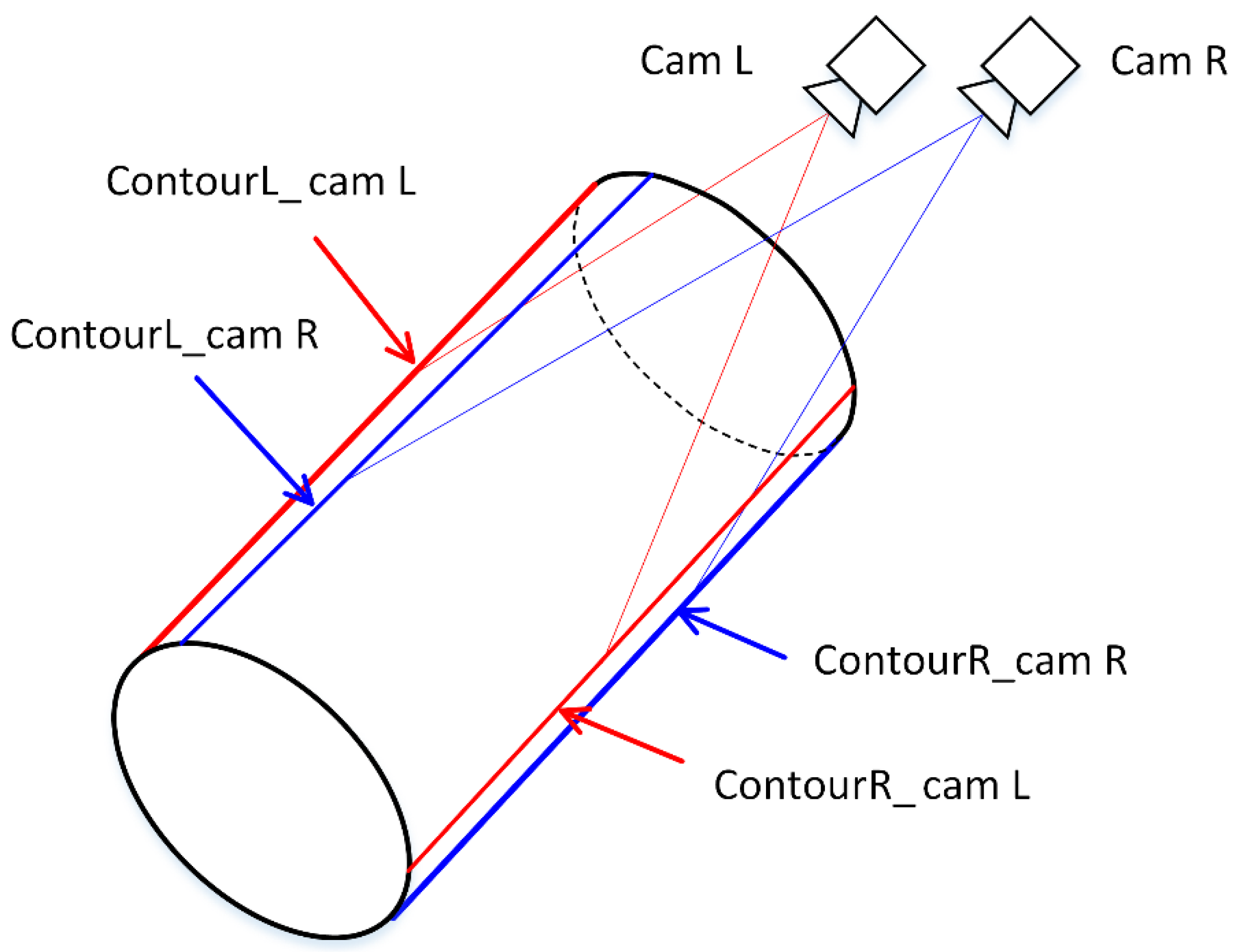
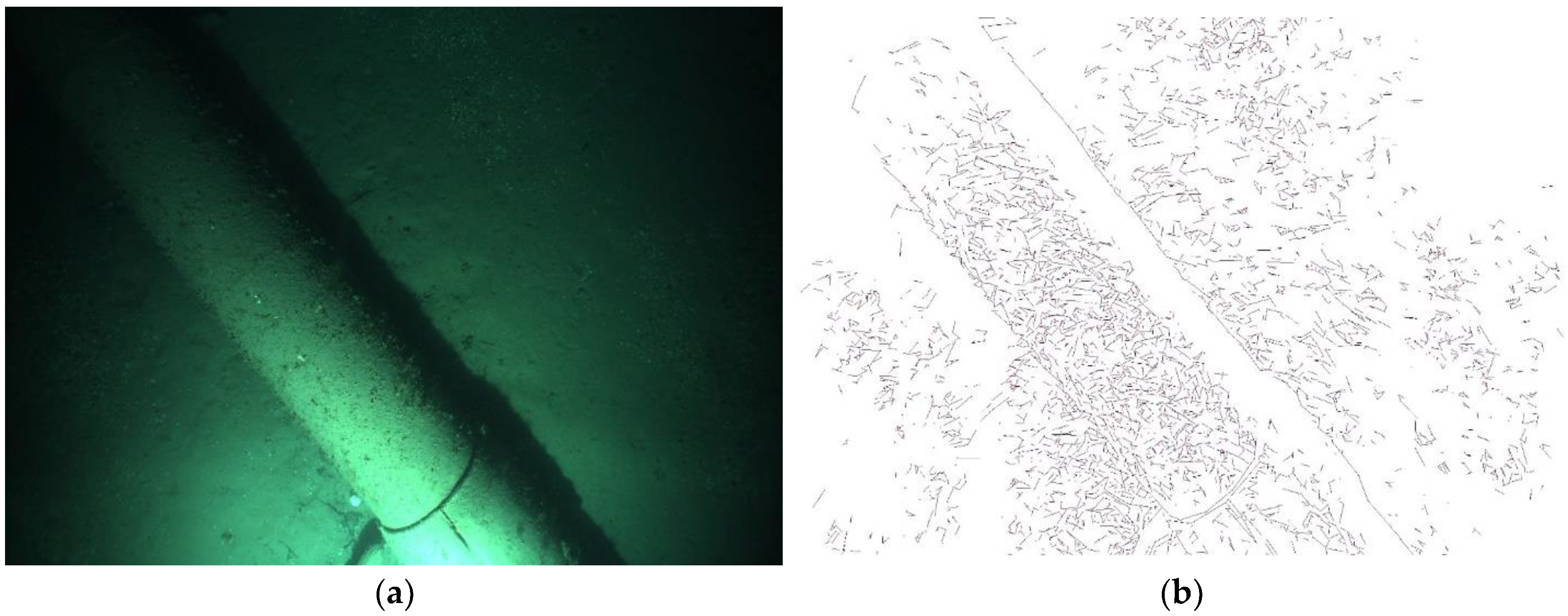
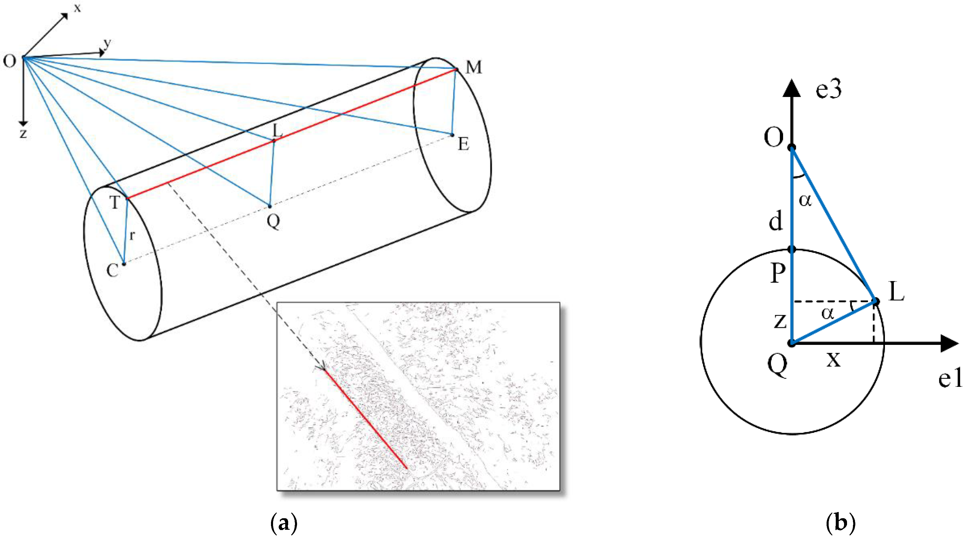
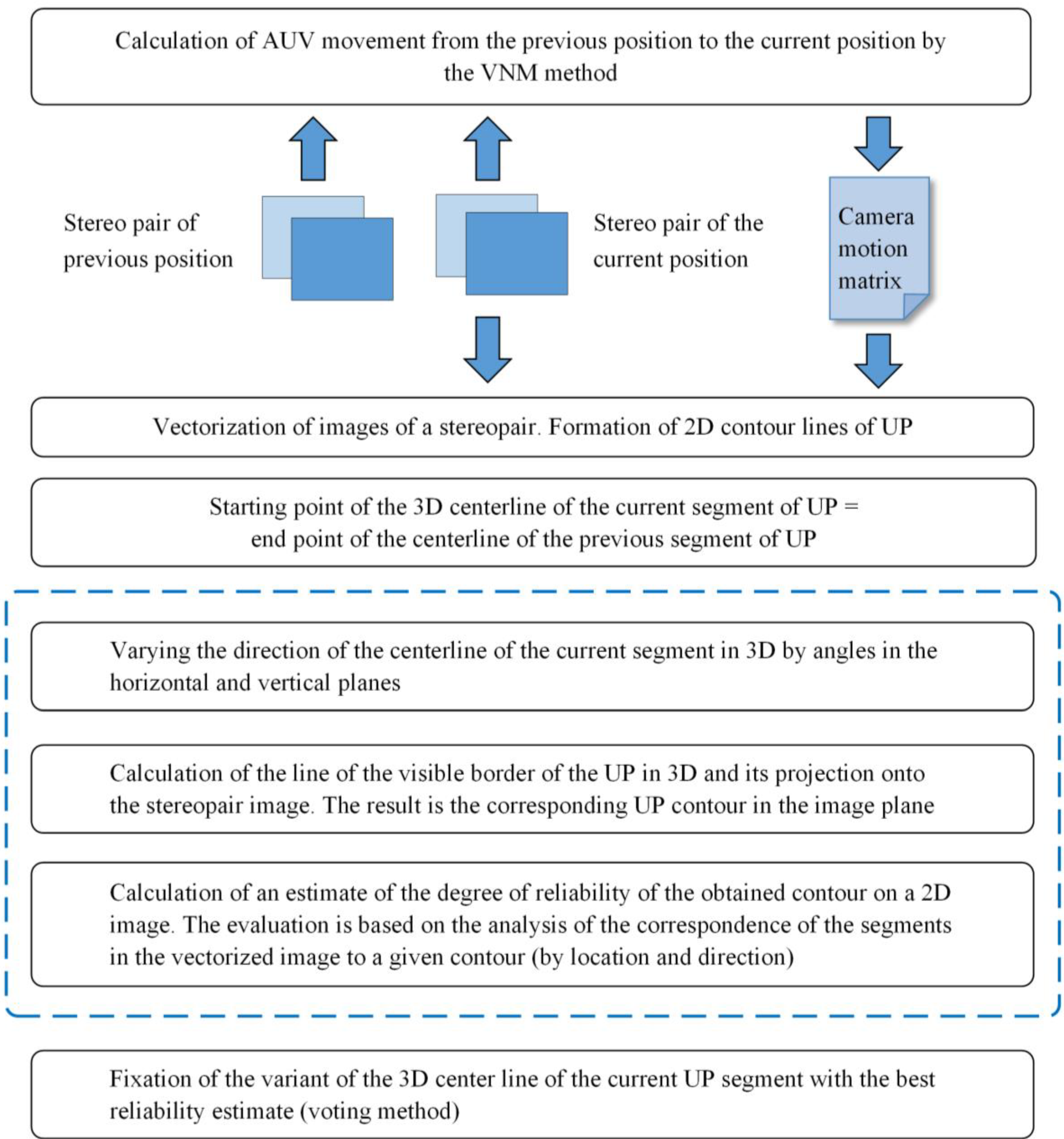
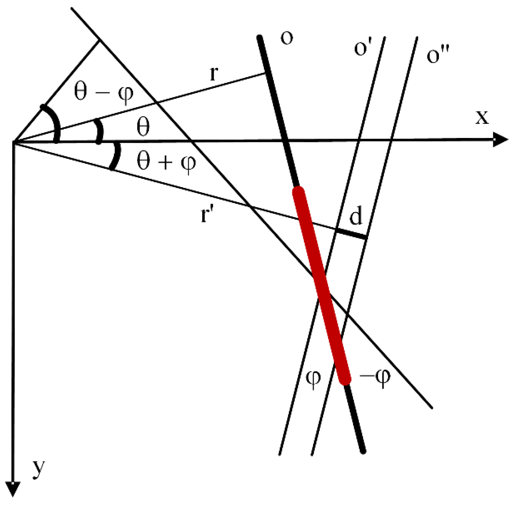


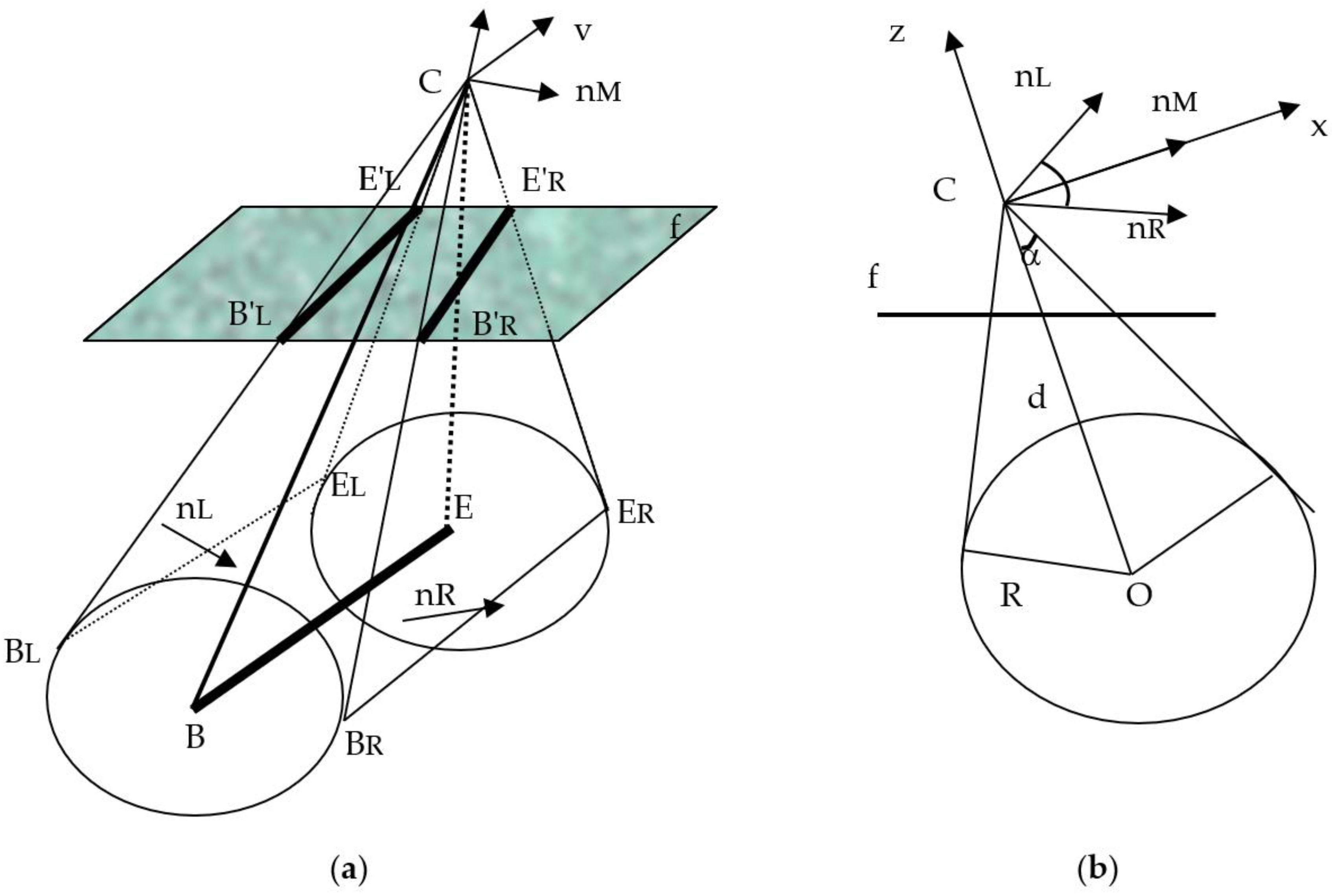
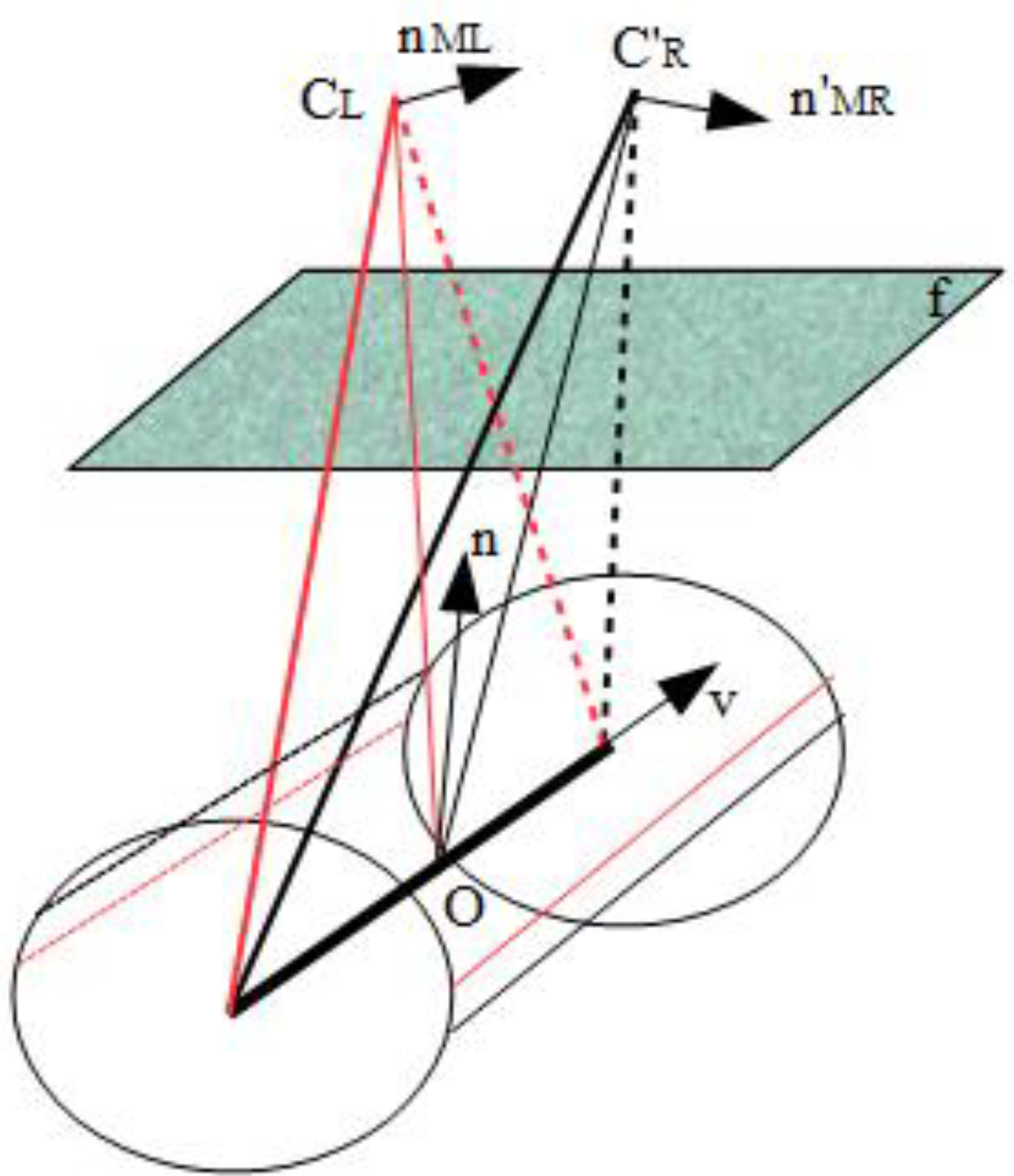

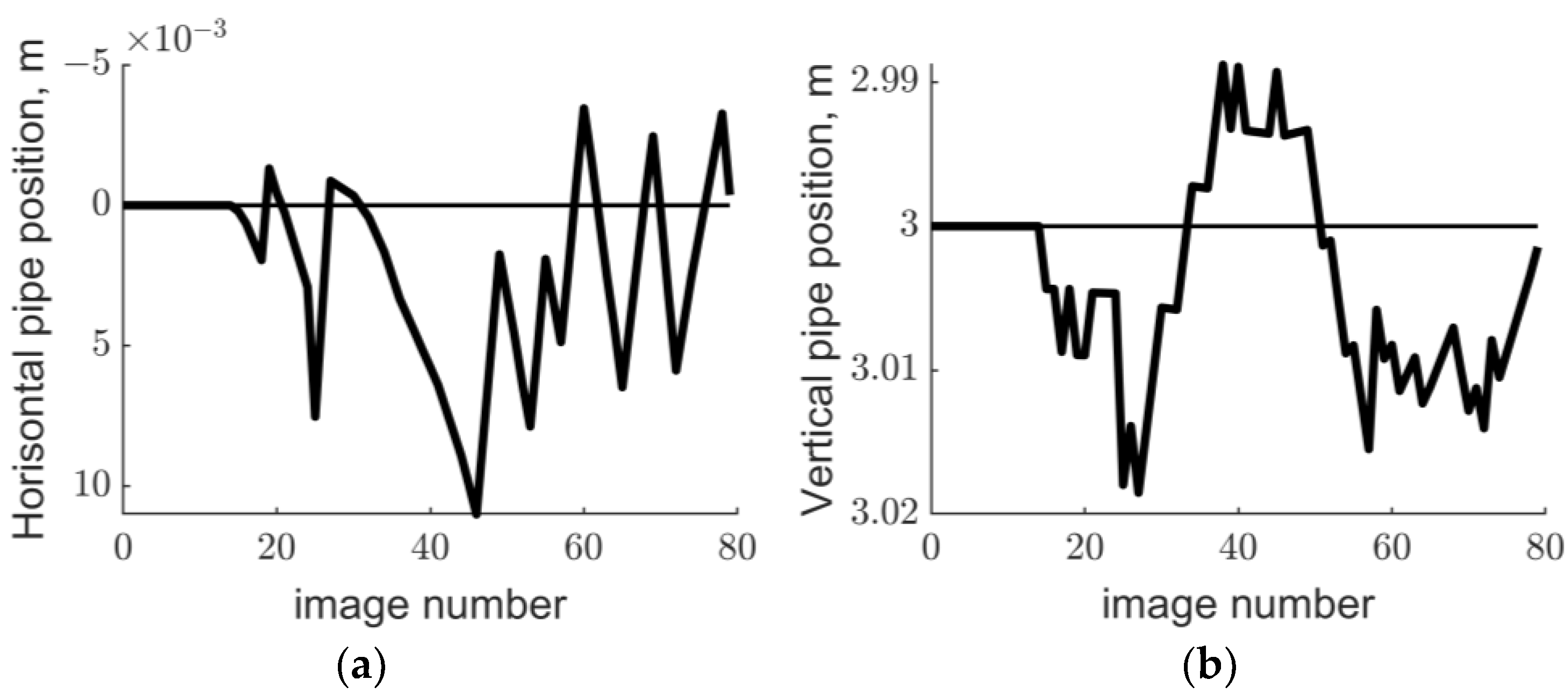
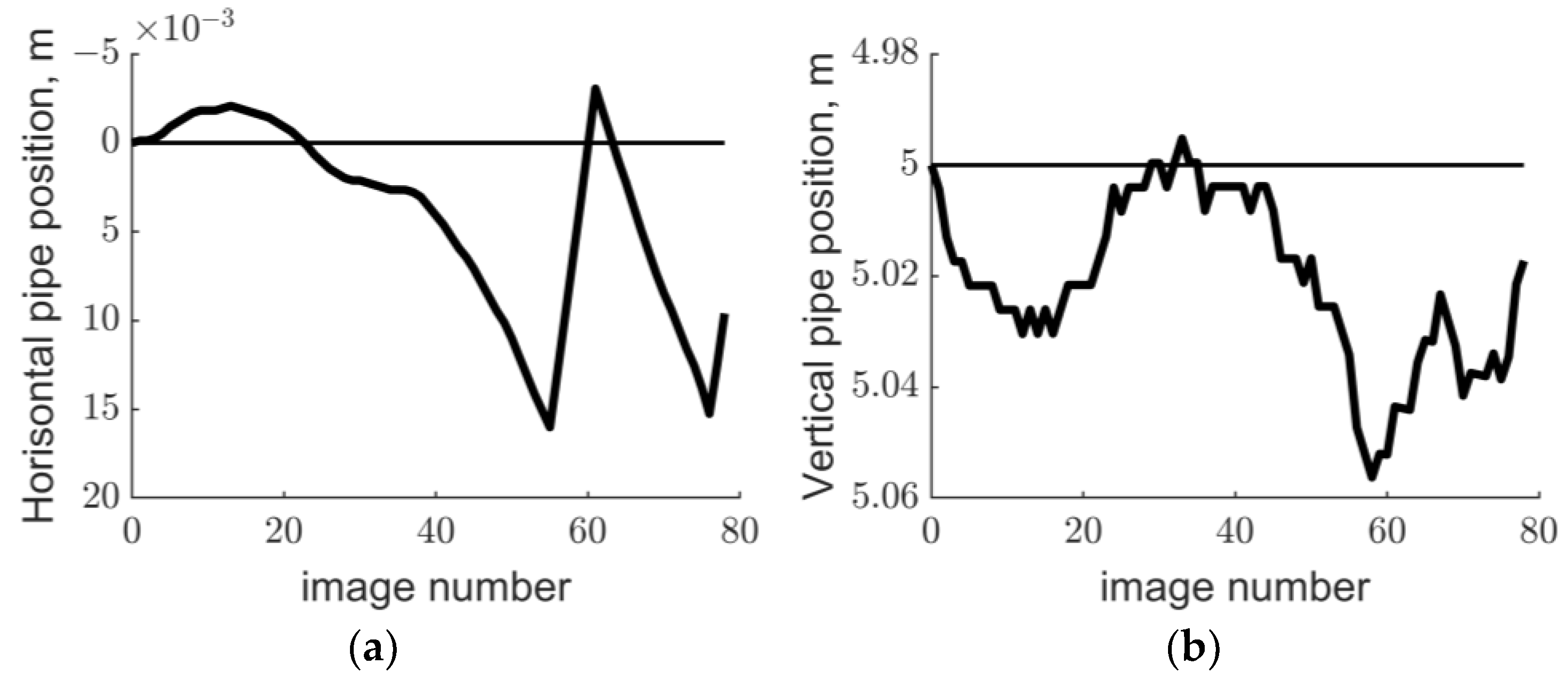
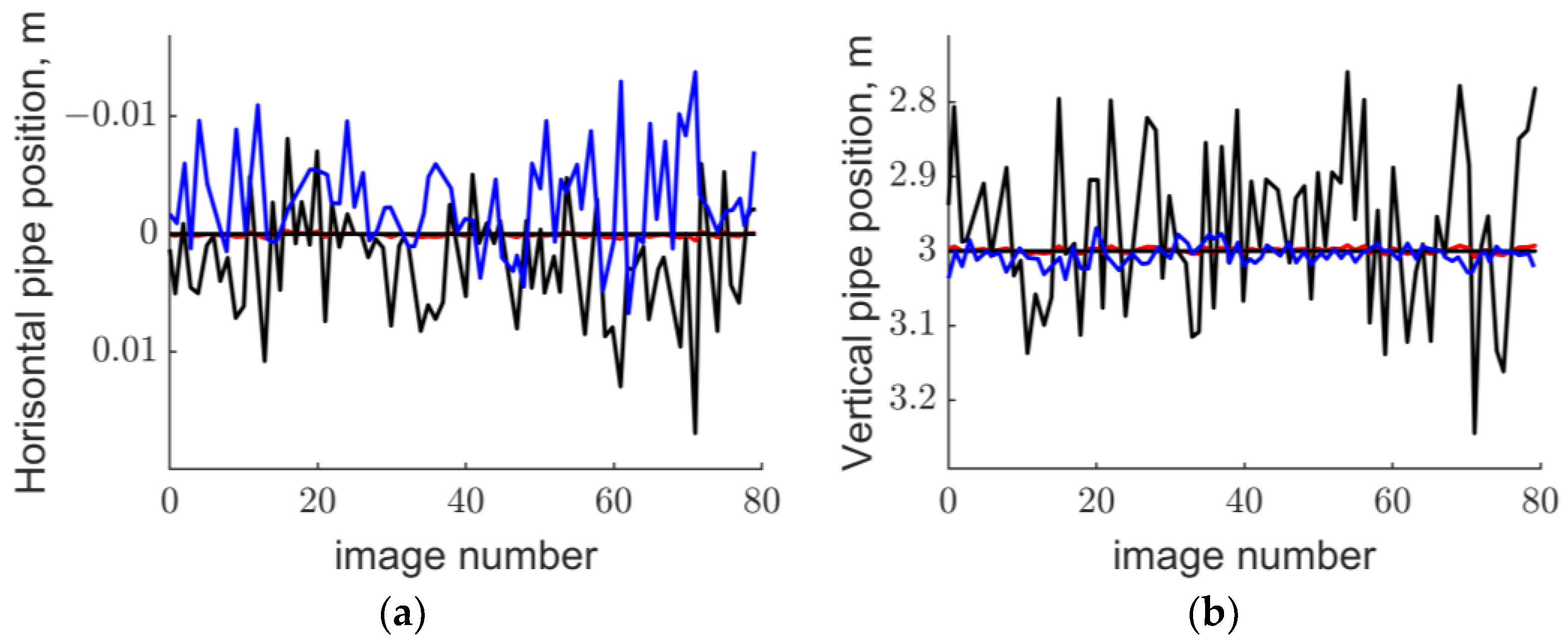


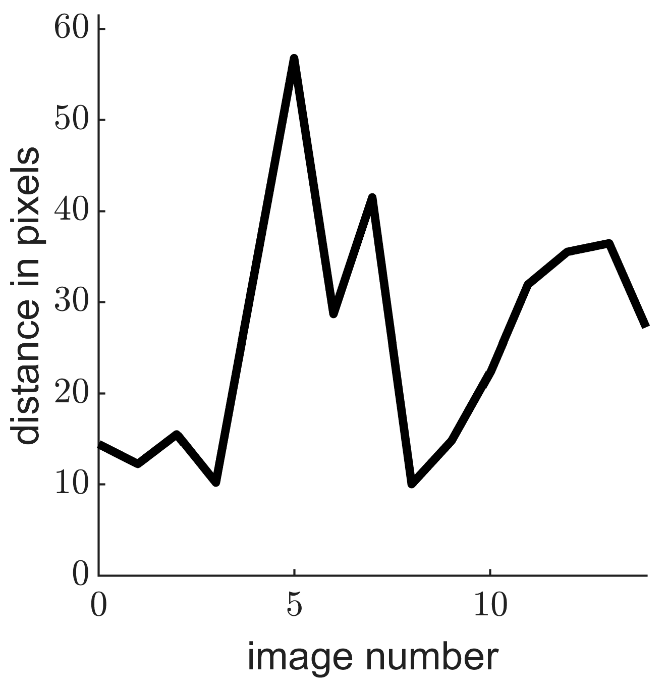
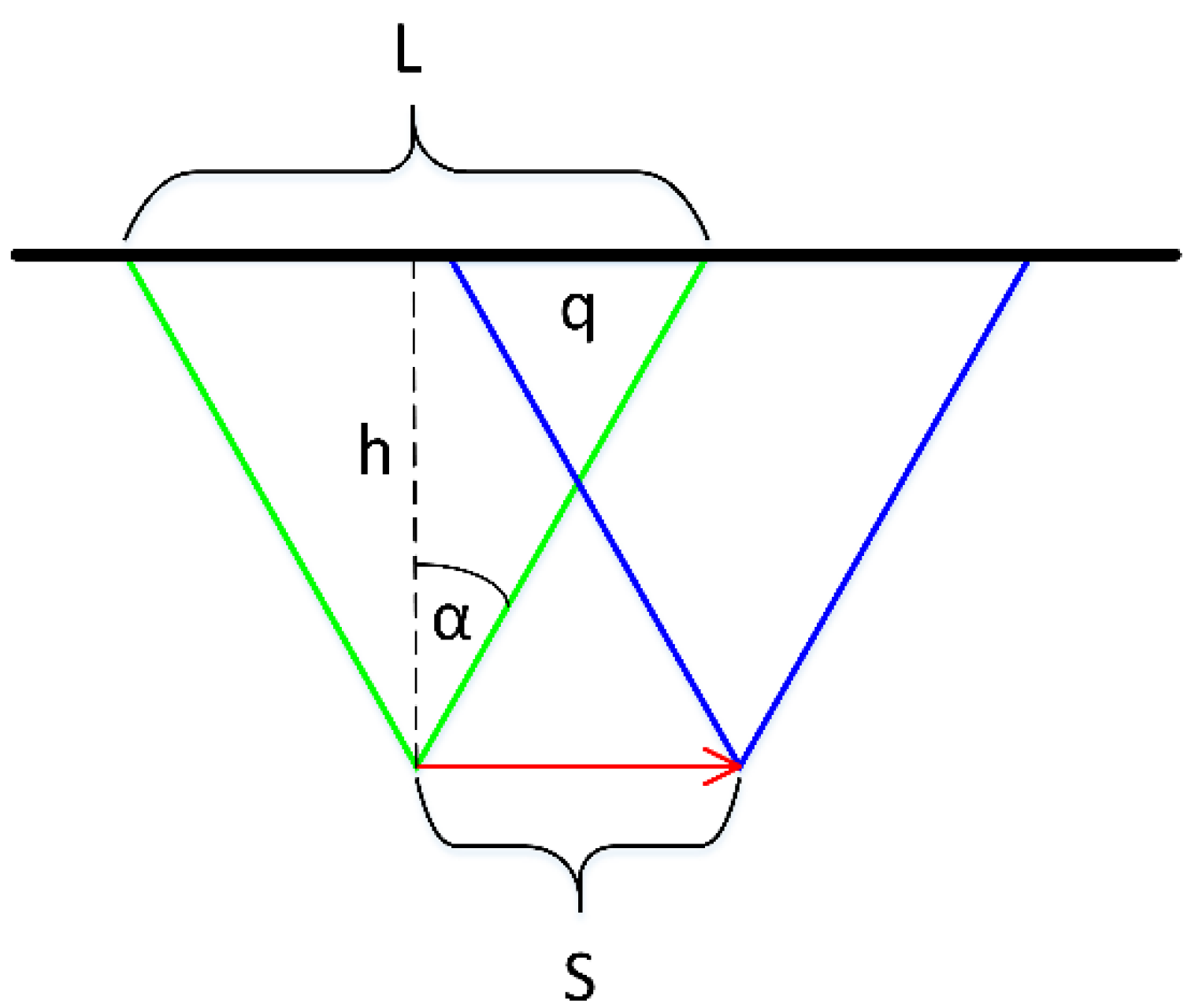
