Abstract
The growing sophistication of cyber threats necessitates robust and interpretable intrusion detection systems (IDS) to safeguard network security. While machine learning models such as Decision Tree (DT), Random Forest (RF), k-Nearest Neighbors (K-NN), and XGBoost demonstrate high effectiveness in detecting malicious activities, their interpretability decreases as their complexity and accuracy increase, posing challenges for critical cybersecurity applications. Local Interpretable Model-agnostic Explanations (LIME) is widely used to address this limitation; however, its reliance on normal distribution for perturbations often fails to capture the non-linear and imbalanced characteristics of datasets like CIC-IDS-2018. To address these challenges, we propose a modified LIME perturbation strategy using Weibull, Gamma, Beta, and Pareto distributions to better capture the characteristics of network traffic data. Our methodology improves the stability of different ML models trained on CIC-IDS datasets, enabling more meaningful and reliable explanations of model predictions. The proposed modifications allow for an increase in explanation fidelity by up to 78% compared to the default Gaussian approach. Pareto-based perturbations provide the best results. Among all distributions tested, Pareto consistently yielded the highest explanation fidelity and stability, particularly for K-NN ( = 0.9971, S = 0.9907) and DT ( = 0.9267, S = 0.9797). This indicates that heavy-tailed distributions fit well with real-world network traffic patterns, reducing the variance in attribute importance explanations and making them more robust.
1. Introduction
In today’s digital landscape, cyber threats are becoming increasingly sophisticated and pervasive, posing significant risks to the security and integrity of network infrastructures. From data breaches to advanced persistent threats, malicious actors continue to exploit vulnerabilities [1,2,3], making it imperative to develop robust intrusion detection systems (IDS) capable of identifying and mitigating such threats. Machine learning models such as k-Nearest Neighbor (kNN) [4,5,6], Decision Tree (DT) [7,8], Random Forest (RF) [9,10,11], and XGBoost have shown considerable promise in this domain due to their ability to analyze diverse network traffic patterns and detect malicious activities effectively [12]. These models offer varying strengths, from interpretability and simplicity in DT and RF to high performance and scalability in XGBoost [13,14]. However, despite their effectiveness, the black-box nature of deep networks poses a substantial challenge in terms of interpretability, particularly in critical applications like network security [15].
Local Interpretable Model-agnostic Explanations (LIME) is a widely used technique designed to explain the predictions of black-box models by creating locally interpretable models [16,17] around individual predictions. LIME generates these explanations by perturbing input data and analyzing the resulting model predictions. However, LIME’s assumption that the input data follows a normal distribution can lead to suboptimal and misleading explanations, especially when applied to datasets with non-normal distributions [18,19]. This issue becomes particularly relevant in the context of network intrusion detection, where datasets such as CIC-IDS-2017 and CIC-IDS-2018 are often highly imbalanced and exhibit non-normal distribution characteristics [20].
The CIC-IDS-2017 and CIC-IDS-2018 datasets, while widely adopted in the cybersecurity community, present a significant challenge due to the inherent imbalance in the distribution of network traffic classes. A small proportion of the dataset is malicious traffic, while the majority represents benign or normal traffic. This imbalance can skew learning in machine learning models, causing them to be biased toward the majority class and leading to poor performance in detecting underrepresented attack types. Traditional machine learning techniques often struggle to generalize effectively in such scenarios, facing reduced accuracy when dealing with minority classes.
Despite these advancements, interpretability remains a challenge. LIME has been widely adopted to address the black-box nature of machine and deep learning models by generating explanations based on input perturbations. However, the efficacy of LIME is greatly diminished when it encounters non-normally distributed data, which is common in network traffic datasets like CIC-IDS-2017 and CIC-IDS-2018. LIME operates assuming that the input data follows a normal distribution, leading it to generate perturbations that fail to capture the true distribution of network traffic. When LIME perturbs data points by introducing small changes based on normal distribution assumptions, it may create unrealistic data points that fall far outside the underlying distribution of the dataset. This can lead to explanations that are either inaccurate or uninformative, particularly when dealing with complex network traffic behaviors associated with various cyber-attacks.
In this paper, we address the limitations of LIME’s perturbation generation mechanism for non-normal distribution data by proposing a modified perturbation strategy. Our approach is tailored to handle the specific characteristics of imbalanced network traffic datasets, ensuring that the perturbations better reflect the actual distribution of the data. Through this, we enhance the quality of the explanations generated for machine learning models trained on CIC-IDS-2018, providing more accurate and meaningful insights into the detection of malicious network traffic. This modified methodology not only improves interpretability but also helps in validating and refining the decisions made by machine learning models, ultimately contributing to the development of more transparent and reliable intrusion detection systems.
2. Related Works
Explainable AI (XAI) methods, particularly for deep learning models like Transformers, often suffer from instability and inaccuracy due to the inherent complexity of these architectures [21]. Gradient-based approaches, while popular, focus only on local model behavior, failing to capture global dependencies that influence decisions. Attention mechanisms are frequently misinterpreted as explanations, even though their scores are shaped by scaling and softmax functions that distort their true importance. Layer Normalization (LayerNorm), a common component in Transformers, redistributes activations, which obscures the direct contributions of input features to model outputs. The lack of relevance conservation across layers in many XAI methods leads to the arbitrary attribution of importance, creating inconsistencies in explanations. Additionally, the sensitivity of certain models to small input perturbations amplifies noise, resulting in highly variable and unreliable relevance scores. Non-linear transformations within these models further complicate attribution, as traditional XAI techniques often fail to account for global context dependencies. Bias amplification is another concern, as XAI methods may inadvertently highlight spurious correlations or artifacts, misleading users. These shortcomings make explanations unreliable and prone to misinterpretation, particularly in sensitive applications.
Recent research highlights widely used explanation methods for AI models and their drastic inconsistencies across small input perturbations in certain circumstances [21]. Analyses demonstrate that commonly adopted local explanation techniques can produce contradictory outputs, raising concerns about reliability. Additionally, these methods often fail to capture the true reasoning behind model predictions, thereby creating a risk of misinterpretation. This shortcoming is further exacerbated by confounding factors that are challenging to isolate. Moreover, attention mechanisms used in XAI are frequently misinterpreted as explanations, even though their scores are shaped by scaling and softmax functions that distort their true importance. As a result, trust in the interpretability of complex models is undermined, particularly in high-stakes applications. Standard evaluation metrics do not fully account for explanation instability, thus offering a limited view of XAI effectiveness. The need for improved metrics and rigorous protocols to ensure that explanations align faithfully with underlying model behavior is often emphasized. Furthermore, a dual focus on both local and global interpretability is recommended. Ultimately, without rigorous validation, these explanation methods can create more confusion than clarity, highlighting the critical need for stability in XAI.
LIME—one of the XAI methodologies—is sensible to adversarial manipulation, exploiting its reliance on local perturbations to generate misleading explanations. Studies have shown how small, targeted changes in the input can cause drastic shifts in LIME’s feature importance attributions, highlighting a lack of robustness [22]. By strategically selecting or synthesizing perturbations that deviate from the original data distribution, it becomes possible to deceive LIME into allocating significance to irrelevant features. These manipulations underscore the fundamental limitations of LIME’s local linear approximation, which fails to capture the intricate global behavior of complex models. Additionally, LIME’s perturbation scheme often introduces synthetic examples that bear little resemblance to real data, thereby undermining the reliability of its explanations. This mismatch can lead to incorrect conclusions about which factors truly drive a model’s predictions. Another concern raised is LIME’s dependence on kernel-based weighting, making its results highly sensitive to parameter settings. Subtle tweaks to sampling methods, neighborhood sizes, or kernel widths can create considerable variations in output explanations, revealing instability. Consequently, these flaws pose a serious challenge to the method’s credibility and suitability in domains where interpretability carries high stakes.
As these insufficiencies are widely known in the XAI communities, many different metrics are being proposed by the researchers to evaluate the quality of XAI explanations [21]. Fidelity is highlighted as a crucial metric, gauging how accurately an explanation reflects the true reasoning behind a model’s predictions. Completeness is another essential measure, focusing on whether all decisive factors guiding the model are captured within the explanation. Stability promotes the notion that minor changes in input should not trigger drastically different or inconsistent explanations. Monotonicity underscores that strengthened evidence for a specific outcome should align with a correspondingly intensified emphasis in the explanation. Continuity encourages explanations to adapt gradually in response to gradual variations in input. Faithfulness is introduced as a way to verify whether an explanation approach accurately depicts the model’s inner operations. Comprehensibility focuses on the clarity and ease with which human decision makers can interpret the explanation. Utility is emphasized to determine whether an explanation genuinely supports users in their objectives. Trust examines the degree of confidence users place in the model after receiving the explanation. Finally, plausibility evaluates how logically and intuitively the explanation aligns with domain-specific or common-sense standards.
Furthermore, scientific reasoning principles are being integrated into XAI systems to enhance clarity and reliability [23]. Formalized explanatory patterns are being developed, which incorporate domain-specific axioms and hypotheses, ensuring more consistent and verifiable explanations are derived. To evaluate these explanations, new metrics are being designed to gauge logical soundness, interpretability, and applicability. Some investigators are leveraging qualitative analyses to capture nuanced human insights, while others rely on quantitative techniques to systematically measure explanatory fidelity. New frameworks are emerging to help bridge the gap between theoretical explanations and real-world contexts through the continuous refinement of model parameters. Interdisciplinary collaborations are increasingly common, enabling experts from diverse fields to contribute to the establishment of robust validation criteria and foster more holistic explanatory models. Various prototype systems are being tested to automatically generate explanations that follow established scientific patterns and logically cohere with the relevant data. There is also a focus on ensuring that explanations align with ethical guidelines, particularly when decisions have critical societal implications. In parallel, ongoing research seeks to integrate user feedback into XAI design, refining explanatory outputs for different stakeholder needs. Ultimately, these concerted efforts aim to establish comprehensive, scientifically grounded methodologies that produce more trustworthy and transparent explanations.
Perturbation is a key technique used in XAI, providing insights into how subtle input variations impact model behavior. Recent studies demonstrate that systematically modifying data inputs can reveal vulnerabilities and biases, prompting developers to refine architectures for improved robustness [24]. Perturbation-based methods, such as those explored in local interpretability frameworks, have been shown to highlight critical decision boundaries and feature dependencies in high-dimensional spaces [25]. By strategically altering inputs, researchers can identify core explanatory factors, enhancing both transparency and confidence in deep learning systems [26]. Techniques involving structured noise infusion and domain-specific perturbations further aid in identifying brittle regions of a model’s decision surface [27]. These approaches underscore the interplay between feature importance and model fidelity, allowing stakeholders to validate that predictions are grounded in meaningful evidence. Moreover, experiments with generative perturbation mechanisms can pinpoint latent interactions among features, thereby facilitating more targeted model corrections. Researchers are also exploring hybrid strategies that combine local perturbations with global analysis, ensuring that explanations remain both context-aware and comprehensive. The ability to adapt perturbation methods to different data modalities ensures versatility across a range of applications, from image classification to natural language processing. Ultimately, these perturbation-centric techniques serve as a powerful lens through which to scrutinize, diagnose, and improve complex machine learning models, paving the way for more trustworthy and interpretable AI solutions.
The stability of explanations is a critical metric in evaluating their robustness and reliability, particularly in the context of network intrusion detection. Several studies have explored this aspect, focusing on how perturbation-based or surrogate model methods perform in the face of non-linear and imbalanced datasets, such as CIC-IDS-2017 and CIC-IDS-2018.
Table 1 provides an overview and comparison of these works, with a particular emphasis on stability values. Recent studies have examined the stability of explanation methods like LIME in machine learning for intrusion detection. Stability is typically measured using metrics such as Jaccard similarity or other feature consistency measures across multiple explanation runs. These works, provided in Table 1 aim to address the challenge of low stability caused by data imbalance, complex decision boundaries, and unrealistic perturbations.

Table 1.
Modified LIME stability results.
3. Dataset
The CIC-IDS2017 and CSE-CIC-IDS-2018 datasets are widely used in Intrusion Detection System (IDS) research due to their comprehensive network security insights. CIC-IDS2017 was created from five days of real network traffic data recorded from 3 July to 7 July 2017, with each record containing 79 attributes, including a label for one of 15 possible traffic classifications. This dataset covers various attack types, such as denial of service and brute force attacks, making it valuable for training IDS models.
The CSE-CIC-IDS-2018 dataset expands upon CIC-IDS-2017, significantly increasing the data volume with over 16 million network flows compared to the original’s 2.8 million [32]. It includes all original attack types, plus new web application threats like SQL injection, cross-site scripting (XSS), and command injection, which exploit vulnerabilities at the application layer [33]. These additions reflect modern attack trends, where web applications are frequent targets.
However, the CSE-CIC-IDS-2018 dataset still exhibits a significant class imbalance, with 82.66% of records belonging to the dominant class. To address this, merging the two datasets could increase the representation of underrepresented classes, enhancing the training of machine learning models [34]. Additionally, filtering out rare or outlier classes could help create a more balanced [35] and noise-free dataset, improving IDS performance. These datasets provide a solid foundation for advancing IDS research, allowing for the development of models that detect a wider range of traditional and modern attack vectors effectively. Finally, our dataset contained 28 classes. After feature filtering, 32 features were retained as follows: 7 categorical binary features (frequency skewed) and 25 numerical features.
LIME works by approximating the complex model locally around the prediction with a simpler, interpretable model—typically a linear model. However, this approach assumes that the model’s behavior is approximately linear in the local vicinity of the data point being explained. As for the inherently non-linear CIC-IDS datasets, this assumption does not hold because of the following reasons:
- Non-linear decision boundaries [36]: The actual decision boundaries of models trained on these datasets are highly non-linear. A linear surrogate model cannot accurately approximate these boundaries, even locally, leading to misleading explanations.
- Poor local approximation [37]: The non-linear interactions between features mean that small changes in the input can lead to significant changes in the output. LIME’s linear approximations fail to capture these sensitivities, resulting in explanations that do not reflect the true behavior of the model.
- Synthetic data generation issues [38]: LIME generates synthetic data around the instance to fit the local surrogate model. In high-dimensional, non-linear spaces, this synthetic data may not be representative of the actual data distribution, causing the surrogate model to be an inaccurate reflection of the model’s local behavior.
4. Materials and Methods
One of the key limitations of LIME is its reliance on the assumption that data follow a normal distribution when generating perturbations. LIME operates by perturbing input features and then building a locally interpretable model (often a linear model) around the prediction to explain the decision made by a black-box model. However, this assumption of normally distributed data can be problematic, particularly when applied to real-world datasets like CIC-IDS-2017 and CIC-IDS-2018, which exhibit non-normal distributions due to the inherent imbalance and diverse nature of network traffic [39].
When LIME perturbs features based on normal distribution assumptions, the generated data points may fall outside the range or structure of the actual data distribution. For instance, network traffic features such as packet size, protocol type, and duration often follow non-normal distributions and may be heavily skewed. As a result, LIME’s perturbations can generate unrealistic or irrelevant instances that are not representative of real-world network behavior. This distorts the locally interpretable model and leads to explanations that are misleading or inaccurate.
LIME prediction generation starts by sampling new data points in the vicinity of the instance being explained, generating a local dataset around it. The black-box model is then queried for predictions on these newly generated samples. Each sampled data point is assigned a proximity-based weight that reflects how close it is to the original instance. With these weighted samples and the corresponding predictions, LIME trains an interpretable model, a ridge regression, that captures the local behavior of the complex model. By examining the learned coefficients of the interpretable model, one can identify the most influential features in the prediction. LIME is model-agnostic, meaning it can be applied to any black-box model or learning algorithm without modification. This flexibility allows practitioners to gain insights into the predictive mechanisms of otherwise opaque models.
This section discusses the enhancements made to the LIME algorithm to address challenges in generating explanations for non-linear datasets and models. The adjustments emphasize the incorporation of dataset-specific characteristics, including the approach to sampling random data points by utilizing Beta [40], Gamma [41], Pareto [42], and Weibull [43,44] distributions, instead of the traditional Gaussian distribution, aiming to improve the robustness and relevance of the generated explanations.
4.1. Explanation Stability Evaluation
To assess the stability of explanations for a given label , we employ the following methodology:
- For label , we generate independent explanations by running the explanation model times. Each explanation produces a list of the top features, where is the set of the top features from the -th independent run, and is the total number of runs conducted for stability assessment.
- Pairwise Jaccard similarity calculation. For each unique pair of feature lists (, ) with , we calculate the Jaccard similarity , defined as follows:where denotes the number of features common to both explanations and is the total number of unique features across the pair. This similarity score quantifies the overlap between feature lists, capturing the consistency of feature selection between pairs of explanations.
- Mean similarity calculation for stability . We define the stability score as the mean of all pairwise Jaccard similarities, which reflects the overall consistency of feature selection across runs as follows:where is the stability score for label , ranging from 0 (indicating no stability) to 1 (indicating perfect stability across runs), and is the normalization factor that ensures the mean is computed across all unique pairs of explanations.
4.2. Explanation Fidelity Evaluation
To ensure quality while enhancing stability, we evaluate the fidelity of local explanations to see how well the surrogate model approximates the original complex model we are explaining. Although the original task might be classification, LIME fits a local linear model (ridge regression) to approximate the complex model’s predicted class probabilities, treating them as continuous values. Therefore, the score is used as a measure of fidelity as follows:
where
- —fidelity score for class;
- —number of data points (perturbed sample count);
- —original model’s prediction for data point (class probability);
- —surrogate model’s prediction for data point (fitted regression for class probability output);
- —mean of the original model’s predictions for the class.
4.3. Distributions
After analyzing the data, we observed that many attributes contain outliers. Therefore, it was necessary to remove 5% of the extreme values to improve the quality and reliability of the data analysis. Upon working with the processed data, it was noticed that the distributions are zero-inflated. Non-zero values for numerical features often appear right-skewed (similar to Pareto), indicating a possible log-normal, exponential, or other heavy-tailed distribution (see Figure 1). For example, attributes such as “Active Max” and “Active Min” follow zero-inflated distributions, with the value 0.0 dominating; however after removing the zero values, the remaining data are likely to follow a skewed distribution, which is possibly logarithmic or exponential (Figure 1a,b). The “BwD IAT Mean” distribution is heavily right-skewed, with a high concentration at 0.0 and very few values distributed across higher intervals (Figure 1c). This is consistent with a zero-inflated exponential or power-law-like distribution. The attributes with integer values and with lower cardinality, such as the “Destination Port”, have a distribution with a few dominant values and create a categorical-like distribution with sharp peaks at specific values (Figure 1d). There are also scattered frequencies across less-used port numbers, indicating that specific modes dominate the distribution. For the distribution of “Bwd Packets/s”, after removing 5% of the extremes, the data are zero-inflated, meaning that many flows have no backward packets per second. The non-zero values form a bell-shaped distribution, peaking at around 10,000 and resembling a Gaussian distribution (Figure 1e). The “Packet Length Variance” distribution has a bell-shaped, slightly right-skewed pattern for non-zero data. The non-zero portion could resemble a normal-like distribution, with most data concentrated around 110,000 and with a long tail for higher variances (Figure 1f). These two attributes are the only ones with distributions that resemble a Gaussian distribution.
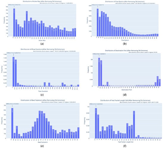
Figure 1.
Examples of distribution of selected attributes: (a) Active Max, (b) Flow Bytes(s), (c) BwD IAT Mean, (d) Destination Port, (e) Bwd Packets/s, (f) Packet Length Variance.
There are no normally distributed data in this dataset. Therefore, to approximate this distributional shape in the perturbations used by LIME, we employ parametric distributions such as Gamma, Beta, Pareto, and Weibull. These distributions are mathematically suitable for modeling heavy-tailored behaviors.
We selected heavy-tailed (Pareto), boundary-focused (Beta), skewed (Weibull/Gamma), and symmetrical (Gaussian) distributions to systematically explore different perturbations in LIME. By varying parameters (e.g., Pareto’s α from to , Weibull’s from to ), we capture incremental changes in tail weight or skewness at a consistent scale (). These choices highlight how LIME’s local explanations respond to domain-relevant noise shapes, testing robustness in extreme and boundary values.
The attribute values in this dataset exhibit a high concentration near zero, characterized by skewed tails extending asymmetrically away from zero, with minimal return probability. To approximate this distributional shape in the perturbations used by LIME, we employ parametric distributions such as Gamma, Beta, Pareto, and Weibull. These distributions are mathematically suitable for modeling heavy-tailored behaviors.
Gamma PDF (probability density function):
where is the shape parameter and is the scale parameter of the gamma distribution.
Beta PDF:
where are shape parameters.
Pareto PDF:
where is the shape parameter and is the scale parameter.
Weibull PDF:
where is the shape parameter and is the scale parameter.
4.4. Experimental Design
The experimental variables are provided in Table 2. The experiment constants include the use of ridge regression as the surrogate model for LIME, the generation of 5000 perturbed samples for each explanation, the consideration of the top 10 features for evaluation, and 30 explanation runs for each setup.
Table 2.
Experiment variables.
For each combination of test instance (3 labels), classification model (4 types), and distribution sampling method and parameters (13 configurations), explanations were generated and analyzed over 30 independent runs. Then, each set of explanations was evaluated by calculating the fidelity () and stability () metrics.
5. Results
5.1. Classification and Model Training
The performance of the three models, Decision Tree (DT), Random Forest (RF) and K-Nearest Neighbor (K-NN), was evaluated using confusion matrices to identify strengths and weaknesses in the classification of the different types of attacks (see Figure 2). It has been observed that DT performs the weakest due to its simplicity, struggling with complex decision boundaries, overlapping features (e.g., Web attacks, DDoS variants), and rare classes like “Heartbleed”. RF outperforms DT, with better generalization due to its ensemble nature, but it still faces challenges with class imbalances and rare attacks. K-NN performs well for well-separated classes but shows higher confusion in overlapping or imbalanced classes (e.g., “DoS” and “Brute Force” variants).
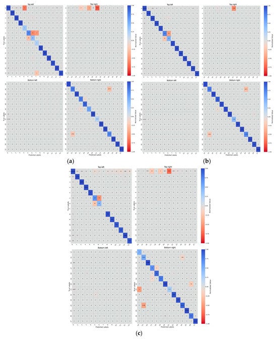
Figure 2.
Confusion matrix quadrants for the DT (a), RF (b), and K-NN (c) models with label mapping: {“BENIGN” (0), “DDoS” (1), “PortScan” (2), “Bot” (3), “Infiltration” (4), “Web Attack Brute Force” (5), “Web Attack XSS” (6), “Web Attack SQL Injection” (7), “FTP-Patator” (8), “SSH-Patator” (9), “DoS Slowloris” (10), “DoS Slowhttptest” (11), “DoS Hulk” (12), “DoS GoldenEye” (13), “Heartbleed” (14), “DoS Attacks-SlowHTTPTest” (15), “DoS Attacks-Hulk” (16), “Brute Force-Web” (17), “Brute Force-XSS” (18), “SQL Injection” (19), “DDoS Attacks-LOIC-HTTP” (20), “Infilteration” (21), “DoS Attacks-GoldenEye” (22), “DoS Attacks-Slowloris” (23), “FTP-BruteForce” (24), “SSH-Bruteforce” (25), “DDoS Attack-LOIC-UDP” (26), “DDoS Attack-HOIC” (27)}.
The “BENIGN” class is generally the easiest to identify across all models due to its distinct characteristics and dominance in most datasets. However, some confusion may still arise, with occasional misclassification of “BENIGN” as attack classes like “Bot” (3), “DDoS” (1), and “Infilteration” (21).
All three models show significant confusion among web attack classes, such as “Web Attack Brute Force” (5) and “Web Attack XSS” (6). Classes like “DoS Slowloris” (10), “DoS Slowhttptest” (11), “DoS Attacks-SlowHTTPTest” (15), and “DoS Attacks-Hulk” (16) are frequently confused across all models, especially in K-NN. Overlapping traffic patterns and attack methodologies explain these confusions. Rare classes, such as “Infiltration” (4) and “Heartbleed” (14), are often misclassified into other classes, especially in DT, due to insufficient training data.
The model training results, provided in Table 3, demonstrate high performance across all metrics. To ensure consistency and robustness, 5-fold cross-validation was applied to all models. XGBoost (XGB), trained with , and , achieved the highest weighted accuracy (0.9995) and strong macro-level metrics (, ). The RF method using and , followed closely, with a weighted accuracy of 0.99875. DT () and k-Nearest Neighbor (kNN) () also performed well but showed slightly lower macro-level metrics. The best results for CATBoost (CATB) were obtained with , the default regularization value of , and with chosen as the method for sampling the data and subsample ().
Table 3.
Classification model training results.
5.2. Explanation Fidelity
The performance of the different feature perturbation distributions in the LIME framework reflects the fidelity of its explanations. This fidelity is quantified by the average score, which measures how well the LIME surrogate model approximates the decision boundaries of the underlying black-box models. A higher value indicates better fidelity, as it reflects a closer match between the surrogate model and the original model.
Table 4 summarizes the average explanation fidelity () for surrogate models generated by LIME using various sampling distributions.
Table 4.
Average explanation fidelity (R2) across models and sampling distributions.
The results demonstrate that all selected distributions (Pareto, Weibull, Beta, and Gamma) significantly outperform the default Gaussian distribution in capturing the decision boundaries of the base classifiers. Pareto () achieves the highest for the Decision Tree (0.9267) and kNN (0.9971), while Weibull () achieves the best fidelity for XGB (0.6042). However, the fidelity scores decrease as the model complexity increases, with XGB and Random Forest showing consistently lower values across all distributions, highlighting the challenges LIME faces in approximating complex decision boundaries. These findings emphasize that using perturbation distributions, aligned with the data, significantly enhances explanation fidelity, particularly for simpler models like Decision Tree and kNN. Figure 3 aggregates scores for Weibull and Pareto distributions and illustrates how the average fidelity varies across models.
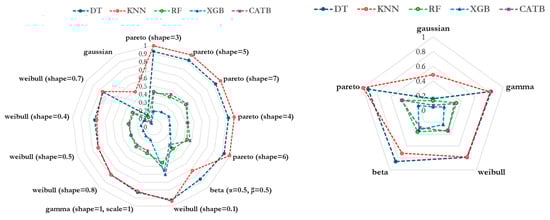
Figure 3.
Average explanation fidelity () across models and sampling distributions. Left: R2 scores for individual distribution parameterizations. Right: Averaged R2 scores for each distribution family.
5.3. Explanation Stability
The stability of explanations within the LIME framework is a critical metric for evaluating its robustness and consistency. Explanation stability is quantified by measuring how consistently the LIME-generated explanations align when subjected to minor perturbations in the input data or variations in the sampling process. A higher stability score indicates more reliable explanations, signifying that the model’s interpretation remains unaffected by slight changes, thereby fostering trust in its utility for decision-making.
Table 5 highlights the stability () of LIME-generated explanations across models and distributions, measured using the Jaccard similarity of the top 10 features. Pareto distributions consistently achieve the highest stability across models, particularly for simpler models like KNN () and Decision Tree (). Beta and Gamma distributions also perform significantly better than Gaussian distributions, with Beta showing strong stability for Decision Tree and Gamma performing well for Random Forest. Decision Tree shows the greatest variability in stability, ranging from (Gaussian) to (Pareto), reflecting its sensitivity to the choice of sampling distribution. In contrast, more complex models like XGB and RF show less variability across distributions, though their overall stability remains lower. CATB follows a similar pattern to XGB and RF, maintaining relatively stable explanation consistency across distributions but showing lower stability under Weibull and Gaussian sampling.
Table 5.
Average explanation stability () across models and sampling distributions.
By averaging across different parameter configurations for Pareto and Weibull distributions, Figure 4 demonstrates the overall superiority of Pareto in producing stable LIME on this dataset.
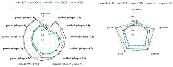
Figure 4.
Average explanation stability () across models and sampling distributions. Left: stability (S) scores for individual distribution parameterizations. Right: Averaged stability (S) scores for each distribution family.
The stability of explanations across runs for a Decision Tree model applied to a “Benign” class instance is shown in Figure 5. On the left, the bar charts illustrate the top 10 features and their explanation scores for the first and second runs of the same instance. In Subfigure (a) (Gaussian distribution), the fifth and sixth most influential features disappear between runs, indicating variability in feature importance rankings. In Subfigure (b) (Pareto distribution, shape = 3), the top 10 features remain unchanged across runs, showcasing higher stability. On the right, the Jaccard similarity matrix quantifies pairwise similarities across all 30 runs. The Gaussian distribution exhibits lower similarity scores, reflecting greater variability in explanations, while the Pareto distribution shows consistently high similarity scores, confirming the stability seen in the left-side bar charts.
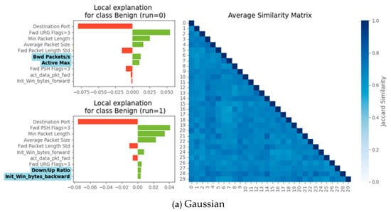
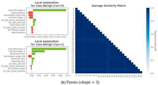
Figure 5.
Run-level explainability stability: Gaussian vs. non-Gaussian distributions. Left: Top 10 features and their explanation scores for the first and second explain runs of the same instance. Features highlighted in blue appear in one run but not the other. Right: JS matrix showing pairwise similarities across runs (n = 30). Subfigure (a) corresponds to the Gaussian distribution, and subfigure (b) to the Pareto distribution (shape = 3). The explained model is a DT, and the test data instance is from the “Benign” class.
5.4. Overall Evaluation of Sampling Distributions
Table 6 provides a comparison of sampling distributions based on their summed ranks for the average fidelity () and stability () of LIME across models. For our dataset, Pareto distributions consistently perform the best when considering both metrics. Pareto () has the lowest summed rank, indicating it achieves the best overall balance between fidelity and stability, closely followed by Pareto (). In contrast, Gaussian has the highest summed rank, ranking last in both fidelity and stability, reinforcing its limitations as the default perturbation distribution. These summed rank comparisons clearly demonstrate that Pareto distributions are the most effective for generating both stable and high-fidelity LIME on this dataset.
Table 6.
Averaged stability and fidelity of explanations across models.
6. Discussion
From our experiments, we found that it would be useful to investigate different disturbance methods for each attribute in future studies. This approach would allow for the development of disturbance strategies that are more relevant to the specific distributional and structural characteristics of individual attributes, thus increasing the robustness and interpretability of the LIME system when dealing with datasets that include a mix of continuous, categorical, and binary attributes, as they allow for more accurate representation of real-world data distributions during the perturbation process
Perturbation methods for categorical attributes should take into account the discrete and non-ordinary nature of such attributes. The random selection of categories according to their observed probabilities or by applying domain-specific rules could help maintain data integrity. To ensure that common categories are perturbed more frequently, frequency-weighted sampling can be applied. Techniques to generate more realistic category combinations and avoid invalid or nonsensical perturbations, etc., are recommended. Moreover, in datasets, we often have binary attributes, so perturbations can involve flipping the value (e.g., from 0 to 1 or vice versa) with a probability that reflects the distribution of the binary class in the dataset. In addition, it is reasonable to explore such techniques as class-conditional perturbations, noise injection in binary features, in order to examine the model’s sensitivity to minor and other changes.
7. Conclusions
This study addresses the critical challenges in the interpretability of machine learning models for intrusion detection, particularly when applied to complex, imbalanced datasets such as CIC-IDS-2018. While machine learning models such as k-Nearest Neighbors, Decision Trees, Random Forests, and XGB demonstrate strong performance in detecting malicious network traffic, the black-box nature of these models often limits their practical utility in cybersecurity applications, where interpretability and trust are paramount. Local Interpretable Model-agnostic Explanations (LIME), a commonly used explanation method, was evaluated for its limitations in handling datasets with non-normal distributions, which are common in real-world network traffic.
Through this research, a modified LIME framework was proposed, incorporating alternative perturbation sampling methods such as Pareto, Weibull, Beta, and Gamma distributions to better align with the underlying data characteristics. Experimental results demonstrate that these modifications significantly enhance both the fidelity and stability of explanations compared to the default Gaussian perturbation approach. Pareto distributions, in particular, achieved the best balance between fidelity and stability across various machine learning models, highlighting their suitability for high-dimensional, imbalanced datasets.
The evaluation metrics, including explanation fidelity (R2) and stability (S), showed marked improvements, especially for simpler models like Decision Trees and k-Nearest Neighbors. However, challenges remain in achieving similarly high levels of fidelity and stability for more complex models like XGB and Random Forests, which exhibit intricate, non-linear decision boundaries.
This research contributes to advancing the interpretability of intrusion detection systems by improving the quality of explanations generated for machine learning models. These enhancements not only aid in validating and refining model decisions but also foster trust in their deployment for cybersecurity applications. Future work will focus on further refining perturbation strategies and exploring hybrid explanation methods to extend interpretability to more complex models and dynamic network environments.
Author Contributions
Conceptualization, A.P.-T.; data curation: M.B. and A.P.-T.; investigation, M.B. and A.P.-T.; methodology, M.B. and A.P.-T.; software, M.B., A.P.-T., G.Z., L.K. and A.M.; resources M.B., A.P.-T., G.Z., L.K. and A.M.; validation M.B.; writing—original draft, M.B. and A.P.-T.; writing—review and editing, M.B., G.Z., L.K., A.M. and A.P.-T.; supervision, A.P.-T. All authors have read and agreed to the published version of the manuscript.
Funding
This research/project was co-funded by the European Union under Horizon Europe program grant agreement No. 101059903, the European Union funds for the period 2021–2027, and the state budget of the Republic of Lithuania financial agreement No. 10-042-P-0001.
Data Availability Statement
https://github.com/zokaityte/LIME-Explainability-Stability (accessed on 12 February 2025).
Conflicts of Interest
The authors declare no conflicts of interest.
References
- Ahmad, Z.; Shahid Khan, A.; Wai Shiang, C.; Abdullah, J.; Ahmad, F. Network intrusion detection system: A systematic study of machine learning and deep learning approaches. Trans. Emerg. Telecommun. Technol. 2021, 32, e4150. [Google Scholar] [CrossRef]
- Kumar, S.; Dwivedi, M.; Kumar, M.; Gill, S.S. A comprehensive review of vulnerabilities and AI-enabled defense against DDoS attacks for securing cloud services. Comput. Sci. Rev. 2024, 53, 100661. [Google Scholar] [CrossRef]
- Alanazi, M.; Mahmood, A.; Chowdhury, M.J.M. SCADA vulnerabilities and attacks: A review of the state-of-the-art and open issues. Comput. Secur. 2023, 125, 103028. [Google Scholar] [CrossRef]
- Guo, G.; Wang, H.; Bell, D.; Bi, Y.; Greer, K. KNN Model-Based Approach in Classification. In Proceedings of the on the Move to Meaningful Internet Systems 2003: CoopIS, DOA, and ODBASE, Catania, Italy, 3–7 November 2003; Meersman, R., Tari, Z., Schmidt, D.C., Eds.; Springer: Berlin/Heidelberg, Germany, 2003; pp. 986–996. [Google Scholar] [CrossRef]
- Li, W.; Yi, P.; Wu, Y.; Pan, L.; Li, J. A New Intrusion Detection System Based on KNN Classification Algorithm in Wireless Sensor Network. J. Electr. Comput. Eng. 2014, 2014, 240217. [Google Scholar] [CrossRef]
- Ding, H.; Chen, L.; Dong, L.; Fu, Z.; Cui, X. Imbalanced data classification: A KNN and generative adversarial networks-based hybrid approach for intrusion detection. Future Gener. Comput. Syst. 2022, 131, 240–254. [Google Scholar] [CrossRef]
- Thombre, A. Comparison of decision trees with Local Interpretable Model-Agnostic Explanations (LIME) technique and multi-linear regression for explaining support vector regression model in terms of root mean square error (RMSE) values. arXiv 2024, arXiv:2404.07046. [Google Scholar] [CrossRef]
- Priyanka; Kumar, D. Decision tree classifier: A detailed survey. Int. J. Inf. Decis. Sci. 2020, 12, 246–269. [Google Scholar] [CrossRef]
- Panda, M.; Mahanta, S.R. Explainable artificial intelligence for Healthcare applications using Random Forest Classifier with LIME and SHAP. arXiv 2023, arXiv:2311.05665. [Google Scholar] [CrossRef]
- Prabhu, H.; Sane, A.; Dhadwal, R.; Parlikkad, N.R.; Valadi, J.K. Interpretation of Drop Size Predictions from a Random Forest Model Using Local Interpretable Model-Agnostic Explanations (LIME) in a Rotating Disc Contactor. Ind. Eng. Chem. Res. 2023, 62, 19019–19034. [Google Scholar] [CrossRef]
- Shaik, A.B.; Srinivasan, S. A Brief Survey on Random Forest Ensembles in Classification Model. In Proceedings of the International Conference on Innovative Computing and Communications, Delhi, India, 5–6 May 2018; Bhattacharyya, S., Hassanien, A.E., Gupta, D., Khanna, A., Pan, I., Eds.; Springer: Singapore, 2018; pp. 253–260. [Google Scholar] [CrossRef]
- Pai, V.; Devidas; Adesh, N.D. Comparative analysis of Machine Learning algorithms for Intrusion Detection. IOP Conf. Ser. Mater. Sci. Eng. 2021, 1013, 012038. [Google Scholar] [CrossRef]
- Ribeiro, M.T.; Singh, S.; Guestrin, C. Model-Agnostic Interpretability of Machine Learning. arXiv 2016, arXiv:1606.05386. [Google Scholar] [CrossRef]
- Le, T.-T.-H.; Oktian, Y.E.; Kim, H. XGBoost for Imbalanced Multiclass Classification-Based Industrial Internet of Things Intrusion Detection Systems. Sustainability 2022, 14, 8707. [Google Scholar] [CrossRef]
- Neupane, S.; Ables, J.; Anderson, W.; Mittal, S.; Rahimi, S.; Banicescu, I.; Seale, M. Explainable Intrusion Detection Systems (X-IDS): A Survey of Current Methods, Challenges, and Opportunities. IEEE Access 2022, 10, 112392–112415. [Google Scholar] [CrossRef]
- Ribeiro, M.T.; Singh, S.; Guestrin, C. Anchors: High-Precision Model-Agnostic Explanations. Proc. AAAI Conf. Artif. Intell. 2018, 32, 1527–1535. [Google Scholar] [CrossRef]
- Lundberg, S.; Lee, S.-I. A Unified Approach to Interpreting Model Predictions. arXiv 2017, arXiv:1705.07874. [Google Scholar] [CrossRef]
- Molnar, C. Interpretable Machine Learning, 2nd ed.; Leanpub: Victoria, BC, Canada, 2018; Available online: https://leanpub.next/interpretable-machine-learning (accessed on 25 November 2024).
- Demšar, J. Statistical Comparisons of Classifiers over Multiple Data Sets. J. Mach. Learn. Res. 2006, 7, 1–30. [Google Scholar]
- Sharafaldin, I.; Habibi Lashkari, A.; Ghorbani, A.A. Toward Generating a New Intrusion Detection Dataset and Intrusion Traffic Characterization. In Proceedings of the 4th International Conference on Information Systems Security and Privacy (ICISSP 2018), Funchal, Portugal, 22–24 January 2018; SCITEPRESS—Science and Technology Publications: Setubal, Portugal, 2018; pp. 108–116. [Google Scholar] [CrossRef]
- Ali, A.; Schnake, T.; Eberle, O.; Montavon, G.; Müller, K.-R.; Wolf, L. XAI for Transformers: Better Explanations through Conservative Propagation. arXiv 2022, arXiv:2202.07304. [Google Scholar] [CrossRef]
- Wilking, R.; Jakobs, M.; Morik, K. Fooling Perturbation-Based Explainability Methods. Presented at the Workshop on Trustworthy Artificial Intelligence as a Part of the ECML/PKDD 22 Program, IRT SystemX [IRT SystemX], Grenoble, France, 19 September 2022; Available online: https://zendy.io/title/PROCART-668565028 (accessed on 8 January 2025).
- Zhao, H.; Chen, H.; Yang, F.; Liu, N.; Deng, H.; Cai, H.; Wang, S.; Yin, D.; Du, M. Explainability for Large Language Models: A Survey. arXiv 2023, arXiv:2309.01029. [Google Scholar] [CrossRef]
- Ivanovs, M.; Kadikis, R.; Ozols, K. Perturbation-based methods for explaining deep neural networks: A survey. Pattern Recognit. Lett. 2021, 150, 228–234. [Google Scholar] [CrossRef]
- Agarwal, S.; Jabbari, S.; Agarwal, C.; Upadhyay, S.; Wu, Z.S.; Lakkaraju, H. Towards the Unification and Robustness of Perturbation and Gradient Based Explanations. arXiv 2021, arXiv:2102.10618. [Google Scholar] [CrossRef]
- Robnik-Šikonja, M.; Bohanec, M. Perturbation-Based Explanations of Prediction Models. In Human and Machine Learning; Zhou, J., Chen, F., Eds.; Springer: Cham, Switzerland, 2024. [Google Scholar] [CrossRef]
- Jiang, E. UniformLIME: A Uniformly Perturbed Local Interpretable Model-Agnostic Explanations Approach for Aerodynamics. J. Phys. Conf. Ser. 2022, 2171, 012025. [Google Scholar] [CrossRef]
- Zhou, Z.; Hooker, G.; Wang, F. S-LIME: Stabilized-LIME for Model Explanation. In Proceedings of the 27th ACM SIGKDD Conference on Knowledge Discovery & Data Mining, Singapore, 14–18 August 2021; pp. 2429–2438. [Google Scholar] [CrossRef]
- Bora, R.P.; Terhorst, P.; Veldhuis, R.; Ramachandra, R.; Raja, K. SLICE: Stabilized LIME for Consistent Explanations for Image Classification. In Proceedings of the 2024 IEEE/CVF Conference on Computer Vision and Pattern Recognition (CVPR), Seattle, WA, USA, 16–22 June 2024. [Google Scholar]
- Meng, H.; Wagner, C.; Triguero, I. An Initial Step Towards Stable Explanations for Multivariate Time Series Classifiers with LIME. In Proceedings of the 2023 IEEE International Conference on Fuzzy Systems (FUZZ), Incheon, Republic of Korea, 13–17 August 2023; pp. 1–6. [Google Scholar] [CrossRef]
- Saadatfar, H.; Kiani-Zadegan, Z.; Ghahremani-Nezhad, B. US-LIME: Increasing fidelity in LIME using uncertainty sampling on tabular data. Neurocomputing 2024, 597, 127969. [Google Scholar] [CrossRef]
- Error Prevalence in NIDS Datasets: A Case Study on CIC-IDS-2017 and CSE-CIC-IDS-2018. IEEE Conference Publication. IEEE Xplore. Available online: https://ieeexplore.ieee.org/abstract/document/9947235 (accessed on 25 November 2024).
- Nair, S.S. Securing Against Advanced Cyber Threats: A Comprehensive Guide to Phishing, XSS, and SQL Injection Defense. J. Comput. Sci. Technol. Stud. 2024, 6, 76–93. [Google Scholar] [CrossRef]
- Han, J.; Pei, J.; Tong, H. Data Mining: Concepts and Techniques; Morgan Kaufmann: Burlington, MA, USA, 2022; ISBN 978-0-12-811761-3. [Google Scholar]
- Silva, J.V.V.; de Oliveira, N.R.; Medeiros, D.S.V.; Lopez, M.A.; Mattos, D.M.F. A statistical analysis of intrinsic bias of network security datasets for training machine learning mechanisms. Ann. Telecommun. 2022, 77, 555–571. [Google Scholar] [CrossRef]
- Macias Franco, A.; da Silva, A.E.M.; Hurtado, P.J.; de Moura, F.H.; Huber, S.; Fonseca, M.A. Comparison of linear and non-linear decision boundaries to detect feedlot bloat using intensive data collection systems on Angus × Hereford steers. Animal 2023, 17, 100809. [Google Scholar] [CrossRef] [PubMed]
- Zeng, M.; Liao, Y.; Li, R.; Sudjianto, A. Local Linear Approximation Algorithm for Neural Network. Mathematics 2022, 10, 494. [Google Scholar] [CrossRef]
- Dankar, F.K.; Ibrahim, M. Fake It Till You Make It: Guidelines for Effective Synthetic Data Generation. Appl. Sci. 2021, 11, 2158. [Google Scholar] [CrossRef]
- Huo, Y.; Wong, D.F.; Ni, L.M.; Chao, L.S.; Zhang, J. HeTROPY: Explainable learning diagnostics via heterogeneous maximum-entropy and multi-spatial knowledge representation. Knowl. Based Syst. 2020, 207, 106389. [Google Scholar] [CrossRef]
- Ashraf, J.; Keshk, M.; Moustafa, N.; Abdel-Basset, M.; Khurshid, H.; Bakhshi, A.D.; Mostafa, R.R. IoTBoT-IDS: A novel statistical learning-enabled botnet detection framework for protecting networks of smart cities. Sustain. Cities Soc. 2021, 72, 103041. [Google Scholar] [CrossRef]
- Manogaran, G.; Shakeel, P.M.; Hassanein, A.S.; Malarvizhi Kumar, P.; Chandra Babu, G. Machine Learning Approach-Based Gamma Distribution for Brain Tumor Detection and Data Sample Imbalance Analysis. IEEE Access 2018, 7, 12–19. [Google Scholar] [CrossRef]
- Pareto-Optimal Machine Learning Models for Security of IoT Applications. IEEE Conference Publication. IEEE Xplore. Available online: https://ieeexplore.ieee.org/abstract/document/10577739 (accessed on 9 December 2024).
- Weibull, W. A Statistical Distribution Function of Wide Applicability. J. Appl. Mech. 1951, 18, 293–297. Available online: https://hal.science/hal-03112318 (accessed on 26 November 2024). [CrossRef]
- Sudhakar, K.; Senthilkumar, S. Weibull Distributive Feature Scaling Multivariate Censored Extreme Learning Classification for Malicious IoT Network Traffic Detection. IETE J. Res. 2024, 70, 2741–2755. [Google Scholar] [CrossRef]
Disclaimer/Publisher’s Note: The statements, opinions and data contained in all publications are solely those of the individual author(s) and contributor(s) and not of MDPI and/or the editor(s). MDPI and/or the editor(s) disclaim responsibility for any injury to people or property resulting from any ideas, methods, instructions or products referred to in the content. |
© 2025 by the authors. Licensee MDPI, Basel, Switzerland. This article is an open access article distributed under the terms and conditions of the Creative Commons Attribution (CC BY) license (https://creativecommons.org/licenses/by/4.0/).