Abstract
In recent years, UAV formations have garnered significant attention in fields such as reconnaissance, communications, and transportation. This paper aims to design an efficient passive localization method for UAV formations that satisfies system electromagnetic compatibility (EMC) requirements. A self-adjustment model characterized by internally active communication and externally silent operation for UAV formations is proposed, which optimizes the positions of the UAVs under test based on their current locations and standard reference positions while adhering to formation geometry constraints. By comprehensively considering constraints including the number of UAVs, formation geometry, and system EMC, this study evaluates electromagnetic radiation interference within the UAV formation system and derives an iterative adjustment scheme for formation positions. Finally, simulation experiments through specific case studies calculate polar radius deviations and polar angle deviations during the adjustment process. The results validate that the proposed method meets the requirements for both formation adjustment and EMC, thereby providing a more scientific basis for passive localization and position adjustment in UAV formations.
1. Introduction
In recent years, the increasing application of UAV formations in photography [1], communications [2,3], environmental monitoring and perception [4], and other critical domains has drawn growing attention to UAV formation flight methodologies and technologies. Drone communication is categorized into centralized and distributed models. Centralized systems rely on a central node for computation, enabling precise coordination but carrying the risk of single-point failures. Distributed methods achieve autonomous decision-making through local data processing and neighbor communication, ensuring efficient packet transmission [5,6,7].
Passive localization technology has garnered significant attention due to its stealth and anti-jamming capabilities. For example, AOA-based methods utilize multi-antenna arrays to estimate signal direction without actively transmitting signals, making them particularly suitable for covert operations. In contrast, active methods depend on signal transmission or environmental mapping and are prone to interference in GNSS-denied environments such as urban canyons [8,9].
Furthermore, during formation flights, UAV swarms should maintain electromagnetic silence to avoid external interference by minimizing electromagnetic signal emissions. Considering that communication is feasible both within the UAV formation and between the formation and ground base stations, researchers such as Cancan Tao et al. [10] proposed a multi-UAV communication relay control method to enhance network connectivity and communication performance among UAVs. Passive localization for UAVs is a technology that enables autonomous formation adjustments without emitting electromagnetic signals. The primary goal of electromagnetic compatibility-based passive localization for UAVs is to ensure coordinated swarm formations while minimizing electromagnetic radiation interference within the formation.
Passive localization and position adjustment for UAV formations refer to designing a method that enables real-time dynamic adjustments of the formation shape. The primary objective of formation adjustment is to determine the most efficient and safest flight paths for the UAVs. Electromagnetic compatibility in UAV formation systems ensures that electromagnetic radiation signals emitted during formation adjustments do not interfere with each other, thereby guaranteeing safety. The key distinction between passive and active localization lies in their approaches: passive localization relies solely on inter-UAV communication within the formation to achieve efficient and secure adjustments, whereas active localization requires external aids such as GPS or ground signal stations to locate UAV positions [11]. As research progresses, numerous methods have been proposed to address UAV signal transmission and localization. For instance, Zeng et al. [12] introduced mobile relay technology, where relay nodes are installed on UAVs to provide new degrees of freedom for performance enhancement. E. Fonseca et al. [13] developed a reinforcement learning algorithm to dynamically optimize UAV altitude during movement, enabling altitude perception even in complex environments. Azari et al. [14] designed a cellular network deployment allowing shared spectrum usage between UAV-to-UAV and UAV-to-ground user communication links. Xiao Zhenyu et al. [15] investigated millimeter-wave array communication technology for inter-UAV communication.
The current mainstream passive positioning technologies mainly include the following three. The first is AOA technology, which uses a multi-antenna array to receive wireless signals and calculates the phase difference of signals arriving at different antennas to determine the direction of the signal source [16,17,18]. Building on this, this paper innovatively proposes a flexible method for drones to switch between transmitter and receiver modes under different conditions, utilizing comprehensive iterative processing of angle information. The second is TDOA technology, which measures the time difference of signals arriving at multiple base stations and calculates target positions using a hyperbolic positioning model [19]. However, it relies on external communication, cannot maintain full electromagnetic silence, and offers inferior stealth performance compared to the strategy proposed in this paper. The third is SLAM technology, which collects environmental data in real time through sensors to simultaneously map unknown environments and estimate positions [20,21]. Real-time sensor data processing and mapping require high computational power, leading to error accumulation and latency when computational resources are insufficient, making it less concise and effective than the method presented in this paper.
The system proposed by our study evaluates electromagnetic interference exclusively from inner-formation signals and strictly avoids external emissions, distinguishing it from fully passive methods. Table 1 presents a multi-dimensional comparison between the proposed method and the three existing techniques (AOA, TDOA, and SLAM).

Table 1.
List of comparative analysis of different localization methods.
Building on interference tolerance theory in wireless communications [22], this study aims to investigate the electromagnetic compatibility within UAV formations to ensure interference-free operation, while proposing a novel approach for passive localization and position adjustment. By analyzing the correlation between radial deviation (in polar coordinates) and angular deviation, and integrating position adjustment strategies, we propose a mathematical model for passive localization. The strategy is designed by defining a central UAV, establishing a reference frame, and combining these elements with practical case studies. Finally, simulation experiments involving multiple UAVs are conducted to evaluate the rationality and effectiveness of the method.
2. Materials and Methods
In cooperative UAV formation flight systems, due to differences in individual vehicle dynamics and environmental disturbances, it is difficult to achieve precise synchronization of absolute velocities among formation members, resulting in time-varying cumulative relative position errors during flight. To address this issue, this study proposes a collaborative localization method based on multi-source bearing information, inspired by the Three-Landmark Bearing Localization (TLBL) principle from maritime navigation. Adapted to UAV formations, the method involves two critical steps: The first step uses a passively receiving UAV as the observation point to measure the angles between adjacent pairs of links connecting itself to three signal-transmitting UAVs. The second step calculates the specific position of the passively receiving UAV in the flight plane based on the two measured angles and the known positions of the three transmitting UAVs.
2.1. Determining the Position of the Target Drone Using Vector Methods in a Cartesian Coordinate System
For a UAV formation flying within the same plane, a planar Cartesian coordinate system can be established by designating one UAV in the formation as the origin and setting the formation’s flight direction as the positive X-axis direction. All UAVs in the formation lie within this plane. When the centrally located UAV O and any two other UAVs (A, B) in the formation transmit signals, and the target UAV passively receives these signals, the geometric relationship shown in the figure can be achieved.
In this configuration, let the position coordinates of the target UAV at point P be (x, y), with the origin at the centrally located UAV O. UAVs A and B represent two additional signal-transmitting drones, with coordinates (x_1, y_1) and (x_2, y_2), respectively (as shown in Figure 1). The angles indicated in the diagram represent the angular separation between pairs of electromagnetic wave beams. As the relative positions of the UAVs change, these angles will correspondingly vary. This geometric arrangement yields three vectors originating from point P:
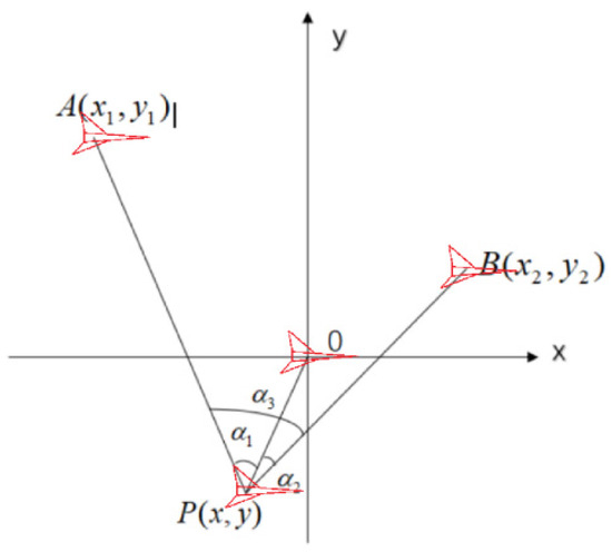
Figure 1.
Model for positioning using the center of a circle and two other points.
Furthermore, the angles between each pair of these three vectors are all known, and the equation holds. We then computed the following expressions using both coordinate-based operations and the definition of the vector dot product:
From Equations (4) and (5), we obtained:
By squaring Equations (6) and (7), we obtained a system of bivariate quartic equations. Although analytical solutions for x and y cannot be derived, numerical solutions within a defined range can be selected to approximate the true solution.
In real-world flight operations, when the UAV formation (O, A, B, P) is executing missions, the drone at point P may deviate from its intended position within the formation, necessitating autonomous repositioning through self-localization.
The UAVs at points O, A, and B transmit electromagnetic waves to the drone at point P. Upon receiving these signals, the P-positioned UAV calculates the included angles and , and then determines its coordinates P(x,y) using Equation (1). Subsequently, the P-positioned drone transmits its computed positional data to other UAVs in the formation, thereby achieving position localization and formation updates.
2.2. Analysis of Internal Electromagnetic Interference in UAV Formation Systems
EMC challenges in UAV swarms originate from inter-drone electromagnetic interference generated by individual unit radiation [23,24,25]. During cooperative target localization, inter-vehicle EM wave propagation forms intricate electromagnetic coupling networks. Given the UAV at node A transmitting electromagnetic waves to node P, we defined the spatial electromagnetic energy density according to Maxwell’s equations, where E is the electric field intensity, B is the magnetic flux density, is the vacuum permittivity, and is the vacuum permeability [26].
Referring to Figure 2, given that the UAV at node A transmits EM waves to node P, we defined e as the spatial EM energy density, and in this case, the physical meaning of e corresponds to the aforementioned [27,28,29,30].
where r represents the distance from point A to the spatial point where the electromagnetic wave energy density is measured, and denotes the electromagnetic wave energy density at unit distance.
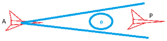
Figure 2.
Electromagnetic wave emission diagram.
In practical scenarios, when electromagnetic waves encounter medium interfaces and undergo reflection, the resulting increase in signal path length leads to energy attenuation that deviates from the ideal model. As signals arrive at the receiver through multiple paths, path differences cause phase interference, creating multi-path effects. However, in the formation environment considered in this study, where the scale is significantly smaller than reflective surfaces such as buildings and the ground, these effects can be neglected. Therefore, this model was employed.
In real-world scenarios, the UAV at point P receives multiple electromagnetic wave signals simultaneously. As illustrated in Figure 3, these signals may interfere with each other, introducing potential electromagnetic compatibility risks to the passive positioning system of the UAV.
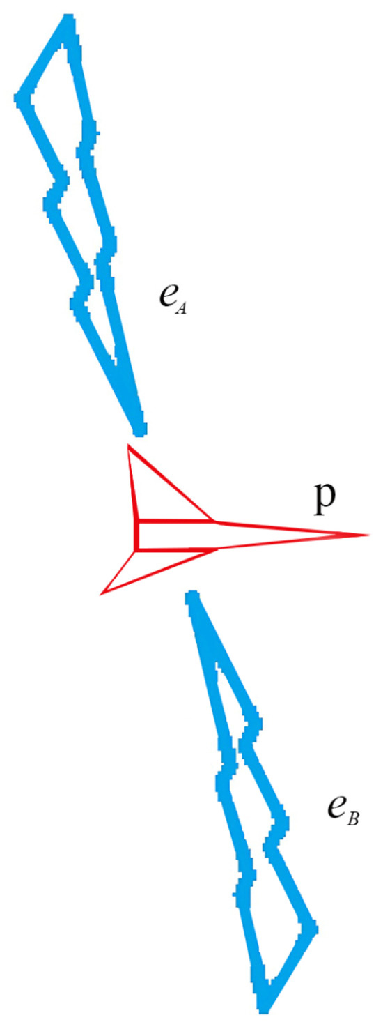
Figure 3.
Waveform diagram of received electromagnetic signals from two sources.
The following analysis explains this phenomenon from the three essential elements of electromagnetic compatibility (EMC) [31,32,33,34,35]. Since electromagnetic signals may potentially interfere with each other, when a UAV simultaneously receives two EM wave signals ( and ), considering as the primary signal, the signal effectively acts as an electromagnetic disturbance to . The specific interference relationship is detailed in Table 2.
Table 2.
List of three key elements for EMC in dual-beam scenarios.
When the UAV at point P simultaneously receives two electromagnetic wave signals and , let us assume that the energy density of signal exceeds that of (). The electromagnetic interference energy generated by signal is defined as k times its intrinsic energy, , expressed as:
In this study, we defined the electromagnetic compatibility condition as (*) to evaluate interference effects on UAV positioning accuracy when multiple electromagnetic signals are present [36,37,38]. The condition is specified in Table 3 as follows:
Table 3.
List of electromagnetic compatibility condition.
2.3. Establishment of Passive Positioning Model for UAV Formation
During formation flight missions, UAV formations maintain electromagnetic silence to avoid interference, meaning the system refrains from emitting any electromagnetic signals externally. To preserve formation geometry, a bearings-only passive positioning method was employed for UAV position adjustment. Specifically, the selected drones within the formation transmitted signals while others passively received them, extracting directional information for localization to coordinate positional adjustments.
Each drone in the formation had a fixed identification number. The drone formation consisted of 10 UAVs arranged in a centered circular formation, with 9 drones (numbered UAV01 to UAV09) evenly distributed along the same circumference and 1 central drone (numbered UAV00) located at the circle’s center (see Figure 4). All drones maintained the same flight altitude.
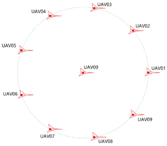
Figure 4.
Ten UAV formation pattern diagram.
According to the formation requirements, one UAV is positioned at the circle center, while the other nine UAVs are uniformly distributed on the circumference centered around UAV00. At a certain moment, the UAV positions exhibit minor deviations. An electromagnetic compatibility (EMC)-based passive positioning adjustment scheme was implemented for the drone formation. Through iterative adjustments, each UAV can be repositioned to its ideal location, ultimately ensuring the nine UAVs achieve uniform distribution on a designated circumference.
The UAV position adjustment scheme consists of three sequential steps: node selection, position adjustment, and termination judgment. First, by analyzing the positional data of all formation UAVs and their electromagnetic compatibility (EMC) when transmitting signals, three optimal UAVs are selected as signal emitters to determine the target UAV’s precise location. Then, through iterative polar coordinate calculations, deviated UAV positions are progressively corrected to their standard locations. Finally, the adjustment process terminates when verification confirms that all nine peripheral UAVs (excluding the central one) achieve approximately uniform distribution along the designated circumference.
Each UAV initially possesses polar coordinate data (radius and azimuth angle ). However, since the formation must maintain electromagnetic silence during flight, accurate GPS positioning coordinates cannot be obtained. Instead, only the angular separation between UAVs can be measured through mutual electromagnetic wave signal transmissions.
2.4. Site Selection Criteria for UAV Formations Under Internal Interference Conditions
For a specific UAV (denoted as UAV0i, i = 1,2,3…9), based on the formation system’s electromagnetic compatibility analysis, the electromagnetic wave energy density (Equation (10)) and electromagnetic interference energy density (Equation (11)) received by UAV0i can be obtained when other formation UAVs (denoted as UAV0j, j ≠ i) transmit signals to it:
Let .
If , it means the system meets the electromagnetic compatibility condition (*), and the three selected drone points used for positioning can be chosen arbitrarily.
If , then under the condition that the electromagnetic compatibility condition (*) is satisfied, the system can only select points that meet the following criteria to locate the target drone:
,
and
Among them, are the three numbers that satisfy condition .
To ensure that the final passive positioning adjustment results in a formation where 9 drones are evenly distributed on a circumference centered around UAV00, UAV00 must be selected as the reference drone for each positioning.
2.5. Passive Positioning Adjustment and Global Iteration
Adopt a sequential adjustment and overall iteration approach for the UAVs in the formation to optimize their positions, ultimately ensuring they are evenly distributed on a circle.
Select a specific UAV (assumed to be UAV0i), with the coordinates denoted as . Following the aforementioned point selection principle, use UAV00, UAV0j1, and UAV0j2 to determine its position. Define the proximity measure s:
In function , the first term represents the angle between the two electromagnetic waves received by the current UAV (UAV0i) from UAV00 and UAV0j1, while the second term denotes the angle under standard conditions (i.e., without positional deviation) between the two electromagnetic waves received by UAV0i from UAV00 and UAV0j1. In function , the first term represents the angle between the two electromagnetic waves received by UAV0i from UAV00 and UAV0j2, and the second term indicates the angle under standard conditions (i.e., without positional deviation) between the two electromagnetic waves received by UAV0i from UAV00 and UAV0j2.
When there is no positional deviation, the values of and are both zero, and the proximity measure s equals 0.
Therefore, during position adjustment, the proximity measures should be minimized as much as possible, allowing the passively signal-receiving UAV0i to approach the ideal position more closely than its original location, thereby optimizing individual positioning.
Considering that each circle has two degrees of freedom (the position of the center and the radius), UAV00 was set as the center, and the distance between UAV01 and UAV00 was defined as the radius. Except for UAV00 (which establishes the reference frame) and UAV01 (which determines the radius), all other UAVs on the circle (from UAV02 to UAV09) require positional adjustments to approach an ideal uniform distribution along the circumference. Each update of the positions of UAV02 through UAV09 is referred to as one global iteration.
For UAV formations, each global iteration brings the distribution closer to the ideal uniform state. Thus, with a sufficient number of global iterations, all UAVs will converge to bias-free accurate positions.
With electromagnetic compatibility ensured, each UAV has achieved effective positioning with determined coordinates. Taking UAV00 as the origin and the connecting line between UAV01 and UAV00 as the polar axis, a polar coordinate system is established, allowing measurement of polar radius () and polar angle (). Given the strong correlation between and , this scheme simplifies the evaluation process by considering only the polar radius ().
Since the position of the UAV transmitting the signal, which serves as the reference for point selection and positioning in this model, may have a certain deviation, even after multiple iterations, it is impossible to ensure that all points are precisely and uniformly distributed on the circumference. However, these points gradually converge toward a standard circle with a defined radius during the iterative process.
The judgment criterion was set as follows: Taking the ideal deviation-free accurate position of each UAV as the center and a fixed value as the radius, if the adjusted position fall within this circular area, the UAV was considered to have reached its ideal position.
3. Simulation and Results
3.1. Signal Transmission Methods and Specific Implementation Processes in Simulation
In the theoretical discussion above, this paper did not explicitly specify how the position of each drone was calculated. In practice, two methods were employed in simulations and experiments: centralized computation and decentralized computation, depending on the location of the processing unit. The flowcharts for centralized and decentralized computation are included in Appendix B Figure A3.
If each drone has onboard computational capabilities, every drone can independently adjust its position upon receiving angular signals. The workflow for a single drone (labeled A) is as follows.
- A receives electromagnetic waves emitted by three reference drones (B, C, D) and collects the angles between the three beams.
- A compares the current measured angles with the ideal angles at the target position.
- A adjusts its speed to alter its relative position within the formation, bringing the measured angles closer to the ideal angles.
- A completes the positional adjustment.
If only a central drone (labeled O) has computational capabilities, other drones must transmit angular data to O for processing. The workflow for a single drone (labeled A’) is as follows.
- A’ receives electromagnetic waves emitted by three reference drones (B’, C’, D’) and collects the angles between the three beams.
- A’ transmits the current measured angles to O.
- O compares the measured angles with the ideal angles at the target position through computation.
- O sends adjustment commands to A’.
- A’ adjusts its speed to alter its relative position and continuously transmits updated angles to O.
- O iteratively issues commands until the measured angles converge to the ideal angles.
- A’ completes the positional adjustment.
Notably, if the formation uses a central drone for computation, any drone in the formation can act as the central unit to handle data storage and computational tasks. Such a configuration enhances the ability to confuse adversaries and protect the system during confrontations.
3.2. Simulation Setup and Data Result Analysis
Considering specific conditions for simulation, this paper established a UAV formation based on the aforementioned passive positioning model. Under the given simulation scenario, the deviation of UAVs from their standard positions is significantly smaller than the radius of the flight formation, meaning only minor positional offsets occur. Appendix A Table A1 provides comparative simulation data between the ideal scenario (i.e., standard positions) and the initial positions with slight deviations.
When performing positioning and adjustment for the UAVs requiring calibration, the first step is to select reference points based on electromagnetic compatibility (EMC). Table 4 below presents the simulated EMC parameter data:
Table 4.
Simulation parameter data sheet.
Taking UAV002 as an example for EMC (Electromagnetic Compatibility) point selection, Appendix A Table A2 and Appendix B Figure A1 list all possible cases of positioning electromagnetic wave energy density and corresponding electromagnetic interference energy emitted by other UAVs toward UAV002.
During UAV002’s positioning and adjustment process, three UAVs must be selected as passive positioning reference points (with UAV00 being mandatory), while the second selection has eight possible options. Using UAV006 as an example, the following EMC line chart for point selection can be plotted, as shown in Figure 5.
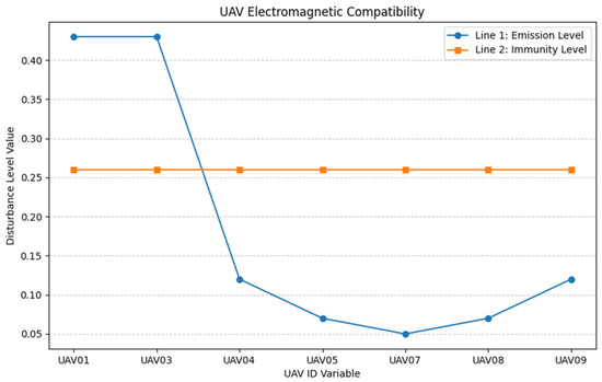
Figure 5.
Site selection electromagnetic compatibility (EMC) trade-off curve.
This study selected one of the electromagnetic compatibility-compliant configurations to perform positioning and adjustment for UAV002, with three UAVs designated as passive positioning reference points: UAV00, UAV06, and UAV07. Appendix A Table A3 provides the passive positioning matching status of other UAVs in this study.
Since the simulation process can calculate the precise position of each UAV in real time, the following equation can be used when simulating the reception angles and :
By substituting Equations (15) and (16), we obtained:
In each iteration, the UAV can search for the minimum value within a 1 m grid around itself (step size of 0.1 m). The general process of the aforementioned simulation can be expressed in pseudocode as following Algorithm 1.
| Algorithm 1. Optimizing UAV Formation Alignment Using Passive Localization Method |
| Input: Initial coordinates of each UAV Termination Condition: #In this simulation, the condition is set as all UAVs must lie within a 1 m radius circle centered at their ideal (unbiased) positions While termination condition is not met: Adjustment for UAV02 UAV02 selects a matching UAV pair for self-localization based on electromagnetic compatibility (EMC) criteria Receives three electromagnetic beams and calculates two angles Compares these angles with the reference angles at the ideal position to compute the proximity scores Adjusts its position to make the received angles closer to the reference angles Reduces the proximity score s ’’’ UAV03 to UAV09 perform similar adjustments ’’’ One iteration completes, and data are collected Check if termination condition is reached |
This paper validated the adjustment results by setting the mean values of the overall radial deviation () and the overall angular deviation (). The definitions are as follows.
Mean overall radial deviation :
Mean overall angular deviation :
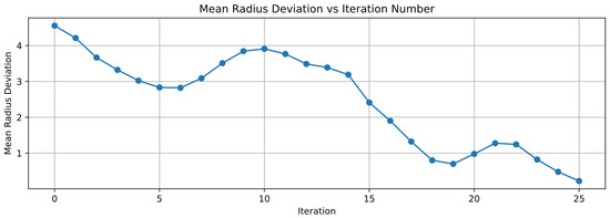
Figure 6.
Mean radial deviation vs. iteration number plot.
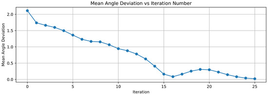
Figure 7.
Mean angular deviation vs. iteration number plot.
As can be seen from the figure, with the increase in iteration times, the mean values of polar radius deviation and polar angle deviation both show an overall decreasing trend, indicating that the passive positioning adjustment for UAV formation based on electromagnetic compatibility proposed in this paper is effective. The simulation iteration time and computational load can be found in the Ideal Condition Section of Table A4.
During the iteration process, the mean values of polar radius deviation exhibit an upward trend in two segments: from the 6th to the 10th iteration and from the 19th to the 21st iteration. This phenomenon occurs because polar radius deviation and polar angle deviation are strongly correlated. In some cases, adjustments to polar radius deviation may be compromised to optimize polar angle deviation. Notably, during the aforementioned segments where the mean polar radius deviation increases, the polar angle deviation consistently decreases. Such mutual adjustments ultimately enable the system to achieve the predefined UAV formation configuration.
3.3. Expansion Ideas for Other Formations
Assuming the drone formation adjustment strategy was designed as shown in Figure 8, this plan was transmitted to the designated cluster requiring adjustment. Within the current formation, the outermost drones (three or more) were selected and positioned on a circle. Using the aforementioned model, the angles formed at each drone’s position were calculated, and the adjustment model based on proximity reference was applied to determine and adjust the positions of all outermost drones.
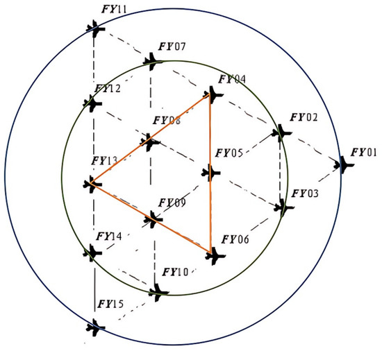
Figure 8.
Hierarchical distribution diagram of drone formation.
Next, the layer immediately inside the outermost layer, termed the target layer, was adjusted using the finalized positions of the outermost drones as reference points. By iterating this layer-by-layer inward adjustment, the entire formation gradually converged from the outer layers inward until it sufficiently approximated the ideal configuration.
4. Discussion of Real-World Deployment
For real-world deployment, we recommend employing high-gain directional antennas with selectable operating frequency bands, preferably utilizing civilian broadcast bands. High-precision azimuth measurement is achieved through an interferometric mechanism. Additionally, an Inertial Navigation Unit combining MEMS gyroscopes and accelerometers can be incorporated to enable short-term position estimation when passive positioning fails. Computational load allocation is detailed in Table 5.
Table 5.
Computational load allocation sheet.
Considering the potential uncertainties in real-world scenarios, including Gaussian noise, multi-path propagation, attenuation, directional characteristics in energy transmission, and signal distortion, this section simulates formation behavior under angular measurement errors. Based on Equation (13), we assumed deviations in the reception angle , the angle between two electromagnetic beams received by UAV02 from UAV00 and UAV06. The deviation magnitude follows a random distribution within 1%, while other conditions remain unchanged. The simulation results are as follows: Figure 9 illustrates the mean polar radius deviation versus iteration count under measurement errors, Figure 10 presents the mean polar angle deviation versus iteration count under errors, and Figure 11 displays the absolute error per measurement. Raw error data are provided in Appendix B Figure A2.
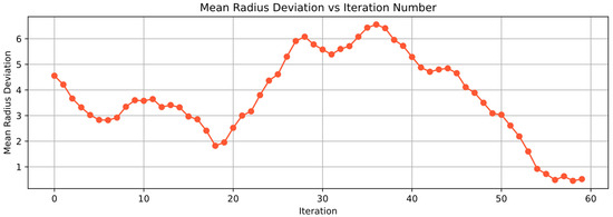
Figure 9.
Mean polar radius deviation versus iteration number under measurement errors.
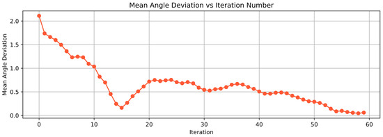
Figure 10.
Mean angular deviation versus iteration number under measurement errors.
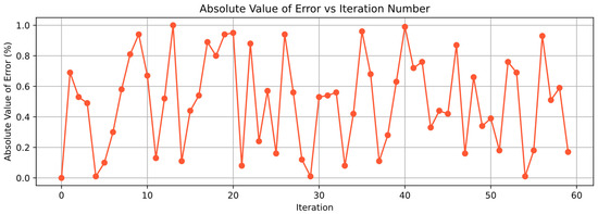
Figure 11.
Absolute error per measurement.
It is evident that significant external interference errors can adversely affect formation adjustments. As shown in the figures, around the 26th and 35th iterations—where deviation values were larger—both polar radius and polar angle deviations reached higher mean values. Conversely, around the 30th iteration, smaller deviations resulted in lower mean deviations for both the polar radius and angle, forming a trough. Overall, the mean polar radius and angle deviations asymptotically converge to zero, demonstrating the method’s robustness against interference. The simulation iteration time and computational load can be found in the With Errors Section of Table A4.
To expand the modeling scenarios for interference conditions, this paper conducted additional simulations with interference levels increased from 1% to 2%. The results demonstrate that, even after multiple iterations, the formation cannot be adjusted to the desired position. This indicates that the proposed algorithm is not applicable under strong external interference conditions.
5. Conclusions
Aiming at the electromagnetic compatibility challenges in multi-UAV formation systems, an analytical framework was proposed to quantify the electromagnetic interaction between UAV0i (i = 1, 2, 3… 9) and other formation members (UAV0j, j ≠ i). The electromagnetic wave energy density (Equation (10)) and electromagnetic interference energy density (Equation (11)) received by a designated UAV were derived based on rigorous electromagnetic compatibility analysis. By simulating scenarios with varying UAV quantities and spatial distributions, the framework demonstrated robust adaptability in evaluating intra-formation electromagnetic impacts under different operational scales. Compared with conventional single-device or non-directional interference models, the proposed dual-energy-density metric effectively characterizes both constructive signal reception and destructive electromagnetic harassment, providing critical theoretical support for optimizing formation communication topology. The results validate the framework’s reliability in ensuring electromagnetic compatibility for UAV swarms in complex environments.
When measurement errors are relatively small, the formation can still autonomously adjust to the preset configuration. However, as interference levels increase, the proposed algorithm demonstrates difficulty in achieving the desired positioning. Future work will focus on dynamic interference mitigation strategies for real-time formation reconfiguration scenarios.
Author Contributions
Methodology, J.H.; Resources, W.W.; Writing—original draft, J.H.; Writing—review & editing, L.Z.; Project administration, L.Z. All authors have read and agreed to the published version of the manuscript.
Funding
This research was funded by National Key Laboratory of Electromagnetic Energy Funding Program (Grant No. 61422172320303).
Data Availability Statement
The original contributions presented in this study are included in the article. Further inquiries can be directed to the corresponding author.
Acknowledgments
The authors declare they have not used Artificial Intelligence (AI) tools in the creation of this article.
Conflicts of Interest
The authors declare there are no conflicts of interest.
Appendix A
Table A1.
The simulation data for both ideal (standard position) and slightly deviated initial positions.
Table A1.
The simulation data for both ideal (standard position) and slightly deviated initial positions.
| Drone ID | Standard Position (ρ, θ) | Initial Position (ρ, θ) |
|---|---|---|
| UAV00 | (0, 0) | (0, 0) |
| UAV01 | (100, 0) | (100, 0) |
| UAV02 | (100, 40) | (99, 41) |
| UAV03 | (100, 80) | (102, 80) |
| UAV04 | (−100, 120) | (−105, 119) |
| UAV05 | (−100, 160) | (−97, 159) |
| UAV06 | (−100, 200) | (−108, 195) |
| UAV07 | (−100, 240) | (−105, 240) |
| UAV08 | (−100, 280) | (−98, 280) |
| UAV09 | (−100, 320) | (−112, 321) |
Table A2.
All possible scenarios of electromagnetic energy density emitted by other UAVs toward UAV002 for positioning purposes and the resulting corresponding electromagnetic interference energy. This table is calculated by electromagnetic compatibility conditions (*) mentioned at Section 2.2.
Table A2.
All possible scenarios of electromagnetic energy density emitted by other UAVs toward UAV002 for positioning purposes and the resulting corresponding electromagnetic interference energy. This table is calculated by electromagnetic compatibility conditions (*) mentioned at Section 2.2.
| R1 | UAV01 | UAV03 | UAV04 | UAV05 | UAV06 | UAV07 | UAV08 | UAV09 | |
|---|---|---|---|---|---|---|---|---|---|
| R2 | |||||||||
| UAV01 | / | √ | √ | × | × | × | × | √ | |
| UAV03 | √ | / | √ | × | × | × | × | × | |
| UAV04 | √ | √ | / | √ | √ | √ | √ | √ | |
| UAV05 | × | × | √ | / | √ | √ | √ | √ | |
| UAV06 | × | × | √ | √ | / | √ | √ | √ | |
| UAV07 | × | × | √ | √ | √ | / | √ | √ | |
| UAV08 | × | × | √ | √ | √ | √ | / | √ | |
| UAV09 | √ | √ | √ | √ | √ | √ | √ | / | |
Note: In this table, the target UAV is UAV002. Three UAVs need to be selected as passive positioning reference UAVs. UAV00 is the mandatory reference UAV, and two additional UAVs must be selected. R1 and R2 represent the two reference UAVs used for positioning. The symbol √ indicates that the combination of reference UAVs meets the electromagnetic compatibility (EMC) conditions (*), while × indicates that the combination of the target UAV and reference UAVs does not meet the EMC conditions (*). The specific numerical calculations are shown in Figure A1.
Table A3.
Passive positioning matching scenarios of UAVs in this paper.
Table A3.
Passive positioning matching scenarios of UAVs in this paper.
| Target UAV | Passive Positioning Reference UAV |
|---|---|
| UAV02 | UAV00, UAV06, UAV07 |
| UAV03 | UAV00, UAV07, UAV08 |
| UAV04 | UAV00, UAV08, UAV09 |
| UAV05 | UAV00, UAV01, UAV09 |
| UAV06 | UAV00, UAV01, UAV02 |
| UAV07 | UAV00, UAV02, UAV03 |
| UAV08 | UAV00, UAV03, UAV03 |
| UAV09 | UAV00, UAV04, UAV05 |
Table A4.
Comparison table of simulation iteration time and computational load.
Table A4.
Comparison table of simulation iteration time and computational load.
| Scenario | Iteration Time (s) | CPU Utilization (%) 1 |
|---|---|---|
| Ideal Condition | 0.117727 | 3.9 |
| With Errors | 0.270794 | 5.2 |
1 The CPU model used for simulation was 12th Gen Intel (R) Core (TM) i5-12500H 2.50 GHz.
Appendix B
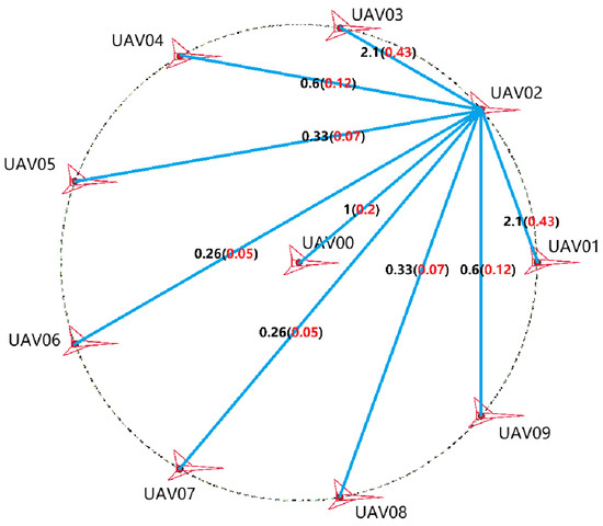
Figure A1.
Figure of numerical values for the electromagnetic wave energy density emitted by other UAVs to UAV002 for positioning and the corresponding electromagnetic interference energy generated. Note: In this figure, the blue lines represent the electromagnetic beams, the black numbers along the blue lines indicate the electromagnetic wave energy density calculated using Equation (10), and the red numbers indicate the electromagnetic interference energy calculated using Equation (11).
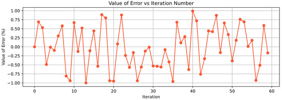
Figure A2.
Value of error per measurement.
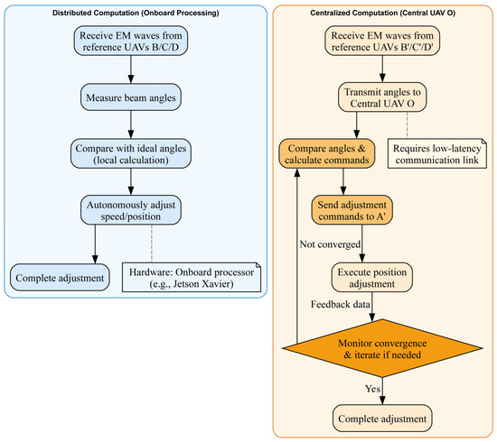
Figure A3.
The flowcharts for centralized and decentralized computation. Note: The flowchart clearly demonstrates strong interdependencies among drones within the formation. When any single drone malfunctions, the system becomes incapable of maintaining the original positioning strategy and must immediately switch to an alternative positioning approach. Failure to do so would cause the formation to deviate significantly from its intended relative positioning.
References
- Karthigesu, J.; Owari, T.; Tsuyuki, S.; Hiroshima, T. UAV Photogrammetry for Estimating Stand Parameters of an Old Japanese Larch Plantation Using Different Filtering Methods at Two Flight Altitudes. Sensors 2023, 23, 9907. [Google Scholar] [CrossRef] [PubMed]
- Mohsan, S.A.H.; Khan, M.A.; Alsharif, M.H.; Uthansakul, P.; Solyman, A.A.A. Intelligent Reflecting Surfaces Assisted UAV Communications for Massive Networks: Current Trends, Challenges, and Research Directions. Sensors 2022, 22, 5278. [Google Scholar] [CrossRef] [PubMed]
- Arif, M.; Kim, W.; Iqbal, A.; Kim, S.W. Analysis of MCP-Distributed Jammers and 3D Beam-Width Variations for UAV-Assisted C-V2X Millimeter-Wave Communications. Mathematics 2025, 13, 1665. [Google Scholar] [CrossRef]
- Xu, G.; Shi, Y.; Sun, X.; Shen, W. Internet of Things in Marine Environment Monitoring: A Review. Sensors 2019, 19, 1711. [Google Scholar] [CrossRef]
- Wang, Z.; Zhang, Z.; Dou, W.; Hu, G.; Zhang, L.; Zhang, M. Extending Conflict-Based Search for Optimal and Efficient Quadrotor Swarm Motion Planning. Drones 2024, 8, 719. [Google Scholar] [CrossRef]
- Liu, F.; Li, M.; Guo, L.; Guo, H.; Cao, J.; Zhao, W.; Wang, J. Edge-Deployed Band-Split Rotary Position Encoding Transformer for Ultra-Low-Signal-to-Noise-Ratio Unmanned Aerial Vehicle Speech Enhancement. Drones 2025, 9, 386. [Google Scholar] [CrossRef]
- Ohkawa, S.; Ueda, K.; Miyoshi, T.; Yamazaki, T.; Yamamoto, R.; Funabiki, N. Relay Node Selection Methods for UAV Navigation Route Constructions in Wireless Multi-Hop Network Using Smart Meter Devices. Information 2025, 16, 22. [Google Scholar] [CrossRef]
- Ntousis, O.; Makris, E.; Tsanakas, P.; Pavlatos, C. A Dual-Stage Processing Architecture for Unmanned Aerial Vehicle Object Detection and Tracking Using Lightweight Onboard and Ground Server Computations. Technologies 2025, 13, 35. [Google Scholar] [CrossRef]
- Yan, X.; Wang, J.; Wu, F.; Bai, J.; Zhang, X.; Li, G.; Fei, H. Spatial and Temporal Variation Characteristics of Air Pollutants in Coastal Areas of China: From Satellite Perspective. Remote Sens. 2025, 17, 1861. [Google Scholar] [CrossRef]
- Tao, C.; Liu, B. Distributed coordinated motion control of multiple UAVs oriented to optimization of air-ground relay network. Sci. Rep. 2024, 14, 23920. [Google Scholar] [CrossRef]
- Galimov, M.; Fedorenko, R.; Klimchik, A. UAV Positioning Mechanisms in Landing Stations: Classification and Engineering Design Review. Sensors 2020, 20, 3648. [Google Scholar] [CrossRef] [PubMed]
- Zeng, Y.; Zhang, R.; Lim, T.J. Throughput Maximization for UAV-Enabled Mobile Relaying Systems. IEEE Trans. Commun. 2016, 64, 4983–4996. [Google Scholar] [CrossRef]
- Fonseca, E.; Galkin, B.; Amer, R.; DaSilva, L.A.; Dusparic, I. Adaptive Height Optimization for Cellular-Connected UAVs: A Deep Reinforcement Learning Approach. IEEE Access 2023, 11, 5966–5980. [Google Scholar] [CrossRef]
- Azari, M.M.; Geraci, G.; Garcia-Rodriguez, A.; Pollin, S. UAV-to-UAV Communications in Cellular Networks. IEEE Trans. Wirel. Commun. 2020, 19, 6130–6144. [Google Scholar] [CrossRef]
- Xiao, Z.; Liu, K.; Zhu, L. Millimeter-wave array enabled UAV-to-UAV communication technology. J. Commun. 2022, 43, 3–13. [Google Scholar]
- Feng, R.; Wu, W.; Qian, L.; Chang, Y.; Yousaf, M.Z.; Khan, B.; Aierken, P. A Hybrid TDOA and AOA Visible Light Indoor Localization Method Using IRS. Electronics 2025, 14, 2158. [Google Scholar] [CrossRef]
- Guo, J.; Wang, Y. Efficient AOA Estimation and NLOS Signal Utilization for LEO Constellation-Based Positioning Using Satellite Ephemeris Information. Appl. Sci. 2025, 15, 1080. [Google Scholar] [CrossRef]
- Shen, B.; Chen, J.; Xu, G.; Chen, Q.; Wang, J. Performance Analysis of a Drone-Assisted FSO Communication System over Málaga Turbulence under AoA Fluctuations. Drones 2023, 7, 374. [Google Scholar] [CrossRef]
- Xue, J.; Su, B.; Liu, Y.; Meng, J. A Multi-Receiver Pulse Deinterleaving Method Based on SSC-DBSCAN and TDOA Mapping. Electronics 2025, 14, 1833. [Google Scholar] [CrossRef]
- Wei, S.; Tang, H.; Liu, C.; Yang, T.; Zhou, X.; Zlatanova, S.; Fan, J.; Tu, L.; Mao, Y. DeepLabV3+-Based Semantic Annotation Refinement for SLAM in Indoor Environments. Sensors 2025, 25, 3344. [Google Scholar] [CrossRef]
- Heshmat, M.; Saad Saoud, L.; Abujabal, M.; Sultan, A.; Elmezain, M.; Seneviratne, L.; Hussain, I. Underwater SLAM Meets Deep Learning: Challenges, Multi-Sensor Integration, and Future Directions. Sensors 2025, 25, 3258. [Google Scholar] [CrossRef]
- Yao, F.; Zhu, Y.; Sun, Y.; Guo, W. Wireless communications “N+1 dimensionality” endogenous anti-jamming: Theory and techniques. Secur. Saf. 2023, 3, 29–43. [Google Scholar] [CrossRef]
- Esmaeilkhah, A.; Landry, R.J. Estimation of the Effect of Single Source of RF Interference on an Airborne Global Navigation Satellite System Receiver: A Theoretical Study and Parametric Simulation. Eng. Proc. 2025, 88, 53. [Google Scholar] [CrossRef]
- Sun, X.; Zhang, J.; Wang, W.; He, D. A Wearable Dual-Band Magnetoelectric Dipole Rectenna for Radio Frequency Energy Harvesting. Electronics 2025, 14, 1314. [Google Scholar] [CrossRef]
- Ye, M.; Wang, W.; Jia, J.; Cai, W.; Cao, Q.; Sheng, K. Research on an Electromagnetic Compatibility Test Method for Connected Automotive Communication Antennas. Sensors 2025, 25, 1922. [Google Scholar] [CrossRef] [PubMed]
- Barclay, B.M.; Kostelich, E.J.; Mahalov, A. Vectorial EM Propagation Governed by the 3D Stochastic Maxwell Vector Wave Equation in Stratified Layers. Atmosphere 2023, 14, 1451. [Google Scholar] [CrossRef]
- Huang, K.; Xiao, Q.; Chen, J.; Dong, M. A Study on the Electromagnetic Characteristics of Very-Low-Frequency Waves in the Ionosphere Based on FDTD. Electronics 2025, 14, 1545. [Google Scholar] [CrossRef]
- Zhao, L.; Zhan, Z.; Zhang, Z.; Feng, H. Analysis of VLF Electromagnetic Scattering in Lower Anisotropic Ionosphere Based on Transfer Matrix. Atmosphere 2024, 15, 1396. [Google Scholar] [CrossRef]
- Barbosa, B.S.d.S.; Cruz, H.A.O.; Macedo, A.S.; Cardoso, C.M.M.; Fernandes, F.C.; Eras, L.E.C.; Araújo, J.P.L.d.; Calvacante, G.P.S.; Barros, F.J.B. Application of Artificial Neural Networks for Prediction of Received Signal Strength Indication and Signal-to-Noise Ratio in Amazonian Wooded Environments. Sensors 2024, 24, 2542. [Google Scholar] [CrossRef]
- Zhang, Y.; Zhang, F.; Wang, Z.; Zhang, X. Localization Uncertainty Estimation for Autonomous Underwater Vehicle Navigation. J. Mar. Sci. Eng. 2023, 11, 1540. [Google Scholar] [CrossRef]
- Garczarek, A.; Stachowiak, D. Measurements and Analysis of Electromagnetic Compatibility of Railway Rolling Stock with Train Detection Systems Using Track Circuits. Energies 2025, 18, 2705. [Google Scholar] [CrossRef]
- Gavai, A.; Gope, D.; Dhoot, V.; Hansen, J. Probabilistic Characterization and Machine Learning-Based Modeling of Conducted Emissions of Programmable Microcontrollers. Electronics 2025, 14, 1511. [Google Scholar] [CrossRef]
- Bashkeev, A.; Parshin, A.; Trofimov, I.; Bukhalov, S.; Prokhorov, D.; Grebenkin, N. Modern Capabilities of Semi-Airborne UAV-TEM Technology on the Example of Studying the Geological Structure of the Uranium Paleovalley. Minerals 2025, 15, 630. [Google Scholar] [CrossRef]
- Illiano, L.; Liu, X.; Wu, X.; Grassi, F.; Pignari, S.A. Signal Order Optimization of Interconnects Enabling High Electromagnetic Compatibility Performance in Modern Electrical Systems. Energies 2024, 17, 2786. [Google Scholar] [CrossRef]
- Xi, Y.-Z.; Liao, G.-X.; Lu, N.; Li, Y.-B.; Wu, S. Study on the Aeromagnetic System between Fixed-Wing UAV and Unmanned Helicopter. Minerals 2023, 13, 700. [Google Scholar] [CrossRef]
- Cai, J.; Li, J.; Xie, S.; Jin, H. Evaluation and Anomaly Detection Methods for Broadcast Ephemeris Time Series in the BeiDou Navigation Satellite System. Sensors 2024, 24, 8003. [Google Scholar] [CrossRef]
- Chen, X.; Xie, S.; Wei, M.; Yang, Y. A Study on the Frequency-Domain Black-Box Modeling Method for the Nonlinear Behavioral Level Conduction Immunity of Integrated Circuits Based on X-Parameter Theory. Micromachines 2024, 15, 658. [Google Scholar] [CrossRef]
- Ma, Z.; Wei, H.; Yuan, X. A Novel Transfer Function Model Based on the Feature Selection Validation Method for Quadrotor Unmanned Aerial Vehicles in High-Intensity Radiated Field Environments. Electronics 2025, 14, 976. [Google Scholar] [CrossRef]
Disclaimer/Publisher’s Note: The statements, opinions and data contained in all publications are solely those of the individual author(s) and contributor(s) and not of MDPI and/or the editor(s). MDPI and/or the editor(s) disclaim responsibility for any injury to people or property resulting from any ideas, methods, instructions or products referred to in the content. |
© 2025 by the authors. Licensee MDPI, Basel, Switzerland. This article is an open access article distributed under the terms and conditions of the Creative Commons Attribution (CC BY) license (https://creativecommons.org/licenses/by/4.0/).