Highlights
What are the main findings?
- A Stochastic Microscale Wind Model (SWM) has been developed and validated to support the operation and certification flight testing of Urban Air Mobility (UAM) aircraft, including drones, RPAs, and piloted VTOL vehicles.
- SWM can rapidly generate high-resolution, quasi-non-stationary urban wind fields, delivering mid-fidelity performance that bridges the gap between spectral models and CFD-based approaches.
What is the implication of the main finding?
- SWM delivers realistic, low-cost microscale wind simulations using open-source terrain data and standard wind solvers, with straightforward mesoscale integration and a clear pathway toward real-time wind prediction.
- SWM-generated wind data can support preliminary flight dynamics, performance, control, safety, and operational risk assessments for drones and VTOL aircraft, as well as vertiport siting studies, helping accelerate the development and deployment of UAM.
Abstract
Urban air mobility operations, such as flying Uncrewed Aerial Vehicles (UAVs) and small passenger aircraft in and around cities, will be inherently susceptible to the turbulent wind conditions in urban environments. Therefore, understanding UAM aircraft performance under microscale wind disturbances is critical. Gaining such insight is non-trivial due to the lack of sufficient UAM aircraft operational data and the complexities involved in flight testing UAM aircraft. A viable solution to overcome this hindrance is through simulation-based flight testing, data collection, and performance assessment. To support this effort, the present paper establishes a custom Stochastic microscale Wind Model (SWM) capable of efficiently generating high-resolution, spatio-temporally varying urban wind fields. The SWM is validated against wind tunnel test data, and subsequently, the findings are employed to guide targeted refinements of urban wake simulation. Furthermore, to incorporate realistic atmospheric conditions and demonstrate the ability to generate location-specific wind fields, the SWM is coupled with the mesoscale Weather Research and Forecasting (WRF) model. This integrated approach is demonstrated through a case study focused on a potential vertiport site in Milan, Italy, illustrating its utility for assessing operational area-specific UAM aircraft performance and vertiport emplacement.
1. Introduction
Urban Air Mobility is a new mode of air transport system technology driven by the need for sustainable mobility options to tackle road traffic congestion and improve connectivity in and around cities. In general, the term “UAM aircraft” refers to crewed, autonomous, or semi-autonomous electric Vertical Takeoff and Landing (eVTOL) aircraft, such as UAVs and small passenger aircraft, that are specifically designed to operate at low altitudes over urban areas for both passenger and cargo transportation.
As of October 2024, there are over 52 UAM aircraft manufacturers worldwide [1]. All of these firms have one or more aircraft prototypes (or designs) to facilitate UAM missions such as airport shuttle, delivery, and on-demand services. However, none of these solutions is still available on the market. This can be attributed, in part, to the fact that, unlike traditional helicopters and aircraft, UAM vehicles leverage distributed propulsion and autonomous technologies, enabling operations in regions underserved by other modes of transport [2]. These characteristics, when combined with the diverse configurations and light-weight of UAM aircraft, elevate the aerodynamic nonlinearity and overall system complexity [3], leading to the introduction of safety and performance deviation risks that are currently unknown to the aviation sector.
In addition to the challenges associated with vehicle technology, a major and pervasive obstacle for UAM operations lies in the microscale wind conditions of the environments in which they must operate [4,5]. That is, UAM operations—particularly crucial flight phases such as take-off, landing, and approach—are intended to be conducted within the Urban Boundary Layer (UBL) or low-altitude atmosphere [6,7,8], where wind flow is continuously disrupted by buildings and structures, resulting in high-intensity turbulence and complex flow regions. Such wind flow patterns will significantly affect UAM aircraft performance, amplifying operational and ground safety risks such as trajectory deviations, collisions, injuries or fatalities, vehicle or property damage, and financial loss. These intricacies—arising from both vehicle technology and urban atmospheric conditions—pose a barrier to UAM aircraft certification as they demand more time, effort, financial investment, and meticulous risk mitigation strategies, rendering safe flight testing in urban airspace increasingly elusive. Nonetheless, it is of utmost importance to characterize, evaluate, and assess urban microscale wind-induced aircraft performance deviation for the safe realization of UAM.
A commonly used alternative to flight testing is based on leveraging historical operational data for aircraft performance evaluation and risk analysis [9]. Unfortunately, this approach is unfeasible for UAM, as no such vehicles currently operate over densely populated urban areas. This constraint is also emphasized in the Means of Compliance with the Special Condition for Vertical Take-Off and Landing (SC-VTOL) aircraft, published by the European Union Aviation Safety Agency (EASA), which notes that the absence of urban flight performance data limits detailed understanding of Atmospheric Disturbance (AD) levels for UAM aircraft [10]. On the whole, among traditional aircraft performance assessment techniques—flight testing, operational data analysis, and analytical modeling [11]—simulation-based frameworks presently represent the only efficient means to address microscale wind-induced challenges in performance assessment, certification, and safe integration of UAM systems.
Within simulation-based performance assessment frameworks for conventional aircraft, AD is typically incorporated using real-time sensor data, archived meteorological records, or validated wind models designed to replicate gusts and turbulence in the high-altitude atmosphere [12]. These strategies are unsuitable for UAM due to the impracticality of sensor placement in UBL, the lack of low-altitude observational wind data, and inability of standardized models to accurately represent urban wind gusts. Therefore, wind models that explicitly account for the influence of buildings and urban structures are essential to accurately capture the complex microscale wind dynamics for UAM. In recognition of this need, the authors recently published a comprehensive review article that catalogs several urban wind modeling techniques, presents statistical evidence on the existing knowledge gap within the UAM community regarding microscale weather, and underscores the importance of making informed decisions when choosing wind models for different UAM applications [13]. One of the key outcomes from the review was that most existing research employs either spectral methods (Von Kármán or Dryden) or hybrid modeling approaches, where Computational Fluid Dynamic (CFD) techniques are combined with historical data, statistical methods such as machine learning, or mesoscale models. While these models offer flexibility, they often trade off between accuracy and computational cost—i.e., they either oversimplify urban wind conditions to reduce computational burden or incur significant computational expense to achieve higher fidelity.
Building on these findings, and considering the unique characteristics of UAM—such as smaller aircraft dimensions, limited flight durations due to current battery constraints, and the need for rapid wind data generation to support applications like aircraft performance assessment [14]—this paper introduces a custom wind model, SWM, designed to balance fidelity with computational efficiency. This paper also illustrates the validation of the SWM by replicating wind tunnel test scenarios derived from existing literature. Simulation results are compared against corresponding experimental data to assess model accuracy and guide refinement of the SWM. As a secondary objective, the paper couples the SWM with the Weather Research and Forecasting (WRF) model to enhance the realism of the SWM and capture the dynamic interactions between the mesoscale atmospheric flows on the microscale wind conditions (see Figure 1). This integrated WRF–SWM framework is illustrated by a case study in a selected area of Milan, Italy, to showcase SWM’s capability to support research on vertiport emplacement and aircraft performance assessment in the region.
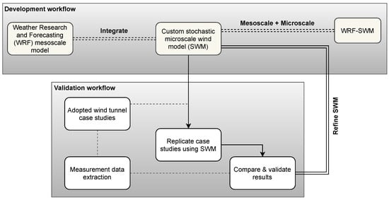
Figure 1.
SWM development and validation workflow chart.
The paper is organized as follows: Section 2 introduces the SWM framework. Section 3 describes the validation setup and evaluates SWM’s performance against three wind tunnel scenarios of increasing geometric complexity. Section 4 integrates SWM with the mesoscale WRF model and presents a case study for a potential vertiport site in Milan. Finally, Section 5 concludes with key findings and future research directions.
2. Overview of Custom Stochastic Microscale Wind Model
Atmospheric properties like wind speed and temperature exhibit the steepest gradients at low altitude (<2 km) due to the complexity of urban terrain [15]. Turbulence and its spectra are also highly dynamic, with scales and intensity fluctuating locally at a high frequency due to thermal instabilities caused by urban topography [16]. This behavior contrasts with the more stable conditions observed at higher altitudes, where topographical influence on wind flow is minimal. Consequently, the mesoscale models used for high-altitude wind prediction in the commercial aviation sector are unsuitable for UAM applications. Therefore, in the following, a custom microscale wind model, SWM, is developed.
The SWM is based on Reynolds decomposition, where the total velocity field U is separated into steady () and unsteady () components [17,18], namely:
Here, denotes the velocity component in the X-, Y-, or Z-direction (i.e., and w, respectively); i, j, and k are the discrete spatial indices in the streamwise (X), lateral (Y), and vertical (Z) directions in a Cartesian coordinate system; and n is the time step index.
To synthesize the steady and unsteady components of wind velocity, the SWM implicitly integrates a highly parameterized steady-state wind solver, QUIC-URB (Quick Urban and Industrial Complex—URBan) [19], with a turbulence generator, TurbSim [20]. QUIC-URB is a component of the QUIC dispersion modeling system developed by scientists at Los Alamos National Laboratory. QUIC is primarily used to estimate pollutant transport and dispersion over urban environments with high spatial resolution and computational efficiency. It is an empirical diagnostic wind solver, meaning its calculations are based on experimental observations rather than first-principle physics. QUIC-URB incorporates concepts from [21] to empirically parameterize various urban flow regions (see Figure 2). It uses obstacle geometry (length L, width W, and height H), along with inlet wind direction and speed, to estimate wind velocity fields. Vortex sizes in flow zones are determined by constraining empirical relationships to maintain mass consistency [22]. The solver produces steady-state 3D wind fields, , representing neutral atmospheric boundary layer (ABL) conditions for high-resolution domains, typically within seconds to minutes on standard desktop or laptop computers. Although evaluations have identified some discrepancies, QUIC-URB delivers CFD-like results while offering a favorable balance between resolution, speed, and accuracy [23,24,25].
On the other hand, TurbSim is a stochastic, full-field inflow turbulence generator developed by researchers at the National Renewable Energy Laboratory (NREL). It is predominantly used to determine dynamic loads on wind turbine rotors. A key feature that distinguishes TurbSim from other turbulence generators is its ability to produce turbulent velocity fields that reflect the spatiotemporal instabilities of the nocturnal boundary layer flows at low altitudes. TurbSim also offers users the flexibility to select from a variety of wind profiles (among others power, log, custom profile) and spectral models (such as Von Kármán, Kaimal, and user-defined). However, it must be noted that the TurbSim is limited to simulating turbulence velocity data () for a 2D (YZ) vertical plane [26]. Hence, within the SWM framework, to obtain turbulent velocity fields for a 3D simulation domain, TurbSim is executed multiple times at discrete streamwise (X) locations.

Figure 2.
Flow region parameterization in XY and XZ planes around an obstacle by QUIC-URB [27].
Figure 3 presents a conceptual visualization of the SWM framework, illustrating the modular combination of QUIC-URB and TurbSim to generate turbulent velocity fields. The QUIC-URB simulation domain encompasses the entire Area of Interest (AOI) and accounts for all the buildings/obstacles/structures contained within it, whereas the 2D TurbSim planes and domains are constrained to specific locations or Regions of Interest (ROI) within the AOI—such as the wake region of the building, or rooftop areas, where the Final Approach and Take-Off (FATO) zone and Safety Area (SA) are intended to be located as per the existing Vertiport standards and UAM Concept of Operations (ConOps) [28,29]. This selective application of TurbSim is strategically implemented to reduce computational time and expense, as limiting the simulation domain to only the ROIs allows for finer spatio-temporal resolution without the excessive computational demands associated with high-resolution modeling of the entire AOI.
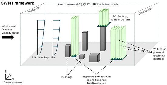
Figure 3.
Pictorial representation of SWM showing the coupled use of QUIC-URB and TurbSim.
As depicted in Figure 4, the first step in the SWM framework is to execute QUIC-URB, using the initial parameters—reference wind speed, direction, and inlet velocity profile—for steady state wind data generation across the AOI. This process yields the mean wind field , where are AOI grid indices in and direction, respectively. Then, a specific ROI, defined by grid indices along the and direction, is chosen within the AOI and its steady wind velocity data are extracted using spatial filtering of the steady-state wind field over the AOI, as follows:
where are AOI indices corresponding to .
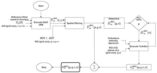
Figure 4.
Flowchart showing the steps involved in the SWM framework.
Subsequently, the filtered data are utilized to determine the mean velocity magnitude profile () for each YZ cross-sectional plane within the ROI by averaging the velocity magnitudes along the Y-axis:
where the magnitude is as follows:
The 1D mean velocity profiles ( for each p), along with other input parameters such as turbulence intensity (TI), spectrum, simulation timestep, and grid resolution, serve as inputs to repeatedly execute TurbSim for each YZ plane. This approach yields a series of YZ fluctuating velocity fields at discrete time n and X-direction. These fields are then coherently assembled across the X and time dimensions to construct an approximate spatio-temporal turbulent velocity field (). Finally, the steady mean velocity components from QUIC-URB and the turbulent fluctuations from Turbsim are superimposed to obtain the time-resolved turbulent velocity field for the ROI as follows:
A notable non-technical challenge associated with this new approach is that QUIC-URB is not open source. To use QUIC, users must obtain a license from the QUIC Team at Los Alamos National Laboratory. Although the licensing process is straightforward, it might introduce some administrative complications. Thus, as an alternative to QUIC-URB, the authors investigated the use of QES (Quick Environmental Simulation)-Winds [30,31], an open-source derivative of QUIC. The investigation revealed that QES demonstrates strong potential for UAM applications, despite its varying performance across different test scenarios. However, a limitation identified with QES is its inability to simulate wind flow fields over complex geometries whose L and W vary with H (e.g., stacked objects like buildings). Nonetheless, updates to the software and algorithms could enhance the capabilities of QES, making it a viable alternative to QUIC-URB in this novel microscale wind modeling approach. For further details on the assessment study performed by the authors on QES for UAM applications, readers are encouraged to refer to [27].
3. SWM Validation Using Wind Tunnel Case Studies and Measurements
A total of three test scenarios (TS1, TS2, and TS3) are reproduced to validate the SWM framework presented in Section 2:
- TS1 recreates the experiments by Meng and Hibi [32], conducted in a reflow wind tunnel using split fiber probes to study flow over an isolated cuboid representing an tall building.
- TS2 is derived from the PhD thesis of Neda Taymourtash [33], who employed an ABL wind tunnel and Particle Image Velocimetry (PIV) to measure time-averaged wind velocity components over a simplified frigate model representing a stacked building configuration.
- TS3 follows the setup by Cheng et al. [34], which investigated wind flow over urban topographies using randomly arranged building blocks in a low-speed open-circuit wind tunnel, with measurements obtained via hot-wire anemometry.
Overall, TS1 and TS2 are chosen to represent simplified scenarios involving flow over an isolated tall building and a ship-shaped or stacked structure, respectively. TS3 is chosen to demonstrate and evaluate the capability of the SWM framework in simulating wind flow over a complex, multi-building, urban-like configuration. Collectively, these scenarios aim to provide a comprehensive evaluation of the SWM framework’s applicability across varying degrees of geometric complexity and flow conditions.
3.1. SWM Simulation Configuration for Replication
As outlined earlier, the simulations replicate the referenced wind tunnel test scenarios to ensure fidelity in reproducing and comparing the wind velocity fields. In the present study, however, the test object dimensions and geometries for TS1, TS2, and TS3 within the SWM domain are rescaled to full size to enable a more accurate prediction and representation of turbulence structures.
Figure 5 illustrates the isometric and top views of the overall SWM domain for each test scenario. In TS1, the computational domain (or AOI) uses a uniform Cartesian grid. A rectangular building model from [32], scaled up by a factor of 500 to full scale, with an aspect ratio of , is positioned at an offset from the domain origin. The region downstream of the building, indicated by green stripes in Figure 5, is designated as the ROI, or TurbSim domain, for turbulent wind flow field generation. Within this ROI, 50 TurbSim planes are spaced along the X-axis.
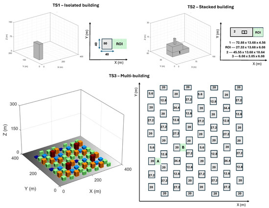
Figure 5.
SWM Domains with test object dimensions and ROI (or TurbSim domains in striped green) for TS1, TS2, and TS3. In the TS3 domain, the cuboids represent individual buildings, colour-coded by height, and the labels A and B indicate the two ROIs.
The AOI for TS2 uses a finer grid resolution. The target structure (a model of a Frigate ship used in [33], up-scaled to full size by a factor of 12.5) comprises three vertically stacked rectangular segments—namely the base, mid, and mast layers—whose dimensions are detailed in Figure 5. The ROI is defined in the wake of the mid segment (the ship deck or landing platform). To simulate the spatiotemporal evolution of the wind flow field within this ROI, 54 planes are placed at intervals along the streamwise direction. Additionally, TS2 comprises four sub-cases that share the same domain geometry and configuration but differ in inlet wind conditions to investigate the performance of SWM for varying wind speeds and directions.
Unlike TS1 and TS2, TS3 features a staggered array of 64 buildings from [34,35], scaled up by a factor of 2000. The array is placed within a large AOI, and discretized using a uniform Cartesian grid. Each building has a footprint with uniform spacing between array elements. The building heights vary randomly across five distinct values, contributing to vertical heterogeneity over a repeating unit area. The ROIs are chosen as the rear wake regions of two specific buildings (A and B) of height within the array, as depicted in Figure 5. Both ROI sections are divided into 20 YZ TurbSim planes. For further details see Table 1 and Table 2, which present a comprehensive compilation of input parameters and boundary conditions employed to generate the steady state and turbulent wind field using QUIC-URB and TurbSim within the SWM framework.

Table 1.
Key input parameters and boundary conditions used in QUIC-URB (steady) wind simulations for TS1, TS2, and TS3.
Table 2.
Key input parameters and boundary conditions used in TurbSim (unsteady) wind simulations for TS1, TS2, and TS3.
3.2. SWM Performance Validation
To ensure consistency and to mirror the results analysis presented in the referenced studies, the SWM simulation results for TS1, TS2, and TS3 are examined only at selected planes and points within the simulation domain. The adopted analysis planes intersect key flow regions around the test object, allowing for a detailed examination of the SWM performance in both near- and far-field regions, characterized by features such as upwind flow, rooftop shear layers, leeside, side, and far wakes. Overall, the evaluation focuses on two performance metrics: accuracy and computation time.
Accuracy is assessed using qualitative and quantitative approaches: qualitatively, by visually comparing flow patterns and velocity profiles; and quantitatively, using three statistical indicators—Mean Relative Error (MRE), Root Mean Square Error (RMSE), and Bias. The computation time is recorded separately for each test case to evaluate model efficiency. These performance metrics are chosen to reflect the conflicting demands of urban wind modeling for UAM applications, where achieving both computational speed and predictive accuracy is a fundamental challenge.
All three test cases are simulated on a standard laptop equipped with an 11th Gen Intel processor featuring four cores, 16 GB RAM, and a base speed of 2.80 GHz. For TS2, validation is limited to steady-state data due to the lack of unsteady wind measurements.
3.2.1. TS1 Isolated Building-Results Analysis
Figure 6 shows the analysis planes, while Figure 7 compares wind tunnel measurements and QUIC-URB predictions of steady-state wind velocity magnitude profiles for TS1. In the upwind region (), rooftop ( to ), and leeside vortex zones (–), vertical profiles show good agreement (see Figure 7a), indicating that QUIC reliably captures vertical velocity distribution and shear. In contrast, lateral profiles exhibit slight over-prediction near the ground and rooftop height (see Figure 7b,c), suggesting weaker accuracy in representing crosswind variability.
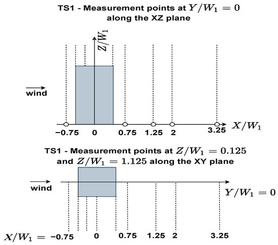
Figure 6.
TS1 measurement planes.
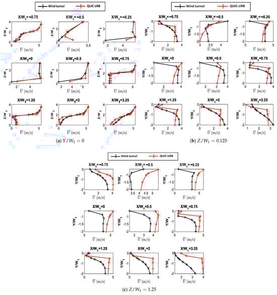
Figure 7.
TS1-Wind tunnel measurements vs. QUIC-URB velocity magnitude comparison at XZ and XY planes.
The qualitative observations made from Figure 7 are further corroborated by the quantitative error analysis summarized in Table 3. The MRE remains below 0.12, indicating that the QUIC-simulated velocities deviate by less than 12% compared to wind tunnel measurements. Similarly, the RMSE does not exceed 1.5 m/s, and the Bias remains close to zero for the upwind and leeside far wake regions, while it is around 0.3 for the rooftop and leeside near wake, supporting that vertical velocity variations across all wind flow zones are in strong agreement with experimental data. On the other hand, the MRE for lateral profiles near the ground in the wake region points to a slightly higher deviation of about 20%. The RMSE for these lateral profiles peaks at around 2.2 m/s in the leeside vortex region, while the Bias reaches approximately 0.5 in the side vortex and leeside near wake regions. More notably, QUIC substantially over-predicts the lateral profiles near rooftop height, with MRE exceeding 30%, RMSE peaking at around 3 m/s in the leeside wake, and Bias values greater than 1 across all zones. This indicates that QUIC’s ability to represent lateral flow variability—particularly near rooftop height and in wake-dominated regions—remains limited, likely due to its simplified treatment of lateral boundary conditions. Moreover, these findings are consistent with the results reported in [41], reinforcing the recognized limitations of QUIC in predicting lateral wake structures.
Table 3.
Statistical error metrics for steady-state velocity magnitude simulated by QUIC.
Figure 8 compares the standard deviation () of velocity fluctuations obtained from experiments and TurbSim for the streamwise (u), lateral (v), and vertical (w) wind components across the vertical (Z) and lateral (Y) axes. In the experimental data, the turbulence fields display coherent anisotropic structures, with dominating in magnitude but varying strongly with both height and downstream position. In the near wake, elevated values are concentrated around and slightly above building height, consistent with shear-layer roll-up and vortex shedding, whereas in the far wake the distribution broadens. Vertical gradients are pronounced, with rapid decay of above the wake core. The lateral and vertical components also show structured variability: is asymmetric across the spanwise direction, indicative of lateral shear, while exhibits localized maxima near building height, reflecting vertical recirculation and upwash/downwash motions [32,42,43].
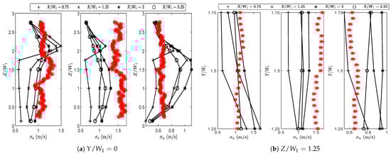
Figure 8.
TS1-wind tunnel measurements (black) vs. TurbSim (red) standard deviation of velocity fluctuations comparison at XZ and XY planes.
In contrast, the TurbSim results are considerably smoother, with limited spatial variability and little sensitivity to downstream distance (see Figure 8), while the predicted values fall within the same order of magnitude as experiments, they are nearly constant between near- and far-wake positions and lack the sharp vertical gradients observed experimentally. The magnitude of is over-predicted, exceeding values of . Both and show minimal variation across height or lateral distance, resulting in muted relative differences and the absence of coherent wake-induced structures. This contrast underscores that while TurbSim can reproduce the approximate scale of turbulence intensities, it does not capture the downstream evolution of anisotropy characteristic of building wakes. This is due to the fact that TurbSim within the SWM framework synthesizes turbulence from ABL spectra and coherence models, assumes a constant TI across the domain, and does not explicitly resolve for shear-layer development, vortex shedding, or recirculation dynamics. As a result, the spatial variability and coherent structures observed experimentally are smoothed out in the stochastic realizations. Furthermore, with respect to the computation time, the total SWM workflow for TS1 required a little over an hour and a half on a standard desktop. The QUIC simulation was completed in roughly 70 s, and pre-processing the QUIC data for use in TurbSim took less than 2 min. The TurbSim simulation generated wind time series for 50 planes in less than 1.5 h, with a single plane taking approximately 90–120 s.
3.2.2. TS2 Stacked Building Results Analysis
TS2 is evaluated under four subcases, each representing distinct inflow wind conditions. The objective is to assess how QUIC-URB, within the SWM framework, computes the steady-state flow field under varying inputs. The analysis planes for TS2 are shown in Figure 9.
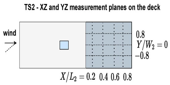
Figure 9.
TS2 measurement planes.
Figure 10a presents the vertical wind profile of the time-averaged velocity magnitude at across four streamwise positions in the ROI for subcase 1, where the inlet reference wind velocity is set to 4.8 m/s from the west (270 degrees). For this case, QUIC reproduces the wind tunnel trends with close agreement, exhibiting only minor deviations in the near-wake region ( and ) and modest over predictions in the far wake, particularly above the deck height. In contrast, subcase 2, which corresponds to a higher inflow velocity of 12 m/s from the same direction (270 degrees, see Figure 10b), shows significant under predictions of velocity at all downstream positions. These findings suggest that QUIC’s predictive performance deteriorates as inflow wind speed increases.
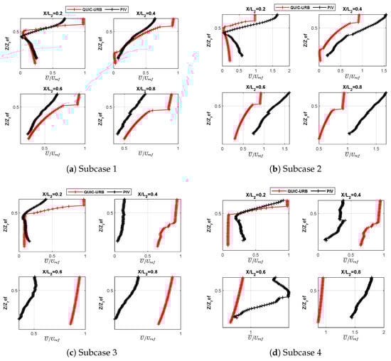
Figure 10.
TS2-Wind tunnel measurements vs. QUIC-URB velocity magnitude comparison at in the XZ plane.
For subcase 3 (4.8 m/s at 240 degrees, Figure 10c), where the inflow wind direction is varied, QUIC over predicts the velocity magnitude across all downstream positions. The only exception occurs in the near-wake region (), where QUIC initially follows the wind tunnel profile up to the deck height, beyond which it consistently overestimates the velocity, whereas in subcase 4 (12 m/s at 240 degrees, Figure 10d), the velocity magnitude is under predicted. A behavior similar to that of subcase 2 but more pronounced. While subcase 2 qualitatively preserves the shape of the wind tunnel trend, albeit with lower magnitudes, subcase 4 departs more substantially, not only in magnitude but also in the structure of the vertical profiles across the four streamwise positions. On the whole, these results indicate that QUIC exhibits systematic biases and potential limitations in how the solver parametrizes flow regions or represents wake geometry for higher inflow wind velocity and oblique wind approach angles.
Figure 11 provides a visual representation of the overall flow field, illustrating the velocity magnitude and streamlines for subcases 1 and 3 at to enable a qualitative assessment of the wake structures. The wind tunnel data (see Figure 11a) show a pronounced recirculation zone behind the building, characterized by swirling streamlines and an extended region of low velocity. The QUIC solver also predicts the rear wake, but it appears smaller in size and less defined. It can be noticed that the reattachment lengths of the wake are approximately the same; however, it is evident that the vortex core in the wind tunnel data are located farther downstream from the deck structure, whereas in the QUIC results, the vortex core is positioned much closer to the structure.
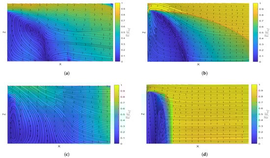
Figure 11.
TS2-Steady state velocity magnitude, and streamlines of flow field at or port side XZ plane on the Ship deck (ROI). (a) Subcase 1-PIV measurements (Ref. [33]). (b) Subcase 1-QUIC-URB. (c) Subcase 3-PIV measurements (Ref. [33]). (d) Subcase 3-QUIC-URB.
Contrary to subcase 1, the QUIC solver in subcase 3 fails to capture the recirculation zone, with streamlines largely following the contours of the deck structure and exhibiting minimal rotation. The velocity contours further reveal higher velocities in this region compared to the wind tunnel data, where a distinct vortex develops closer to the deck structure, with its core located near the base, along with an extended region of low velocity downstream. Although QUIC does indicate the formation of a vortex near the structure, it is considerably less pronounced than in the wind tunnel data and positioned farther laterally at . This discrepancy provides a direct visual explanation for the significant velocity over predictions observed in Figure 10c, reinforcing QUIC’s inability to capture lateral flow variations and to reproduce the low-speed reverse flow region under inclined wind approach angles that constitutes a fundamental component of the wake structure. Notably, these steady-state computations required only 25 s using QUIC.
3.2.3. TS3 Multi-Building Results Analysis
In this section, validation is carried out using a published dataset [44]. The dataset supports the study presented in [34,35], which focuses on Large Eddy Simulations (LES) of an array of staggered buildings. The analysis points and ROI for TS3 are shown in Figure 12.
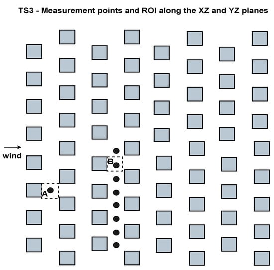
Figure 12.
TS3 measurement points (black dots) placed at 10 m (laterally and longitudinally) from the obstacle to cover critical flow regions.
Figure 13 presents the streamwise and lateral variations in the time-averaged steady-state velocity vectors for the four repeating units at half of (the mean building height across the staggered array), alongside the vertical velocity variations downstream of row 3 indicated by the black line in Figure 13a,b. QUIC-URB produces a more symmetric and smoother depiction of the upwind, lateral, and lee-side wake structures, whereas the LES results reveal a more localized and heterogeneous flow pattern. Notably, LES captures lateral flow meanderings induced by taller upstream buildings. For instance, between the buildings with heights of 10 mm and 13.6 mm in the first row, LES shows enhanced acceleration on the side of the taller building (13.6 mm), which in turn influences the downstream flow and vortex structures, as observed in the upwind wake region of row 2. Similarly, the accelerated lateral flow around the 17.2 mm building in row 3 persists further downstream, modifying the flow characteristics in the vicinity of downstream structures. These asymmetric lateral deviations are substantially less pronounced in the QUIC-URB results, where the flow within building gaps or along building sides primarily aligns with the inflow wind direction (top to bottom), thereby approximating the actual complexity of the flow. Although QUIC-URB does capture accelerated flow around taller buildings, the magnitude of these accelerations is generally lower than in LES.
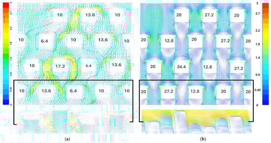
Figure 13.
Averaged steady state velocity magnitude vectors, , at and over the 4 ‘repeating units’ in the TS3 domain (inflow wind is from the top to the bottom). Note: White squares indicate buildings, with numbers inside representing building heights. In (b), buildings are shown at a 2000× upscaled size (in meters), whereas in (a), buildings are depicted at a millimeter scale. (a) LES vectors (image from [35]). (b) Vectors as simulated by QUIC-URB.
From the LES and QUIC-URB vertical planes of the flow behind row 3, it is evident that LES resolves coherent recirculation zones within the gaps between buildings. For example, the vortex on the right side of the taller building rotates in an anti-clockwise direction, while the vortex on the left rotates clockwise. In contrast, QUIC-URB predicts both recirculations to be anti-clockwise. QUIC also estimates the vertical velocity magnitudes above the rooftops to be consistently greater than 2.2 m/s. This feature, however, is not observed in LES.
The mean velocity magnitude of the vertical wind profiles from wind tunnel measurements, LES, and QUIC at eight lateral positions downstream of row 3 (, see Figure 12) are qualitatively compared in Figure 14. Overall, QUIC exhibits a systematic positive bias, consistently over predicting the velocity magnitudes, whereas LES shows excellent agreement with the experimental measurements. Notably, QUIC predicts prominent recirculation regions at , 3, and 4, despite these lateral positions being the side and lee zones of the shortest building in the row. This behavior corroborates the observation made in Figure 13, where QUIC is identified to produce symmetric wake structures across the simulation domain. Albeit such limitations, QUIC captures salient flow features, such as the strong shear at caused by the taller building upstream. Collectively, these findings suggest that QUIC is capable of reproducing the overall flow tendencies and structural patterns in urban-like environments, but with relatively less accuracy.
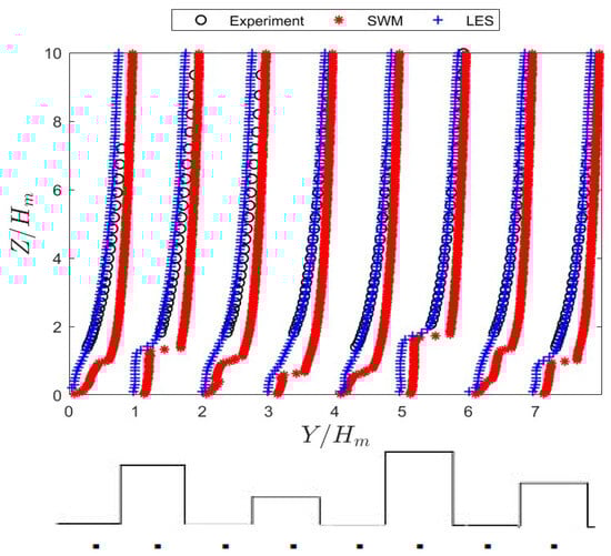
Figure 14.
Mean velocity profile behind column 3 in the repeating unit or at (see dots in Figure 12).
The RMS of the spatially averaged streamwise and vertical velocity components ( and ) at ROI A and ROI B obtained from the SWM simulations are compared in Figure 15 with wind tunnel measurements and LES data. In both ROIs, the LES results exhibit two distinct peaks at and , corresponding to the shedding of shear layers generated by the upstream building of height m. The experimental data also indicate similar trends, though with slight variations in magnitude between ROI A and ROI B. In contrast, the SWM results show nearly identical magnitudes and profiles at both ROIs. For , the SWM simulations capture the peaks at and , but with significantly higher magnitudes compared to LES and experimental results. Furthermore, SWM predicts an additional peak at , which is not observed in LES or experiments and cannot be attributed to any upstream building feature. For , the SWM results show weaker shear-layer shedding compared to LES and experimental data, and at , the vertical velocity fluctuations fail to decay and instead increase, which is inconsistent with physical expectations. Another key difference is that the SWM results exhibit larger noise levels than LES and experimental data, a characteristic typical of stochastic turbulence generators, where random fluctuations are superimposed on the inflow mean wind profile. At first glance, this may suggest that SWM fails to reproduce realistic turbulence structures or intensities. However, closer inspection reveals that SWM is still able to capture shear-layer formation at approximately the same heights as LES, albeit with misestimated magnitudes.
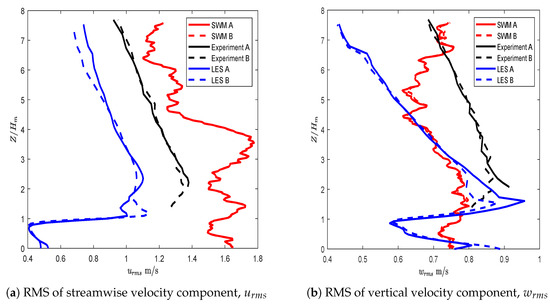
Figure 15.
Spatially averaged velocity RMS at ROI A and ROI B (see Figure 12).
The total computation time for TS3 is roughly 1 and a half hours, with around 250 s for the steady-state simulation and approximately 100–120 s for turbulence generation for a single YZ plane within an ROI.
4. WRF–SWM Integrated Simulation
Wind speed, TI, and directional variability are critical factors influencing vertiport safety, capacity, and UAM aircraft performance during take-off, landing, and transition phases. This necessitates a detailed understanding of the local wind environment surrounding the Vertiport infrastructure to evaluate operational feasibility and anticipate site-specific deviations in UAM aircraft performance. Therefore, in this section, the SWM is integrated with the mesoscale WRF model to establish the WRF-SWM framework, illustrated via its application to a potential vertiport site in Milan, Italy.
4.1. Potential Vertiport Site Identification
The selection of a potential vertiport location in Milan aims to support the broader objective of integrating UAM within the existing urban infrastructure and mobility systems—an approach implied in the Single European Sky Air traffic management research (SESAR), EASA’s U-space ConOps [45], and potentially applicable within the framework of Milan’s Sustainable Urban Mobility Plan (SUMP) [46,47]. Building on this context, and following the findings of Coppola et al. [48], which suggest that launching UAM services from airports enhances their market appeal, the area surrounding Milan Linate Airport is identified as a promising site for vertiport development. This site also presents a strong opportunity for metro-rail-airport integration, given the recent proposal for extension of the M4 metro line from Milan Linate Airport to Segrate and the “East Gate Hub” project near the Segrate Inter-modal Freight Exchange, which includes the replacement of the existing Segrate railway stop with a new High-Speed Rail (HSR) station [49,50].
The specific site or ROI proposed for the vertiport is the rooftop of the structure located at the rear of Milan Linate Airport, as shown in Figure 16. This region has been strategically selected due to its proximity to key inter-modal elements—the M4 metro station, adjacent parking structures as well as its alignment with the broader redevelopment project. Furthermore, the ROI lies outside the operational runways of the airport, while enabling direct access to both the metro and the airport terminal. As a result, the vertiport can serve a broad user base—i.e., not limited to business aviation–thereby enabling more inclusive UAM service models and enhancing integration with the wider urban mobility ecosystem.
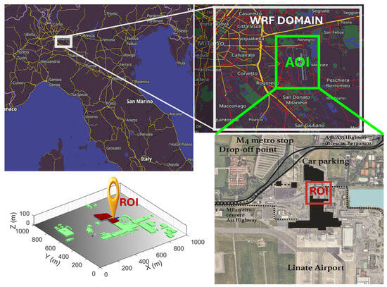
Figure 16.
Map showing the AOI and the potential vertiport site (ROI) near the Milan Linate Airport situated within the WRF domain.
4.2. WRF-SWM Integration and Simulation Setup
The WRF model is a state-of-the-art, open-source numerical weather prediction system that offers advanced physics parameterizations and the flexibility to be configured for either real-case forecasting or idealized research experiments [51]. Within the SWM framework, the QUIC solver provides a straightforward one-way coupling with WRF, where mesoscale outputs from WRF are used to define boundary conditions for QUIC’s microscale steady-state simulations [52]. For this study, a single WRF domain of 20 km × 20 km centered on the Linate Airport in Milan is configured with a horizontal grid resolution of 200 m (see Figure 16). The vertical discretization consists of 34 layers, extending from the ground to 1000 m altitude. The simulation is performed for a 3 h period on 28 August 2025, from 00 h to 03 h UTC. The boundary conditions are derived from the NCEP operational Global Forecast System (GFS) analysis and forecast data [53] while the topography information is taken from the default WRF dataset. The physics configuration follows the setup in [51], where the Bougeault Lacarrère planetary boundary layer scheme, the Noah land surface model, and the ETA surface layer scheme are used to capture the boundary layer processes along with the land–atmosphere interactions. To optimize computational efficiency, memory usage to execute the WRF simulation on a standard laptop, other physics options—such as cumulus and urban canopy models—are disabled. For more details on the physics options and WRF modeling, the readers are referred to [54,55,56,57].
The QUIC domain or AOI spans 1 km × 1 km × 100 m. It is centered on the ROI and nested within the WRF domain. A grid resolution of 1 m is employed, resulting in a total of 100 million cells. Building information within the domain is sourced from the open-access platform OpenStreetMap [58]. Boundary conditions are defined by importing the WRF NetCDF output at 00h into QUIC (multiple forecast hour outputs can also be used). QUIC then automatically pre-processes and interpolates the necessary input parameters—including wind speed, wind direction, temperature, pressure, and skin friction velocity—based on the QUIC domain’s position within the WRF extent to enable the steady-state wind simulation.
For the unsteady wind generation, a total of 67 YZ TurbSim planes are arranged horizontally with a 1 m spacing along the X-direction above the rooftop of the building or ROI. Each plane measures 75 × 100 m with a 1 m grid resolution. Given that the ROI height H is approximately 18m, the TI is set to a median value of 10%, consistent with the observations of [59] for rooftop flows over low-rise buildings. The reference wind speed, 3.5 m/s with 90° direction, is extracted from the WRF output at 100 m altitude above ground level. The coherence model, associated parameters, and turbulence spectrum are the same as those specified for the test scenarios in Table 2.
4.3. Simulated Wind Conditions Around the Proposed Vertiport Site
This section aims to provide a preliminary understanding of wind flow conditions across the ROI or Vertiport site using data from the WRF–SWM simulation. For simplicity, instead of analyzing 4D wind data across the entire ROI—which is substantial—only selected planes are examined (see Figure 17a). Specifically, 15 planes are analyzed along the X-axis and 16 planes along the Y-axis, with a 3 m spacing between adjacent planes in both directions.
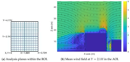
Figure 17.
Rooftop ROI analysis planes and simulated steady-state wind velocity field with streamlines around the proposed vertiport site.
Figure 17b presents the streamlines and time-averaged velocity magnitude field within the ROI. It can be observed that as the approaching wind encounters the sharp leading edge of the roof, the flow separates, generating a recirculation zone that extends approximately 3.5 m vertically and 26 m (or ) downstream. Within this reverse flow region, the mean velocity remains relatively low (<3 m/s) compared to the area immediately above the rooftop recirculation zone, where the flow accelerates to nearly 6 m/s. Additionally, the figure also highlights the building’s influence on the ABL, as the accelerated flow above the recirculation region persists up to nearly 50 m (or approximately 3H) beyond the rooftop height.
Figure 18 illustrates the simulated non-stationary turbulent velocity field and distribution of TI across the X-, Y-, and Z-direction on the rooftop. The highest TI values occur near the shear layer above the rooftop edge and in the recirculation region at 1 to 2 and , where the accelerated flow interacts with the vortex. Above , the TI decreases rapidly, and the flow can be seen becoming more uniform, indicating a diminishing influence of building-induced flow changes. Along similar lines, lateral TI distribution indicates localized peaks near the roof side-corners, suggesting the secondary shear zones caused by the nearby buildings.
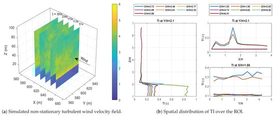
Figure 18.
Spatial and temporal distribution of turbulent wind velocity and TI across the ROI.
Overall, these observations suggest the presence of unsteady wind flow and gusts within the first 30 to 40 m above the rooftop surface—precisely where the FATO would be located if this area were to be used as a vertiport. The findings can also help identify rooftop zones to avoid, such as regions directly above recirculation or shear layers, and highlight areas with lower TI that minimize exposure to the turbulent rooftop wake.
The total computation time for the WRF-SWM integrated simulation was approximately 6 h, with WRF accounting for the majority of the time (approximately 4 hrs), while QUIC required roughly 550 s and TurbSim took about 150–180 s to simulate a plane within the ROI.
5. Conclusions and Recommendations for Future Research
This article outlines the process of developing a novel Stochastic Microscale Wind Modeling framework, SWM, for UAM applications and evaluates its performance by replicating three carefully chosen wind tunnel test scenarios—TS1, TS2, and TS3—with varying levels of complexity. The comparative assessment delineates the strengths and methodological limitations of the proposed stochastic wind modeling approach by evaluating the performance of the constituent steady state solver, QUIC-URB, and the inflow turbulence generator, TurbSim, within the context of UAM applications. The key insights derived from this validation effort are summarized in the list below.
- 1.
- In all test cases, QUIC consistently captured the fundamental mean flow patterns around buildings or obstacles within the domain, including rooftop shear layers, upwind recirculation zones, and wake regions, albeit with an expected degree of inaccuracy. For example, in TS1, the steady-state vertical velocity profiles exhibited strong agreement with experimental measurements, whereas lateral flow profiles showed discrepancies, with velocity magnitudes either over- or under-estimated at increasing heights within the rear wake region. TS2 analysis indicated that the predictive accuracy of QUIC diminishes with increasing inflow wind speeds and oblique inflow angles. Subcases with lower wind speeds showed trends closer to experimental measurements, whereas higher wind speed scenarios exhibited significant over-prediction. Likewise, subcases with a 270° wind approach angle showed better agreement, while those with a 240° approach angle were under-predicted. Lateral flow disparities, consistent with those observed in TS1 and TS3, were also present. In TS3, QUIC captured the overall flow topology; however, the solution was overly smooth with excessive symmetry. That is, the solver was unable to resolve the complex interactions between the upstream and downstream flows around buildings of varying heights, producing minimal to no lateral flow variations.
- 2.
- Validation of the TS1 and TS3 unsteady wind flow fields shows that TurbSim can generate wind velocity magnitudes roughly comparable with experimental measurements. However, this can be achieved only when key parameters—such as time step size (with smaller steps improving accuracy), TI at the reference height, and coherence settings—are carefully tuned. Despite these input parameter adjustments, the synthesized turbulence still fails to reproduce the coherent structures and localized flow patterns that naturally develop behind buildings, highlighting the inherent limitations of TurbSim in representing urban microscale turbulence.
- 3.
- Notwithstanding the limitations, SWM maintains relatively good computational efficiency. Steady-state simulations with QUIC typically complete in under 10 min, while TurbSim-based unsteady realizations require less than 2 h. This provides a substantial reduction in computational cost while achieving a balanced trade-off between efficiency and accuracy compared with high-fidelity CFD or LES.
A key limitation of the unsteady component prediction in SWM lies in its application of a single TI and coherence model across the entire ROI. In reality, both TI and coherence exhibit strong spatial and temporal variability in urban environments, particularly within recirculation zones, shear layers, and wake regions. This simplification, coupled with the use of IEC-standardized spectra (Kaimal) and coherence functions originally developed for ABL flows over open terrain, constrains TurbSim’s ability to represent wake-specific turbulence structures. Utilizing QUIC-URB-derived mean wind profiles as TurbSim inputs within the SWM framework partially alleviates this issue by embedding spatial variations in mean velocity and shear, which enhances the magnitude of the synthesized fluctuations. However, the resulting turbulence fields still lack the distinct anisotropy and localized coherent structures—such as shear-layer roll up and vortex shedding—commonly observed in experimental or CFD studies of flow across urban areas. Accurate reproduction of these features would require high-resolution, spatially resolved TI and coherence data from field sensors, wind tunnel measurements, or Direct Numerical Simulations (DNSs). Unfortunately, acquiring such data are inherently challenging—both practically and financially as urban turbulence exhibits multi-factor dependence along with strong spatio-temporal variability. Moreover, the difficulty in predicting these wake structures is not simply an implementation issue; it reflects a broader, fundamental challenge in turbulence research, as the turbulent transport and coherent-structure predictability remain open and hard problems even for high-fidelity CFD [60,61]. Overall, although SWM does not dynamically resolve turbulence evolution in the same first-principles sense as DNS or LES, its composite output (QUIC mean + stitched TurbSim fluctuations) produces a spatio-temporally varying—i.e., quasi-non-stationary—field that captures essential variability at lower computational cost. This, for many UAM and vertiport safety studies focusing on initial UAM aircraft controller design, performance evaluation, vertiport emplacements, and simulation-based flight testing, such as these research efforts [62,63,64,65,66,67,68,69,70,71], is an application-driven trade-off. SWM’s flexibility to integrate with mesoscale models like WRF via QUIC paves the way for preliminary cost-effective simulation-based operational area-specific UAM aircraft risk assessment to support flight testing for certification, Vertiport emplacements, and design. Furthermore, the efficiency and modular design of SWM enable its potential integration with machine learning and deep learning–based urban microscale wind forecasters—such as those explored in [72,73,74,75]—by allowing the rapid generation of large ensembles of synthetic microscale wind fields under varied input conditions. However, given SWM’s current limitations, such integration should be pursued cautiously until further refinements ensure a reliable representation of urban wind fields.
Future work to refine SWM should begin with analysis of the spectral characteristics of turbulence in key flow regions within the urban canopy using sensor measurements, wind tunnel tests, or high-fidelity CFD simulation data. Such analysis would improve the understanding of the spatio-temporal variations in velocity fluctuations by revealing correlations between turbulence spectra and factors such as inflow wind speed, direction, and static parameters like building dimensions and geometry. Additionally, spatial/temporal coherence and correlation analyses should also be conducted to predict coherent turbulent structures with reasonable accuracy [76,77]. The resulting data can be compiled into databases or look-up tables to approximate turbulence characteristics within the ROI, providing improved inputs for TurbSim simulations and the generation of unsteady turbulence fields. Additionally, TurbSim’s performance in generating turbulence is directly dependent on the accuracy of QUIC-URB predictions. That is, errors in the mean wind flow propagate into the synthesized fluctuations. Therefore, addressing current SWM limitations also requires refinements to the steady-state solver, QUIC-URB. These alterations should focus on improving the prediction of lateral flow variations and flow regions for high inflow speeds or oblique approach angles to better capture the complex urban flow phenomena. Finally, uncertainty analysis should be performed to rigorously quantify the accuracy or bounds of SWM prediction variability by assessing how differences between SWM-generated and experimentally measured wind velocity and TI fields affect UAM vehicle stability. This would provide a solid foundation for applying SWM in UAM safety assessments and operational risk evaluations.
Author Contributions
Conceptualization, D.S.N., F.M., V.M. and G.Q.; methodology, software, formal analysis, writing—original draft preparation, D.S.N. and F.M.; writing—review and editing, G.Q. and V.M.; supervision, G.Q., M.L. and V.M.; funding acquisition, G.Q. and V.M. All authors have read and agreed to the published version of the manuscript.
Funding
This research is conducted under the REDI (RMIT European Doctoral Innovators) Program. This project has received funding from the European Union’s Horizon 2020 research and innovation programme under the Marie Skłodowska-Curie grant agreement no. 101034328.
Data Availability Statement
The data are available upon request from the corresponding author.
Acknowledgments
The authors would like to thank the QUIC-URB team at the Los Alamos National Laboratory, USA, and the management staff at the Department of Aerospace Science and Technology in Politecnico di Milano, Italy, for providing and obtaining the QUIC software (version 6.4.8) license, respectively.
Conflicts of Interest
The authors declare no conflicts of interest. Results reflect the authors’ view only. The European Union had no role in the design of the study; in the collection, analysis, or interpretation of data; in the writing of the manuscript; or in the decision to publish the results. The Research Executive Agency is not responsible for any use that may be made of the information the article contains.
Abbreviations
The following abbreviations are used in this manuscript:
| ABL | Atmospheric Boundary Layer |
| AD | Atmospheric Disturbance |
| AOI | Area Of Interest |
| CFD | Computational Fluid Dynamics |
| ConOps | Concept of Operations |
| DNS | Direct Numerical Simulation |
| EASA | European Aviation Safety Agency |
| eVTOLs | Electric Vertical Take-Off and Landing Aircraft |
| FATO | Final Approach and Take-Off area |
| IEC | International Electrotechnical Commission |
| LES | Large Eddy Simulation |
| MRE | Mean Relative Error |
| NCEP | National Centers for Environment Prediction |
| NetCDF | NETwork Common Dataform |
| PIV | Particle Image Velocimetry |
| QES | Quick Environmental Simulation |
| QUIC-URB (or) QUIC | Quick Urban and Industrial Complex - URBan |
| RAM | Random Access Memory |
| RMSE | Root Mean Square Error |
| RMS | Root Mean Square |
| ROI | Region(s) of Interest |
| RPAs | Remotely Piloted Aircraft |
| SWM | Stochastic Microscale Wind Model |
| TI | Turbulence Intensity |
| TS | Test Scenario |
| UAM | Urban Air Mobility |
| UAVs | Uncrewed Aerial Vehicles |
| UBL | Urban Boundary Layer |
| VTOL | Vertical Take-Off and Landing aircraft |
| WRF | Weather Research and Forecasting |
References
- Global Industry Analysts, Inc. eVTOL Aircrafts-Global Strategic Business Report. Research and Markets Report, 2024. Available online: https://www.researchandmarkets.com/reports/5997780/evtol-aircrafts-global-market-report. (accessed on 1 December 2025).
- Federal Aviation Administration. Urban Air Mobility (UAM) Concept of Operations v2.0; Technical Report; Federal Aviation Administration (FAA): Washington, DC, USA, 2023. Available online: https://www.faa.gov/air-taxis/uam_blueprint (accessed on 1 December 2025).
- Gregory, I.M. Urban Air Mobility: A Control-Centric Approach to Addressing Technical Challenges. In Presentation NTRS Document ID: 20210015453, National Aeronautics and Space Administration; Langley Research Center: Hampton, VA, USA, 2021. [Google Scholar]
- Connors, M.M. Understanding Risk in Urban Air Mobility: Moving Towards Safe Operating Standards; NASA Technical Memorandum NASA/TM–20205000604; NASA Ames Research Center: Moffett Field, CA, USA, 2020. Available online: https://ntrs.nasa.gov/citations/20205000604 (accessed on 1 December 2025).
- Hamilton, B.A. Urban Air Mobility (UAM) Market Study-Final Report. In Final Report NASA NTRS Document ID: 20190001472; NASA Aeronautics Research Mission Directorate: Washington, DC, USA, 2018. Available online: https://ntrs.nasa.gov/api/citations/20190001472/downloads/20190001472.pdf (accessed on 1 December 2025).
- Hill, B.P.; DeCarme, D.; Metcalfe, M.; Griffin, C.; Wiggins, S.; Metts, C.; Bastedo, B.; Patterson, M.D.; Mendonca, N.L. UAM Vision Concept of Operations (ConOps) UAM Maturity Level (UML) 4; Technical Report NASA NTRS Document ID: 20205011091; NASA Aeronautics Research Mission Directorate: Washington, DC, USA, 2020. [Google Scholar]
- European Union Aviation Safety Agency (EASA). Prototype Technical Specifications for the Design of VFR Vertiports for Operation with Manned VTOL-Capable Aircraft Certified in the Enhanced Category (PTS-VPT-DSN); Technical Report; European Union Aviation Safety Agency: Cologne, Germany, 2024; Available online: https://www.easa.europa.eu/en/document-library/general-publications/prototype-technical-design-specifications-vertiports (accessed on 1 December 2025).
- Federal Aviation Administration (FAA); Airport Engineering Division. Engineering Brief No. 105, Vertiport Design; Engineering Brief EB-105; Federal Aviation Administration: Washington, DC, USA, 2022; Available online: https://acconline.org/wp-content/uploads/Engineering-Brief-105-1.pdf (accessed on 1 December 2025).
- Federal Aviation Administration (FAA). Flight Operational Quality Assurance (FOQA)-Advisory Circular AC 120-82; Advisory Circular AC 120-82; Federal Aviation Administration: Washington, DC, USA, 2004. Available online: https://www.faa.gov/documentLibrary/media/Advisory_Circular/AC_120-82.pdf (accessed on 1 December 2025).
- European Union Aviation Safety Agency (EASA). Means of Compliance with the Special Condition VTOL (MOC SC-VTOL); Issue 2. Technical Report; European Union Aviation Safety Agency: Cologne, Germany, 2023; Available online: https://www.easa.europa.eu/sites/default/files/dfu/MOC-3_SC-VTOL_-_Issue_2_-_21_Jun_2023_-_FINAL.pdf (accessed on 1 December 2025).
- Anderson, J.D. Aircraft Performance and Design, 1st ed.; McGraw-Hill: New York, NY, USA, 1999. [Google Scholar]
- Cook, M.V. Flight Dynamics Principles: A Linear Systems Approach to Aircraft Stability and Control, 3rd ed.; Butterworth-Heinemann: Oxford, UK, 2013. [Google Scholar]
- Nithya, D.S.; Quaranta, G.; Muscarello, V.; Liang, M. Review of Wind Flow Modelling in Urban Environments to Support the Development of Urban Air Mobility. Drones 2024, 8, 123. [Google Scholar] [CrossRef]
- Giersch, S.; Guernaoui, O.E.; Raasch, S.; Sauer, M.; Palomar, M. Atmospheric flow simulation strategies to assess turbulent wind conditions for safe drone operations in urban environments. J. Wind. Eng. Ind. Aerodyn. 2022, 229, 105136. [Google Scholar] [CrossRef]
- Kaimal, J.C.; Finnigan, J.J. Atmospheric Boundary Layer Flows: Their Structure and Measurement, 1st ed.; Oxford University Press: New York, NY, USA, 1994. [Google Scholar]
- Pinus, N.Z. Low-Level Atmospheric Turbulence Affecting Aircraft Flight; Technical Report; Trudy (Central Aerological Observatory): Moscow, Russia, 1967. [Google Scholar]
- Pope, S.B. Turbulent Flows, 1st ed.; Cambridge University Press: Cambridge, UK, 2000. [Google Scholar]
- Stull, R.B. An Introduction to Boundary Layer Meteorology, 1st ed.; Atmospheric and Oceanographic Sciences Library, Springer: Dordrecht, The Netherlands, 1988; Volume 13. [Google Scholar]
- Nelson, M.; Brown, M. The QUIC Start Guide v6.01: The Quick Urban and Industrial Complex (QUIC-URB) Dispersion Modeling System; Technical Report; Los Alamos National Laboratory: Los Alamos, NM, USA, 2013. Available online: https://cdn.lanl.gov/files/quic-startguide_7c182.pdf (accessed on 1 December 2025).
- Kelley, N.D.; Jonkman, B.J. Overview of the TurbSim Stochastic Inflow Turbulence Simulator; Technical Report NREL/TP-500-39796; Version 1.10; National Renewable Energy Laboratory (NREL): Golden, CO, USA, 2006; Available online: https://digital.library.unt.edu/ark:/67531/metadc886250/ (accessed on 1 December 2025).
- Rökle, R. Bestimmung der Strömungsverhältnisse im Bereich Komplexer Bebauungsstrukturen. Ph.D. Thesis, Technische Hochschule Darmstadt, Darmstadt, Germany, 1990. Available online: https://www.deutsche-digitale-bibliothek.de/item/LRKWIGQI4A37AMOLZQDIBS3BQOU32CTU (accessed on 1 December 2025).
- Brown, M.J.; Williams, M.D.; Nelson, M.A.; Werley, K.A. QUIC transport and dispersion modeling of vehicle emissions in cities for better public health assessments. Environ. Health Insights 2015, 9, 1–11. [Google Scholar] [CrossRef] [PubMed]
- Singh, B.; Hansen, B.S.; Brown, M.J.; Pardyjak, E.R. Evaluation of the QUIC-URB fast response urban wind model for a cubical building array and wide building street canyon. Environ. Fluid Mech. 2008, 8, 521–540. [Google Scholar] [CrossRef]
- Pardyjak, E.R.; Brown, M.J. Evaluation of a Fast-Response Urban Wind Model—Comparison to Single-Building Wind Tunnel Data; Technical Report LA-UR-01-4028. Los Alamos National Laboratory: Los Alamos, NM, USA, 2001. Available online: https://digital.library.unt.edu/ark:/67531/metadc718282/ (accessed on 1 December 2025).
- Gowardhan, A.A.; Brown, M.J.; Williams, M.D.; Pardyjak, E.R. Evaluation of the QUIC Urban Dispersion Model using the Salt Lake City URBAN 2000 Tracer Experiment Data—IOP 10. In Proceedings of the 6th Symposium on the Urban Environment, 86th AMS Annual Meeting, Atlanta, GA, USA, 29 January–2 February 2006; Los Alamos National Laboratory Report LA-UR-05-9017. Available online: https://ams.confex.com/ams/pdfpapers/104237.pdf (accessed on 1 December 2025).
- Jonkman, J.E.; Butterfield, S.; Musial, W.; Scott, G. TurbSim User’s Guide v2.00.00; National Renewable Energy Laboratory (NREL): Golden, CO, USA, 2006. Available online: https://www.nrel.gov/docs/libraries/wind-docs/turbsim_v2-00-pdf.pdf (accessed on 1 December 2025).
- Nithya, D.S.; Quaranta, G.; Muscarello, V.; Liang, M. Assessment of a Highly Parameterized Steady-State Microscale Wind Simulator for Urban Air Mobility Applications. In Proceedings of the 34th International Congress of the Aeronautical Sciences (ICAS 2024), Florence, Italy, 9–13 September 2024; Available online: https://www.icas.org/ICAS_ARCHIVE/ICAS2024/data/papers/ICAS2024_0379_paper.pdf (accessed on 1 December 2025).
- Civil Aviation Safety Authority (CASA). ADVISORY CIRCULAR AC 139.V-01 v1.0: Guidance for Vertiport Design; Civil Aviation Safety Authority: Canberra, Australia, 2023. Available online: https://www.casa.gov.au/sites/default/files/2023-07/advisory-circular-139.v-01-guidance-vertiport-design.pdf (accessed on 1 December 2025).
- Johnson, M. High-Density Automated Vertiport Concept of Operations; Technical Report NASA/CR-20210010603; National Aeronautics and Space Administration (NASA): Washington, DC, USA, 2021. Available online: https://ntrs.nasa.gov/api/citations/20210010603/downloads/20210010603_MJohnson_VertiportAtmtnConOpsRprt_final.pdf (accessed on 1 December 2025).
- Utah Environmental Fluid Dynamics (UtahEFD) Group. UtahEFD/QES-Public: Quick Environmental Simulation (QES) for Urban Wind and Dispersion Modeling; Zenodo/GitHub: Salt Lake City, UT, USA, 2024; Version 2.2.0; Available online: https://github.com/UtahEFD/QES-Public (accessed on 1 December 2025).
- Bozorgmehr, B.; Willemsen, P.; Margairaz, F.; Gibbs, J.A.; Patterson, Z.; Stoll, R.; Pardyjak, E.R. QES-Winds v2.2.0: Theory and User’s Guide; University of Utah/Zenodo: Salt Lake City, UT, USA, 2024. [Google Scholar] [CrossRef]
- Meng, Y.; Hibi, K. Turbulent measurements of the flow field around a high-rise building. J. Wind. Eng. 1998, 76, 55–64. [Google Scholar] [CrossRef]
- Taymourtash, N. Experimental Investigation of Helicopter-Ship Dynamic Interface. Ph.D. Thesis, Politecnico di Milano, Milan, Italy, 2022. Available online: https://hdl.handle.net/20.500.14242/207136 (accessed on 1 December 2025).
- Cheng, H.; Castro, I.P. Near Wall Flow Over Urban-Like Roughness. Bound.-Layer Meteorol. 2002, 104, 229–259. [Google Scholar] [CrossRef]
- Xie, Z.T.; Coceal, O.; Castro, I.P. Large-Eddy Simulation of Flows over Random Urban-like Obstacles. Bound.-Layer Meteorol. 2008, 129, 1–23. [Google Scholar] [CrossRef]
- Zou, J.; Yu, Y.; Liu, J.; Niu, J.; Chauhan, K.; Lei, C. Field measurement of the urban pedestrian level wind turbulence. Build. Environ. 2021, 194, 107713. [Google Scholar] [CrossRef]
- U.S. Department of Defense. Flying Qualities of Piloted Aircraft; Military Standard MIL-STD-1797A; U.S. Department of Defense: Arlington County, VA, USA, 1982. [Google Scholar]
- International Electrotechnical Commission (IEC). IEC 61400-1:2019-Wind Energy Generation Systems—Part 1: Design Requirements. Standard IEC 61400-1:2019; International Electrotechnical Commission: London, UK, 2019. Available online: https://webstore.iec.ch/en/publication/26423 (accessed on 1 December 2025).
- Smith, O.E.; Adelfang, S.I. A Compendium of Wind Statistics and Models for the NASA Space Shuttle and Other Aerospace Vehicle Programs; Technical Report NASA/CR-1998-208859; NASA Marshall Space Flight Center: Madison County, AL, USA, 1998. Available online: https://ntrs.nasa.gov/citations/19990008476 (accessed on 1 December 2025).
- Barlow, J.F.; Coceal, O. A Review of Urban Roughness Sublayer Turbulence; Technical Report 527; Met Office: Exeter, UK, 2009; Available online: https://centaur.reading.ac.uk/38572/1/2009BarlowCocealMETOFF_reviewurbRSL.pdf (accessed on 1 December 2025).
- Bernard, J.; Lindberg, F.; Oswald, S. URock 2023a: An open-source GIS-based wind model for complex urban settings. Geosci. Model Dev. 2023, 16, 5703–5724. [Google Scholar] [CrossRef]
- Hansen, A.C.; Peterka, J.A.; Cermak, J.E. Wind-Tunnel Measurements in the Wake of a Simple Structure in a Simulated Atmospheric Flow. Contractor Report NASA-CR-2540; NASA: Washington, DC, USA, 1975. Available online: https://ntrs.nasa.gov/citations/19750012586/downloads/19750012586.pdf (accessed on 1 December 2025).
- Woo, H.G.C.; Peterka, J.A.; Cermak, J.E. Wind Tunnel Measurements in the Wakes of Structures; Contractor Report NASA-CR-2806; NASA: Washington, DC, USA, 1977. Available online: https://ntrs.nasa.gov/api/citations/19770012772/downloads/19770012772.pdf (accessed on 1 December 2025).
- Xie, Z.T.; Coceal, O.; Castro, I.P. Dataset for Large-Eddy Simulation of Flows over Random Urban-Like Obstacles; Institutional Repository; University of Southampton: Hampshire, UK, 2019. [Google Scholar] [CrossRef]
- SESAR Joint Undertaking. U-Space ConOps and Architecture, 4th ed.; Technical Report; SESAR Joint Undertaking: Brussels, Belgium, 2023; Available online: https://www.sesarju.eu/node/4544 (accessed on 1 December 2025).
- Piano Urbano della Mobilità Sostenibile della Città Metropolitana di Milano: Documento di Piano. Technical Report, Città Metropolitana di Milano, 2021. Available online: https://www.cittametropolitana.mi.it/PUMS/Pums (accessed on 1 December 2025).
- UIC2–UAM Initiative Cities Community, EU’s Smart Cities Marketplace. Urban Air Mobility and Sustainable Urban Mobility Planning–Practitioner Briefing, 2021. Available online: https://urban-mobility-observatory.transport.ec.europa.eu/system/files/2023-11/urban_air_mobility_and_sump.pdf (accessed on 27 November 2025).
- Coppola, P.; Fabiis, F.D.; Silvestri, F. Urban Air Mobility (UAM): Airport shuttles or city-taxis? Transp. Policy 2024, 150, 24–34. [Google Scholar] [CrossRef]
- Giunta Regionale della Lombardia. Delibera N.4962, XII Legislatura: Approvazione dello Schema di Accordo tra Regione Lombardia, Città Metropolitana di Milano, Comune di Milano, Comune di Segrate, Rete Ferroviaria Italiana S.p.A., Con l’Adesione di Westfield Milan S.p.A., per il Coordinamento Degli Interventi Previsti Nell’Ambito Dell’Hub Porta Est (di Concerto Con l’Assessore Lucente). Available online: https://www.regione.lombardia.it/wps/portal/istituzionale/HP/istituzione/Giunta/sedute-delibere-giunta-regionale/DettaglioDelibere/delibera-4962-legislatura-12 (accessed on 1 December 2025).
- Balasubramanian, A. Milan East Gate Hub: An Urbanlink: Multimodal transportation hub in Segrate. Master’s Thesis, Politecnico di Milano, Milan, Italy, 2023. Available online: https://hdl.handle.net/10589/230852 (accessed on 1 December 2025).
- Skamarock, W.C.; Klemp, J.B.; Dudhia, J.; Gill, D.O.; Barker, D.M.; Wang, M.; Powers, J.G. A Description of the Advanced Research WRF Model Version 4; Technical Report NCAR/TN-556+STR; National Center for Atmospheric Research (NCAR): Boulder, CO, USA, 2019; Available online: https://www2.mmm.ucar.edu/wrf/users/docs/technote/v4_technote.pdf (accessed on 1 December 2025).
- Kochanski, A.K.; Pardyjak, E.R.; Stoll, R.; Gowardhan, A.; Brown, M.J.; Steenburgh, W.J. One-Way Coupling of the WRF–QUIC Urban Dispersion Modeling System. J. Appl. Meteorol. Climatol. 2015, 54, 2119–2139. [Google Scholar] [CrossRef]
- National Centers for Environmental Prediction (NCEP), NOAA. NCEP GFS 0.25° Global Forecast Grids Historical Archive (Updated daily). Available online: https://rda.ucar.edu/datasets/ds084.1/ (accessed on 15 September 2025).
- WRF Development Team, NCAR/UCAR. WRF Users’ Guide, Version 4.5; National Center for Atmospheric Research (NCAR): Boulder, CO, USA, 2024; Available online: https://www2.mmm.ucar.edu/wrf/users/docs/user_guide_v4/contents.html (accessed on 1 December 2025).
- Monin, A.S.; Obukhov, A.M. Basic laws of turbulent mixing in the surface layer of the atmosphere. Tr. Geophys. Inst. Akad. Nauk. SSSR 1954, 24, 163–187. [Google Scholar]
- Bougeault, P.; Lacarrère, P. Parameterization of Orography-Induced Turbulence in a Mesobeta–Scale Model. Mon. Weather. Rev. 1989, 117, 1872–1890. [Google Scholar] [CrossRef]
- Tewari, M.; Chen, F.; Wang, W.; Dudhia, J.; LeMone, M.A.; Mitchell, K.; Ek, M.; Gayno, G.; Wegiel, J.; Cuenca, R.H. Implementation and Verification of the Unified NOAH Land Surface Model in the WRF Model. In Proceedings of the 84th American Meteorological Society Annual Meeting—20th Conference on Weather Analysis and Forecasting/16th Conference on Numerical Weather Prediction, Seattle, WA, USA, 11–15 January 2004; Available online: https://ams.confex.com/ams/84Annual/webprogram/Paper69061.html (accessed on 1 December 2025).
- OpenStreetMap contributors. OpenStreetMap. Available online: https://www.openstreetmap.org (accessed on 1 December 2025).
- Morrison, M.J.; Kopp, G.A. Effects of turbulence intensity and scale on surface pressure fluctuations on the roof of a low-rise building in the atmospheric boundary layer. J. Wind. Eng. Ind. Aerodyn. 2018, 183, 140–151. [Google Scholar] [CrossRef]
- Tominaga, Y.; Wang, L.L.; Zhai, Z.J.; Stathopoulos, T. Accuracy of CFD simulations in urban aerodynamics and microclimate: Progress and challenges. Build. Environ. 2023, 243, 110723. [Google Scholar] [CrossRef]
- Paladin, G.; Jensen, M.H.; Vulpiani, A. Predictability. In Turbulence: A Tentative Dictionary; Tabeling, P., Cardoso, O., Eds.; Springer: Boston, MA, USA, 1994; pp. 75–79. [Google Scholar] [CrossRef]
- Nithya, D.S.; Rylko, A.; Muscarello, V.; Liang, M.; Quaranta, G. Effects of Microscale Wind Disturbance on eVTOL Aircraft Performance During Landing. In Proceedings of the 50th European Rotorcraft Forum, Marseille, France, 10–12 September 2024; pp. 1–8. [Google Scholar]
- Nithya, D.S.; Rylko, A.; Muscarello, V.; Liang, M.; Quaranta, G. Sensitivity Analysis of Urban Air Mobility Aircraft Landing Trajectory Deviation to Microscale Wind Disturbances. In Proceedings of the 81st Annual Forum & Technology Display, eVTOL Technical Session, Philadelphia, PA, USA, 20–22 May 2025; pp. 320–328. [Google Scholar] [CrossRef]
- Nithya, D.S.; Rylko, A.; Muscarello, V.; Liang, M.; Quaranta, G. Towards Determining Wind Disturbance Levels for an Urban Air Mobility Aircraft Through Simulation-Based Flight Testing. In Proceedings of the 51st European Rotorcraft Forum, Venice, Italy, 9–12 September 2025; pp. 1–9. [Google Scholar]
- Banerjee, P.; Corbetta, M.; Jarvis, K.; Smalling, K.; Turner, A. Probability of Trajectory Deviation of Unmanned Aerial Vehicle in Presence of Wind. J. Air Transp. 2023, 31, 128–139. [Google Scholar] [CrossRef]
- Vuppala, R.K.S.S.; Krawczyk, Z.; Paul, R.; Kara, K. Modeling Advanced Air Mobility Aircraft in Data-Driven Reduced Order Realistic Urban Winds. Sci. Rep. 2024, 14, 383. [Google Scholar] [CrossRef]
- Krammer, C.; Holzapfel, F. Estimation of Probability of Exceeding SC-VTOL Performance Requirements During Automatic Landing Using Subset Simulation. In Proceedings of the Vertical Flight Society 79th Annual Forum & Technology Display, West Palm Beach, FL, USA, 16–18 May 2023. Paper 80, Modeling and Simulation session. [Google Scholar] [CrossRef]
- Larose, G.L.; Schajnoha, S.; Al Labbad, M. Development of Turbulence Based Design Criteria for Vertiports. In Proceedings of the Vertical Flight Society 80th Annual Forum & Technology Display, Montréal, QC, Canada, 7–9 May 2024. eVTOL technical session. [Google Scholar] [CrossRef]
- Schajnoha, S.; Larose, G.L.; Al-Labbad, M.; Barber, H.; Wall, A. The Safety of Advanced Air Mobility and The Effects of Wind in the Urban Canyon. In Proceedings of the Vertical Flight Society 78th Annual Forum & Technology Display, Fort Worth, TX, USA, 10–12 May 2022. [Google Scholar] [CrossRef]
- Zyadat, Z.; Horri, N.; Innocente, M.; Statheros, T. Observer-Based Optimal Control of a Quadplane with Active Wind Disturbance and Actuator Fault Rejection. Sensors 2023, 23, 1954. [Google Scholar] [CrossRef]
- Pradeep, P.; Chatterji, G.B.; Sridhar, B.; Edholm, K.; Lauderdale, T.A.; Sheth, K.; Lai, C.F.; Erzberger, H. Wind-Optimal Trajectories for Multirotor eVTOL Aircraft on UAM Missions. In Proceedings of the 2020 AIAA Aviation Forum, Online, 15–19 June 2020. [Google Scholar] [CrossRef]
- Waanders, D.; Salins, S.; Rauleder, J.; Smith, M. A Real-Time Reduced-Order Model for the Atmospheric Boundary Layer Including Roughness Sublayer. In Proceedings of the Vertical Flight Society 81st Annual Forum & Technology Display, Virginia Beach, VA, USA, 20–22 May 2025. Modeling & Simulation IV session, Lichten Runner-Up. [Google Scholar] [CrossRef]
- Shah, T.A.; Stanley, M.C.; Warner, J.E. Generative Modeling of Microweather Wind Velocities for Urban Air Mobility. In Proceedings of the IEEE Aerospace Conference, Big Sky, MT, USA, 1–8 March 2025. [Google Scholar] [CrossRef]
- Chrit, M.; Majdi, M. Operational wind and turbulence nowcasting capability for advanced air mobility. Neural Comput. Appl. 2024, 36, 10637–10654. [Google Scholar] [CrossRef]
- Bae, J.; Lee, Y.; Rho, J.H.; Kang, G.; Kim, J.J.; Son, R. CFD-quality nowcasting for urban air mobility with a deep learning-based emulator. Environ. Res. Lett. 2025, 20, 074001. [Google Scholar] [CrossRef]
- Li, W.; Giometto, M.G. The structure of turbulence in unsteady flow over urban canopies. J. Fluid Mech. 2024, 985, A5. [Google Scholar] [CrossRef]
- Thedin, R.; Quon, E.; Churchfield, M.; Veers, P. Investigations of correlation and coherence in turbulence from a large-eddy simulation. Wind. Energy Sci. 2023, 8, 487–502. [Google Scholar] [CrossRef]
Disclaimer/Publisher’s Note: The statements, opinions and data contained in all publications are solely those of the individual author(s) and contributor(s) and not of MDPI and/or the editor(s). MDPI and/or the editor(s) disclaim responsibility for any injury to people or property resulting from any ideas, methods, instructions or products referred to in the content. |
© 2025 by the authors. Licensee MDPI, Basel, Switzerland. This article is an open access article distributed under the terms and conditions of the Creative Commons Attribution (CC BY) license (https://creativecommons.org/licenses/by/4.0/).