Enhancing Direct Georeferencing Using Real-Time Kinematic UAVs and Structure from Motion-Based Photogrammetry for Large-Scale Infrastructure

Abstract

The growing demand for high-accuracy mapping and 3D modeling using unmanned aerial vehicles (UAVs) has accelerated advancements in flight dynamics, positioning accuracy, and imaging technology. Structure from motion (SfM), a computer vision-based approach, is increasingly replacing traditional photogrammetry through facilitating the automation of processes such as aerial triangulation (AT), terrain modeling, and orthomosaic generation. This study examines methods to enhance the accuracy of SfM-based AT through real-time kinematic (RTK) UAV imagery, focusing on large-scale infrastructure applications, including a dam and its entire basin. The target area, primarily consisting of homogeneous water surfaces, poses considerable challenges for feature point extraction and image matching, which are crucial for effective SfM. To overcome these challenges and improve the AT accuracy, a constraint equation was applied, incorporating weighted 3D coordinates derived from RTK UAV data. Furthermore, oblique images were combined with nadir images to stabilize AT, and confidence-based filtering was applied to point clouds to enhance geometric quality. The results indicate that assigning appropriate weights to 3D coordinates and incorporating oblique imagery significantly improve the AT accuracy. This approach presents promising advancements for RTK UAV-based AT in SfM-challenging, large-scale environments, thus supporting more efficient and precise mapping applications.

1. Introduction

The demand for orthomosaic images and 3D models generated from drone or unmanned aerial vehicle (UAV) imagery is growing across various fields, including high-resolution topographic surveys [1], geological surveys for environmental monitoring and the assessment of landslides and rockfalls [2], construction management [3], and the development of virtual reality [4] or digital twins [5]. While UAVs have primarily been used for capturing high-resolution images of smaller areas, advancements in flight efficiency have significantly expanded the scope of UAV-based projects. However, the cameras and sensors on UAVs generally lack the reliability and precision of those on manned aircraft, necessitating further improvements in the accuracy of aerial triangulation (AT). To perform AT with UAV-acquired imagery, several methods are available:

• Traditional method: This approach involves sequential steps—interior orientation of the camera, relative orientation of overlapping image pairs, and absolute orientation based on the correspondence between image coordinates and absolute coordinates of ground control points (GCPs).
• Bundle block adjustment (BBA): This method integrates all orientation parameters into collinear equations and estimates them through least squares adjustment.
• Structure from motion (SfM): A more recent approach, SfM extracts a large volume of feature points through image processing and conducts BBA based on the correspondence of these feature points.

Using GCPs to estimate exterior orientation parameters (EOPs) through AT is known as indirect georeferencing [6]. Indirect georeferencing has traditionally been applied in aerial photogrammetry to achieve high precision and remains relevant across a variety of applications, encompassing all three methods listed above. In contrast, direct georeferencing relies on EOPs obtained directly from onboard global navigation satellite system (GNSS) and inertial measurement unit (IMU) sensors, eliminating the need for GCPs [7]. Direct georeferencing is particularly useful in scenarios where GCP surveying is impractical, such as in inaccessible locations, emergency or disaster situations, or when there is a need to reduce the time and costs associated with the GCP setup [8,9,10,11,12]. Recent studies on UAV-based direct georeferencing have shown that the horizontal accuracy is generally comparable to that of indirect georeferencing, although vertical deviations may be more pronounced. However, incorporating a minimal number of GCPs into direct georeferencing workflows has been found to reduce these vertical errors [13,14,15,16]. Furthermore, combining nadir and oblique images yields more accurate results than using heavily overlapping nadir-only images [17], with greater oblique angles producing further accuracy improvements [18].

In studies on UAV-based direct georeferencing, calibration of the cameras, GNSS, and IMU sensors mounted on UAVs is commonly performed to obtain precise interior orientation parameters (IOPs) and EOPs [19,20,21,22,23]. However, due to cost and technical limitations, the accuracy of UAV-mounted IMU sensors cannot be dramatically enhanced, and the heavier vibrations and rapid rotations experienced by UAVs compared to manned aircraft pose additional challenges. Moreover, the difficulty in precisely synchronizing the shutters of cameras, GNSS sensors, and IMU often introduces errors into the EOPs [20,21]. Recently, real-time kinematic (RTK) UAVs have emerged as promising platforms for high-precision aerial surveying. RTK positioning, supported by the network transport of RTCM via Internet protocol (NTRIP), is becoming increasingly widespread with the expansion and ease of use of NTRIP services [24]. As RTK UAV technology continues to advance, the accuracy of 3D coordinates in the EOPs improves correspondingly [25]. Consequently, to enhance UAV-based direct georeferencing, greater weights should be assigned to the 3D coordinate components (X, Y, Z) in the EOPs, distinguishing them from the attitude elements (roll, pitch, yaw). Another widely used technique is the post-processing kinematic (PPK), which is especially useful when there is no reception due to a lack of connection for an RTK survey. RTK requires a stable and continuous connection to obtain coordinates throughout the data acquisition process. To overcome this issue, PPK is used, allowing data to be collected and processed later. The accuracy achieved with PPK typically ranges within a few centimeters, around 3–5 cm, without using GCPs; this accuracy improves even further with the inclusion of just a few GCPs [10,13].

This study aims to capture high-resolution images of large infrastructure, including a dam and its entire basin, using a multicopter RTK UAV to achieve centimeter-level direct georeferencing based on SfM. However, the images captured over the basin present significant challenges: homogeneous water surfaces and sunlight-induced speckling hinder effective feature point extraction and image matching. Consequently, SfM—which relies on a high density of distinct feature points and accurate image matching—faces the risk of failure in AT and point cloud generation, often leading to extensive noise within the point cloud. To address these issues, the following approaches were implemented:

• Simultaneous acquisition of nadir and oblique images: Nadir and oblique images were captured concurrently to enhance feature diversity and strengthen the robustness of AT.
• Adjusted weighting of RTK-measured 3D coordinates: Higher weights were applied to the RTK-measured 3D coordinates (X, Y, Z) in the bundle block adjustment (BBA) through a constraint equation, prioritizing positional accuracy over orientation parameters (roll, pitch, yaw).
• Noise reduction via confidence-based point cloud filtering: The point cloud generated by SfM was filtered based on the confidence values of individual points, reducing noise and improving overall data quality.

2. Methods to Enhance SfM-Based Photogrammetry Using RTK UAVs

2.1. Key Technical Factors in Image Acquisition

Aerial photography is typically conducted in the nadir direction, with efforts to increase forward and side overlap to improve AT accuracy. Combining oblique photography with nadir photography has recently become common practice to further enhance the reliability of AT, and flight altitude is adjusted according to terrain variations to maintain consistent ground sampling distance (GSD). Additionally, several other factors must be considered to ensure the acquisition of high-quality images.

2.1.1. Flight Speed and Shutter Speed

Multicopter UAVs, with their ability to hover and perform instantaneous omnidirectional movements, are well suited for capturing complex 3D features. In contrast, fixed-wing UAVs, which can sustain long-duration flights at a minimum speed, are ideal for surveying large-scale features [26]. However, for both types of UAVs, the distance traveled while the camera shutter is open can lead to pixel smearing. The relationship between flight speed and shutter speed is defined in Equation (1). For instance, with a target GSD of 2.0 cm, a flight speed of 10 m/s, and an exposure time of 1/500 s, the ground distance captured in each pixel is 2.0 cm, aligning with the target GSD. If smearing across two pixels is acceptable, the flight speed could be increased to 20 m/s, or the exposure time could be extended to 1/250 s. Therefore, to maintain a given GSD, flight speed and shutter speed should be configured to keep pixel smearing within an acceptable limit (e.g., less than $n\times$ GSD) [27].

$${\displaystyle \frac{1}{s}}=t\le {\displaystyle \frac{\mathrm{G}\mathrm{S}\mathrm{D}}{v}}\times n$$

(1)

where $s$ is the shutter speed, $t$ is the exposure time, $n$ is the allowable number of smearable pixels, and $v$ is the flight speed.

2.1.2. Shutter Speed, Aperture, and ISO Sensitivity

Shutter speed and aperture have an inverse relationship. To prevent pixel smearing, the shutter speed needs to be fast, but this reduces the amount of light entering the lens, which requires a larger aperture to compensate. However, increasing the aperture reduces the depth of field, which refers to the range of distances within which objects appear in focus. When flying at low altitudes, a larger aperture can cause nearby objects (e.g., building rooftops) to be in sharp focus while distant objects (e.g., the ground) may appear blurred, or vice versa. Thus, achieving minimal smearing and a deep depth of field simultaneously is challenging. One way to mitigate this is by increasing the sensor’s ISO sensitivity. However, increasing ISO also introduces noise, so there are limitations to this approach.

2.1.3. Focusing

Focusing adjusts the distance at which the subject appears sharp. In manned aerial photography, focusing was not a major issue because images were typically taken at altitudes beyond the focusing range. However, in UAV-based low-altitude flights, focusing can affect image sharpness. Focusing causes small changes in the IOPs. In other words, focusing each image means that each image is taken with a slightly different lens, which contradicts the assumption of using a single lens in aerial photogrammetry. Nevertheless, it has been reported that performing photogrammetry with focus adjustment results in better overall accuracy compared to using blurry images where key points are hard to identify [28].

2.1.4. Combining Nadir and Oblique Images

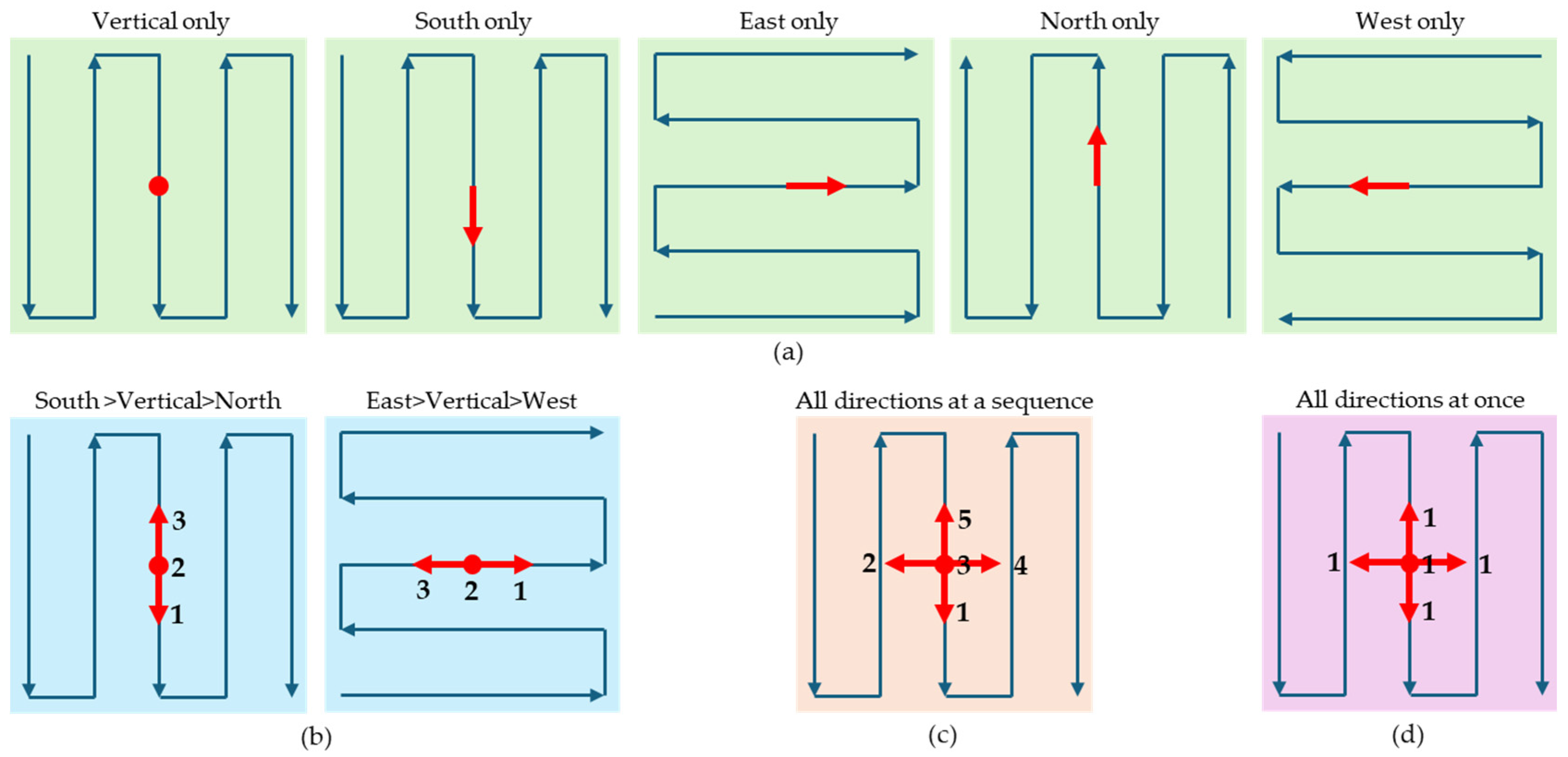
It is well known that combining oblique images with nadir-only images leads to more accurate AT. Four scenarios can be considered for nadir–oblique combined photography (Figure 1). It assumes that a single grid designates a zigzag route covering the area of interest by traversing north to south (or east to west) along with reversed directions, namely the first phase, and that a double grid includes additional routes traversing perpendicular to the first route, namely the second phase. It also assumes that oblique shots are taken in north, south, east, and west directions.

• A Single Grid for Each Direction: In this method, a maximum of five single grids can be conducted where the camera gimbal is fixed in a specific direction for each single grid. This is the least efficient method.
• Sequential Nadir/2–Oblique Shots in a Double Grid: The camera gimbal’s pitch is repeatedly adjusted to capture nadir and oblique images sequentially while flying in the first phase of a double grid. The second flight is conducted in the second phase, changing the pitch only for oblique images. This method requires a double grid flight, resulting in better efficiency and allowing for precise overlap between nadir and oblique images by targeting the same point. The DJI Mavic 3 Enterprise fits this approach.
• Sequential Nadir/4–Oblique Shots in a Single Grid: While flying in a single grid, the camera gimbal’s pitch and roll are adjusted to capture a nadir and four oblique images sequentially. This method requires only a single grid flight, making it more efficient but requiring a highly developed camera and gimbal technique. The DJI Matrice 300 fits this approach.
• Omnidirectional Shots in a Single Grid: An omnidirectional camera captures images in all directions simultaneously, enabling efficient data collection with just a single grid flight, similar to the third method. However, challenges include ensuring precise image overlap, especially if the camera lenses cannot adjust angles in real time, and accurately modeling the images when high lens distortion is present [29].

2.2. AT Based on Constraint Equation

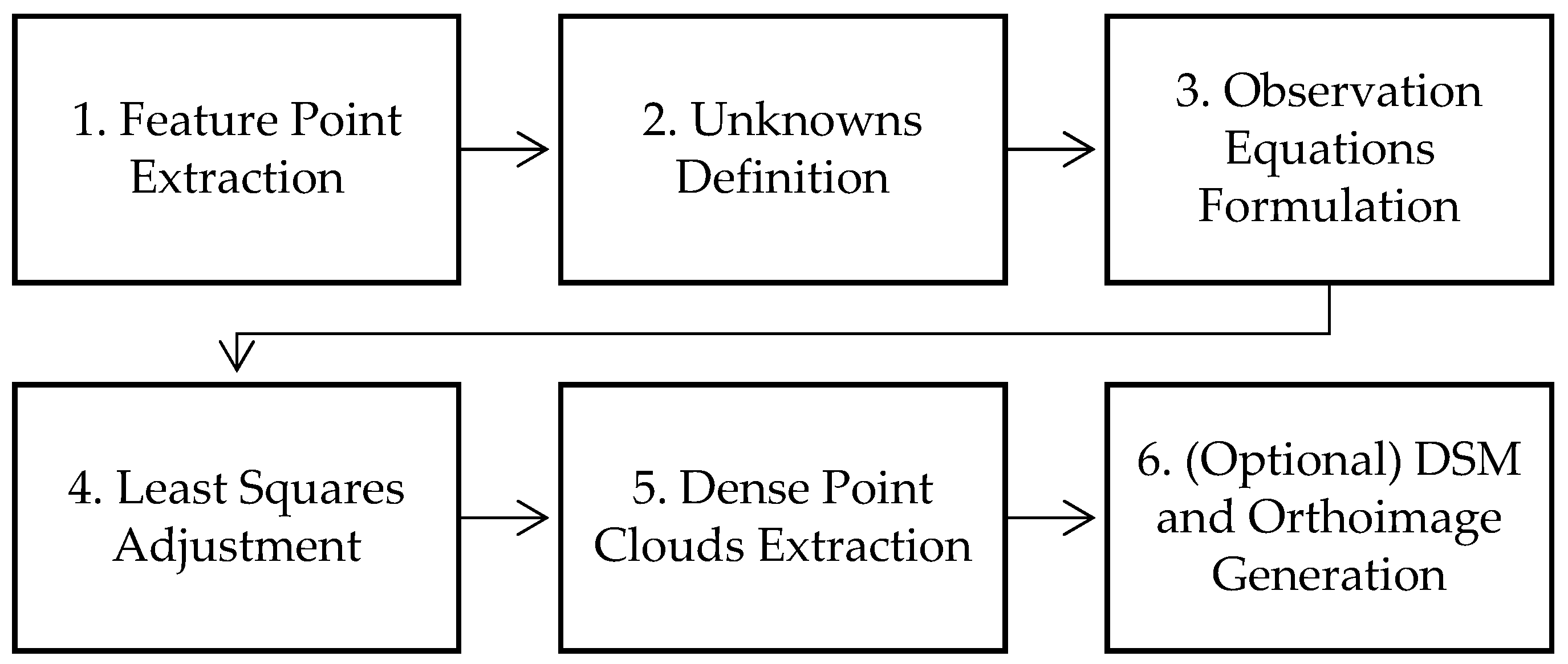
Direct georeferencing of images captured by RTK or PPK UAVs is typically conducted using SfM [30,31,32,33,34]. Although the scope and terminology for SfM can vary, several common procedures are involved (Figure 2):

• Extracting numerous feature points from each image and identifying correspondences between potential image pairs using these feature points.
• Defining unknowns, such as the 3D coordinates of conjugate points, interior orientation parameters (IOPs), EOPs, and initial values from UAV sensors.
• Formulating observation equations for each image pair based on the collinearity condition, incorporating the unknowns and initial values.
• Linearizing the equations and iteratively performing least squares adjustment to estimate the unknowns.
• Extracting dense point clouds from each registered image pair based on image matching and determining the 3D coordinates of these points.
• (Optionally) generating a digital surface model (DSM) and orthoimages or orthomosaic images.

Among the steps, weighted observations can be incorporated into the observation equations as a constraint equation in step 3. A constraint equation involves either substituting an unknown with an observed value or adding an observation equation with an assigned weight to regulate the degree of change in the unknown [35]. The former approach is used when an observation is known to be highly accurate, while the latter is applied when the observation is comparatively reliable or requires adjustment in its influence relative to others.

Using a Taylor expansion, the Jacobian matrix $J$, which is the first derivative coefficient matrix, linearizes the collinearity equation. The unknown matrix containing the EOPs for each image is represented by $X$. The constant matrix, $K$, is calculated by applying the (updated) unknown values to the observation equations, and $V$ denotes the residual matrix. The observation equation is shown in Equation (2):

$$JX=K+V$$

(2)

If the corrections $(dx, dy, dz)$ for the 3D coordinates $(x,y,z)$ in the EOPs are separated and expressed as $X_2$, Equation (2) can be reformulated with separated components, as shown in Equation (3):

$$\left[\begin{array}{cc}{J}_1& J_2\end{array}\right]\left[\begin{array}{c}{X}_1\\ X_2\end{array}\right]=\left[\begin{array}{c}{K}_1\\ K_2\end{array}\right]+\left[\begin{array}{c}{V}_1\\ V_2\end{array}\right]$$

(3)

where $X_2={\left[\begin{array}{ccc}{d}_x& d_y& d_z\end{array}\right]}^T$ and $X_1$ denotes the corrections of other unknowns.

Equation (4) provides the observation equations for applying the 3D coordinates $(x_{obs},y_{obs},z_{obs})$ measured by the RTK UAVs:

$$x=x_{obs}+v_x,y=y_{obs}+v_y,z=z_{obs}+v_z$$

(4)

Equation (5) shows the complete set of observation equations, integrating Equation (4) into Equation (3):

$$\left[\begin{array}{c}\begin{array}{cc}{J}_1& J_2\end{array}\\ \begin{array}{cc}0& I\end{array}\end{array}\right]\left[\begin{array}{c}{X}_1\\ X_2\end{array}\right]=\left[\begin{array}{c}\begin{array}{c}{K}_1\\ K_2\end{array}\\ K_3\end{array}\right]+\left[\begin{array}{c}\begin{array}{c}{V}_1\\ V_2\end{array}\\ V_3\end{array}\right]$$

(5)

where $I=\left[\begin{array}{ccc}1& 0& 0\\ 0& 1& 0\\ 0& 0& 1\end{array}\right]$, ${ K}_3={\left[\begin{array}{ccc}{x}_{obs}-x_0& y_{obs}-y_0& z_{obs}-z_0\end{array}\right]}^T$, and $V_3={\left[\begin{array}{ccc}{v}_x& v_y& v_z\end{array}\right]}^T$.

The reciprocal variance in the RTK measurements can represent the weights $W_2$ for the 3D coordinate observations. Equation (6) separates $W_2$ from the weights $W_1$ of the other unknowns:

$$W=\left[\begin{array}{c}\begin{array}{cc}{W}_1& 0\end{array}\\ \begin{array}{cc}0& W_2\end{array}\end{array}\right]$$

(6)

where $W_2=\left[\begin{array}{ccc}1/{{\sigma }_x}^2& 0& 0\\ 0& 1/{{\sigma }_y}^2& 0\\ 0& 0& {1/{\sigma }_z}^2\end{array}\right]$.

Applying Equation (6) to Equation (5) yields Equations (7) and (8).

$$W\left[\begin{array}{c}\begin{array}{cc}{J}_1& J_2\end{array}\\ \begin{array}{cc}0& I\end{array}\end{array}\right]\left[\begin{array}{c}{X}_1\\ X_2\end{array}\right]=W\left[\begin{array}{c}\begin{array}{c}{K}_1\\ K_2\end{array}\\ K_3\end{array}\right]+W\left[\begin{array}{c}\begin{array}{c}{V}_1\\ V_2\end{array}\\ V_3\end{array}\right]$$

(7)

$$\left[\begin{array}{c}\begin{array}{cc}{W}_1& 0\end{array}\\ \begin{array}{cc}0& W_2\end{array}\end{array}\right]\left[\begin{array}{c}\begin{array}{cc}{J}_1& J_2\end{array}\\ \begin{array}{cc}0& I\end{array}\end{array}\right]\left[\begin{array}{c}{X}_1\\ X_2\end{array}\right]=\left[\begin{array}{c}\begin{array}{cc}{W}_1& 0\end{array}\\ \begin{array}{cc}0& W_2\end{array}\end{array}\right]\left[\begin{array}{c}\begin{array}{c}{K}_1\\ K_2\end{array}\\ K_3\end{array}\right]+\left[\begin{array}{c}\begin{array}{cc}{W}_1& 0\end{array}\\ \begin{array}{cc}0& W_2\end{array}\end{array}\right]\left[\begin{array}{c}\begin{array}{c}{V}_1\\ V_2\end{array}\\ V_3\end{array}\right]$$

(8)

The least squares adjustment is iterated on Equation (7) until the corrections converge within specified thresholds. Adjusting the weight $W_2$ allows control over the degree of adjustment applied to the 3D coordinates. Typically, the extensible metadata platform (XMP) of images captured by RTK UAVs includes the 3D coordinates and their variances measured via RTK, along with three-axis attitude information from the camera gimbal. The accuracy of 3D coordinate measurements from RTK UAVs has reached a reliably high level, allowing these variances to be applied as weights in $W_2$ in Equations (6) and (8).

2.3. Point Cloud Filtering Based on Each Point’s Confidence

SfM, which extracts feature points from images and performs point matching using descriptors, can reduce the generation of noise points through rigorous filtering. However, challenges arise when the target surface is homogeneous with limited distinctive features, when there is movement or vibration in the target, or when the texture is overly fine and complex, which can increase noise points. Therefore, point clouds generated with SfM often require additional filtering. Common filtering methods rely on the topology among neighboring points or the local surface geometry. Additionally, each point’s confidence level can be assessed during feature extraction, point matching, and 3D position estimation, allowing filtering based on this confidence. Methods for evaluating point confidence during the production stages include the following:

• Redundancy of Stereo Pairs: While the 3D coordinates of a point can be calculated from a single image pair following AT, merging redundant disparity estimations from multiple stereo models can enhance the precision and robustness of the point clouds [36]. Thus, the extent to which 3D coordinates are calculated from multiple image pairs serves as a reliability measure.
• Geometric Distance: The reliability of point clouds can be evaluated by calculating the distance between points in the cloud and a reference plane [37,38]. This method is highly accurate but applies only under the assumption that a reference plane exists.
• Triangulation Error: The 3D coordinates of a point are calculated using collinearity conditions from a single image pair. With three unknowns in the 3D coordinates and four collinearity equations, the least squares adjustment can estimate unknown values. The residual magnitude in this process can indicate reliability. However, if image pairs are insufficient, residuals may be over- or under-estimated regardless of actual positional accuracy.
• Reprojection Error: The 3D coordinates calculated from multiple image pairs can be reprojected onto the original images by substituting them into the collinearity equations. The reliability of a point is evaluated by comparing initial image coordinates with reprojected coordinates [39]. Similar to triangulation error, this method may also lead to over- or under-estimation if there are too few image pairs.
• Texture Quality: In SfM, the scale-invariant feature transform (SIFT) extracts feature points and calculates descriptors based on the texture around each point, then matches points with similar descriptors to compute 3D coordinates [40]. When the texture has distinct and unique patterns, the matching success rate improves, making texture quality a potential reliability measure.

Methods 3–5 are inherently applied in some form during the SfM process. This study, however, focuses on filtering the point cloud by applying the first method: redundancy of stereo pairs. This method, implemented in SfM software such as Agisoft Metashape, counts the number of image pairs used to calculate the 3D coordinates of a given point. The number of image pairs can range from a minimum of two to dozens, depending on the level of image overlap. The confidence value is then normalized to a range of 0–1 or 0–255 based on the maximum and minimum overlap counts.

3. Data Acquisition and Processing

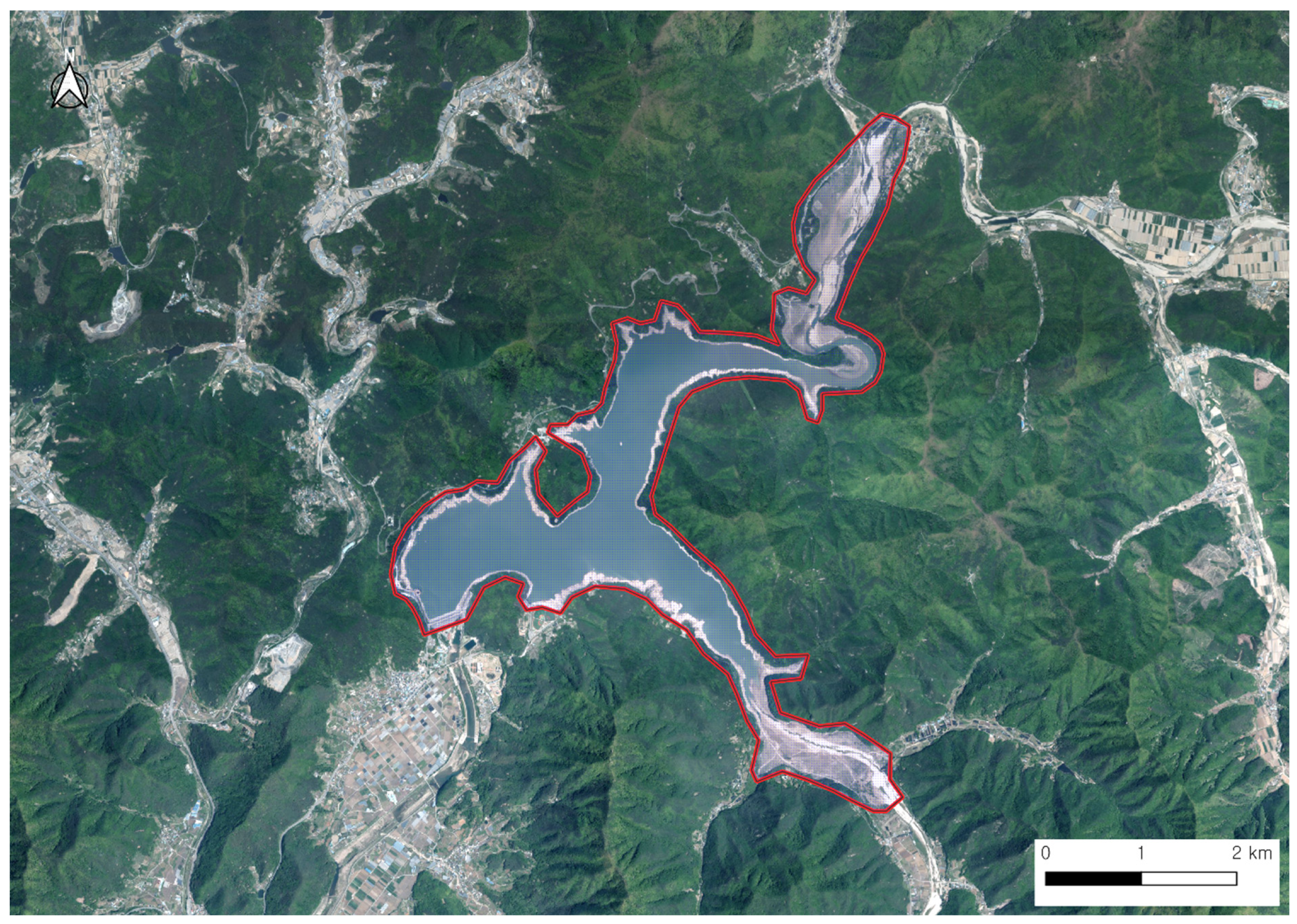
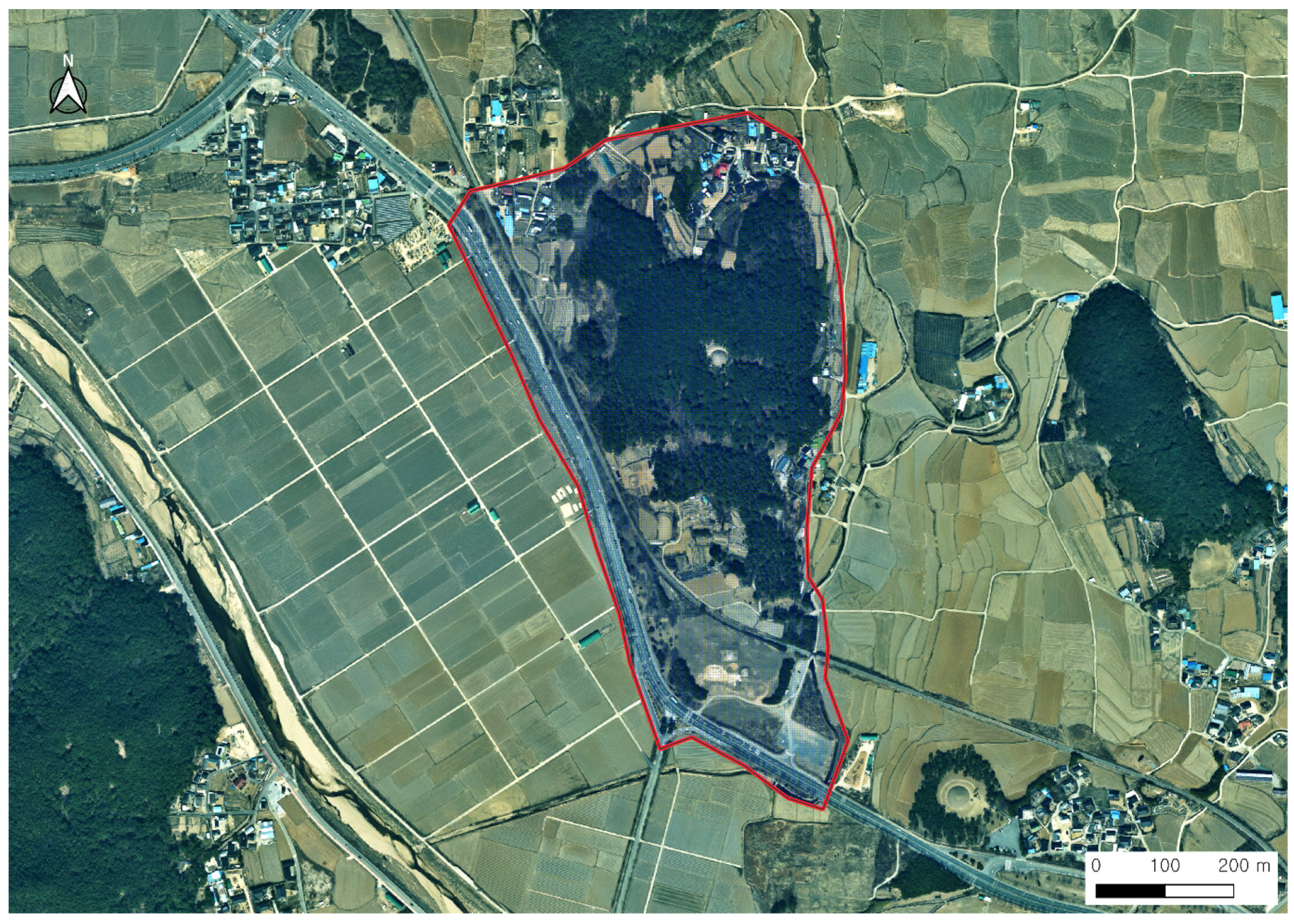
In the study area, aerial images were taken at two sites using an RTK UAV. Site 1 encompasses a dam and its basin, covering approximately 9.8 km², while Site 2 is a densely forested hill area with an area of approximately 0.3 km². The layouts of the two sites are shown in Figure 3 and Figure 4, and the general properties and specifications of the images are summarized in

Table 1. Specifications of flight missions.

Item	Site 1	Site 2
Covered area	9.8 km2	0.3 km2
Object type	Dam and basin area	Hill area
Location	Cheongdogun, Gyeongbuk, South Korea	Gyeongjusi, Gyeongbuk, South Korea
Latitude, longitude	35.734724°, 128.940673°	35.8224338°, 129.2423647°
Flight altitude	145 m (constant)	65 m (adjusted for terrain)
Nadir GSD	4.5 cm/pixel	2.0 cm/pixel
Oblique angle from nadir	20~30°	45°
Overlap/sidelap (%)	80/70	90/80
Flight speed	5~15 m/s	5~15 m/s
RTK method	NTRIP provided by National Geographic Information Institute, Republic of Korea

. The specifications of the RTK UAV are provided in

Table 2. Specifications of the RTK UAV.

Item	Value
Model	DJI Mavic 3 Enterprise (3E)
GNSS signal	GPS/Galileo/BeiDou/GLONASS
RTK accuracy	1 cm + 1 ppm (horizontal), 1.5 cm + 1 ppm (vertical)
Sensor	DJI M3E, 4/3 inch CMOS, 20 mega effective pixel
Field of view	84°
Image dimension	5280 × 3956 pixels

.

The accuracy of AT was evaluated by calculating the root mean square error (RMSE) for checkpoints in the final orthomosaic image. Additionally, accuracy comparisons were performed under various conditions: excluding oblique images, omitting high weighting for 3D coordinates, and not applying point cloud filtering. Similar tests were also conducted on more moderate terrain, characterized by hills without water surfaces, in order to assess the effects of these methods in diverse environmental settings.

Due to the large area of Site 1, covering it with a multicopter UAV posed challenges. The operation took three days, using a single UAV with multiple batteries recharged sequentially after each flight. To enhance flight efficiency, the altitude was kept at approximately 145 m above the starting point, without adjustments for terrain variation. The DJI Mavic 3 Enterprise supports the “Sequential Nadir/2–Oblique Shots in a Double Grid” function described in Section 2.1.4. However, to complete the mission within the allotted time, only the first phase of the double-grid method was used. As noted in [10], increasing the oblique angle typically improves vertical accuracy, and the UAV can capture images at angles of up to 45°. However, achieving a 45° oblique angle would have required expanding the flight area. Due to the surrounding mountainous terrain reaching the flight altitude, the oblique angle was limited to 20–30° for flight safety.

For Site 2, a relatively smaller area, the altitude was adjusted in real time to consistently maintain 65 m above the immediate terrain. The “Sequential Nadir/2–Oblique Shots in a Double Grid” method was applied in both phases with a 45° oblique angle. For both sites, all settings—including flight speed, shutter speed, aperture, ISO sensitivity, and focusing—were set to automatic mode to adapt to varying light and environmental conditions over the extended mission duration. Even at maximum UAV speed, pixel smearing remained within two pixels. DJI Pilot (version 02.01.0517) software’s smart oblique function was used to ensure precise overlap between nadir and oblique images.

To assess the accuracy of AT, four methods were tested based on the application of specific weights to the 3D coordinates of the EOPs in the constraint equation and the inclusion of oblique images:

• Nadir–oblique image combination with specific weights.
• Nadir–oblique image combination with equal weights.
• Nadir images only with specific weights.
• Nadir images only with equal weights.

In methods 1 and 3, the 3D coordinates (longitude, latitude, ellipsoid height) extracted from the XMP metadata of the RTK UAV images were used as observations in the constraint equation, with variances $({{\sigma }_x}^2,{{\sigma }_y}^2,{{\sigma }_z}^2)$ from the XMP applied as weights $W_2$ in Equation (5). In methods 2 and 4, the 3D coordinates were also used as observations, but a large standard deviation ($\sigma =10$ m) was assigned to the variances, reducing the weights $W_2$ and allowing SfM greater flexibility in adjusting the 3D coordinates. Additionally, in all methods, a large standard deviation ($\sigma =10$°) was applied to the variances for the three-axis attitudes (roll, pitch, yaw) to permit broader adjustments. The specific factors and number of images used in each method are summarized in

Table 3. Detailed factors and number of images applied to each method for Site 1.

	Method 1	Method 2	Method 3	Method 4
${\sigma }_x\left(\mathrm{m}\right)$	0.0074~0.0174	10	0.0075~0.0174	10
${\sigma }_y\left(\mathrm{m}\right)$	0.0084~0.0229	10	0.0084~0.0229	10
${\sigma }_z\left(\mathrm{m}\right)$	0.0181~0.0370	10	0.0182~0.0370	10
${\sigma }_{attitude}(°)$	10	10	10	10
Nadir images	6284	6284	6284	6284
Oblique images	11,658	11,658	N/A	N/A

and

Table 4. Detailed factors and number of images applied to each method for Site 2.

	Method 1	Method 2	Method 3	Method 4
${\sigma }_x\left(\mathrm{m}\right)$	0.0080~0.0264	10	0.0081~0.0160	10
${\sigma }_y\left(\mathrm{m}\right)$	0.0076~0.0268	10	0.0080~0.0268	10
${\sigma }_z\left(\mathrm{m}\right)$	0.0201~0.0729	10	0.0206~0.0519	10
${\sigma }_{attitude}(°)$	10	10	10	10
Nadir images	1302	1302	1302	1302
Oblique images	5823	5823	N/A	N/A

.

After completing AT, point clouds and a digital surface model (DSM) were generated. An orthomosaic image was then created, and accuracy was assessed using checkpoints. Additionally, confidence values for each point in the point cloud were extracted, with points below a certain threshold identified as noise and removed. The DSM and orthomosaic image were recreated to re-evaluate accuracy with the checkpoints. All processes were conducted using Agisoft Metashape. The specifications of the processing system and overall processing time for Method 1 are provided in

Table 5. Specifications of the processing system and overall processing time.

	Site 1	Site 2
CPU	AMD Ryzen 9 7950X 16-Core Processor 4.50 GHz
GPUs	NVIDIA RTX 4070 Ti 2 ea	NVIDIA RTX 4080 2 ea
Operating system	Windows 11
SfM software	Agisoft Metashape 2.1.2
Processing time	13 h 10 min	9 h 16 min

.

4. Results

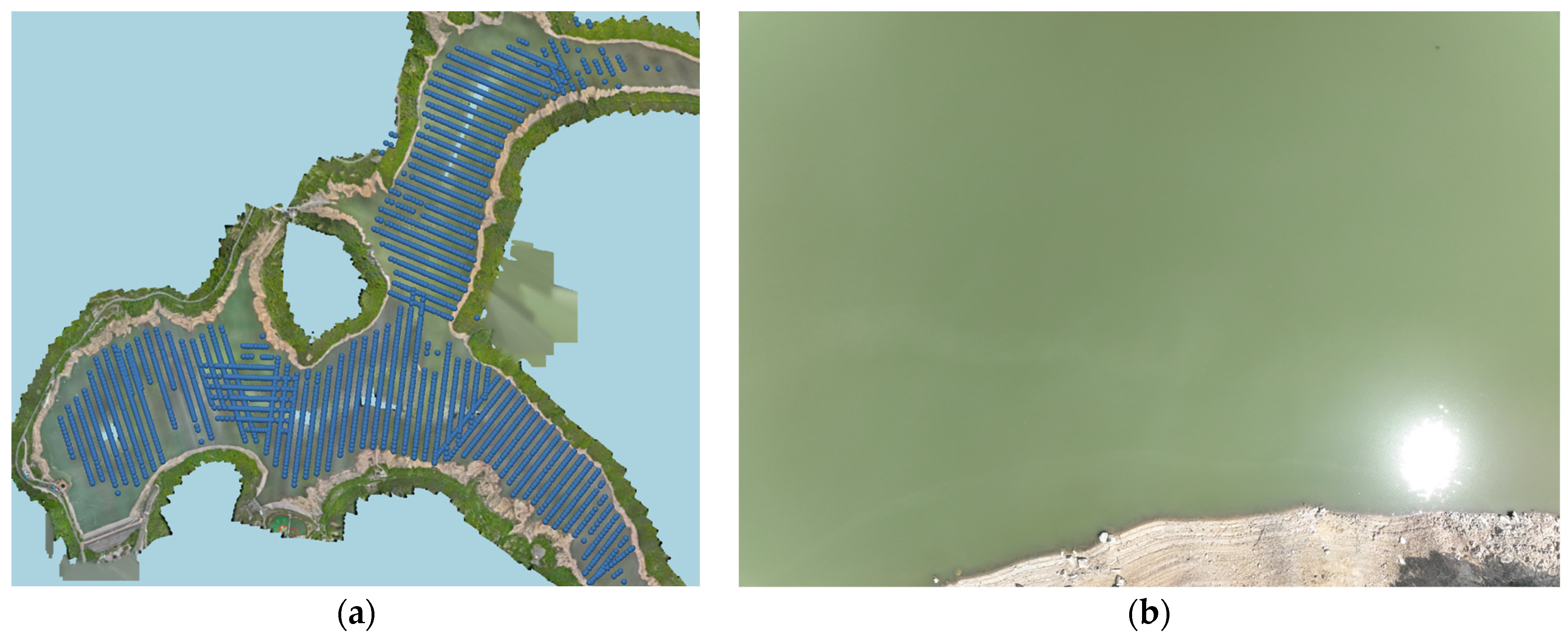
At Site 1, feature point extraction and image matching over the water surface posed significant challenges, resulting in numerous images failing during AT and subsequent processing. These failed images accounted for 4110 out of a total of 17,942, representing 23% of the images (Figure 5). In contrast, Site 2 had relatively favorable conditions, allowing for successful processing of all images.

Table 6. Average absolute adjustment values for 3D coordinates in EOPs at Site 1.

	Method 1	Method 2	Method 3	Method 4
$dx\left(\mathrm{m}\right)$	0.0011	0.1080	0.0005	0.1719
$dy\left(\mathrm{m}\right)$	0.0012	0.1938	0.0006	0.2258
$dz\left(\mathrm{m}\right)$	0.0103	0.4661	0.0091	0.5127

and

Table 7. Average absolute adjustment values for 3D coordinates in EOPs at Site 2.

	Method 1	Method 2	Method 3	Method 4
$dx\left(\mathrm{m}\right)$	0.0068	0.0313	0.0015	0.1116
$dy\left(\mathrm{m}\right)$	0.0053	0.0262	0.0017	0.0788
$dz\left(\mathrm{m}\right)$	0.0190	0.0295	0.0213	0.4225

present the average absolute adjustment values for the 3D coordinates in the EOPs across Methods 1–4. As expected, the adjustments were relatively small in Methods 1 and 3, while they were significantly larger in Methods 2 and 4.

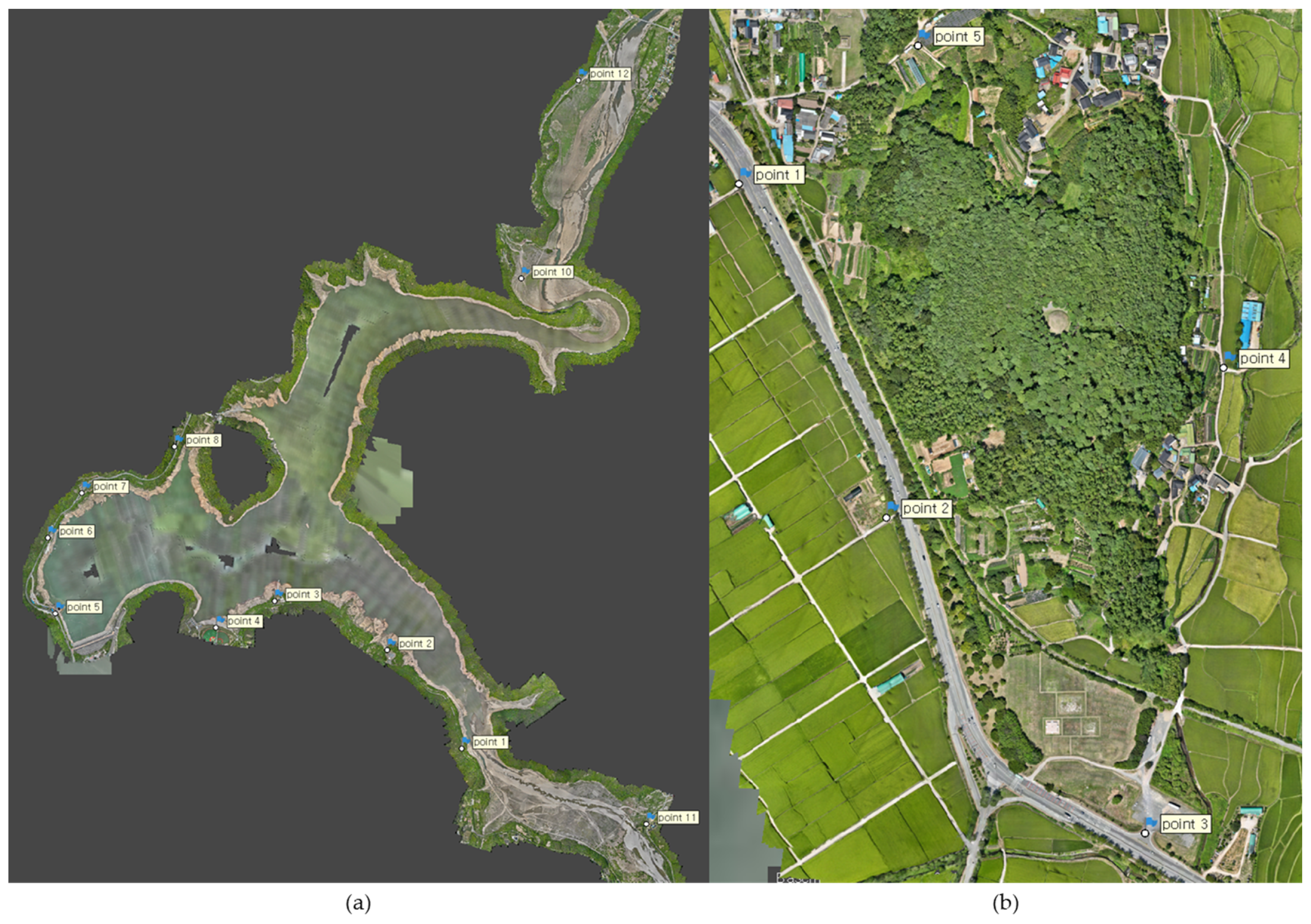
In total, 12 checkpoints were collected at Site 1 and 5 at Site 2 (Figure 6). The RMSEs estimated for the checkpoints are summarized in

Table 8. RMSEs for checkpoints at Site 1.

	Method 1	Method 2	Method 3	Method 4
$x\left(\mathrm{m}\right)$	0.0155	0.7543	0.0219	0.2745
$y\left(\mathrm{m}\right)$	0.0219	0.7801	0.0259	0.2275
$z\left(\mathrm{m}\right)$	0.1419	0.9361	0.3670	0.5623
$3\mathrm{D}\left(\mathrm{m}\right)$	0.1444	1.4331	0.3686	0.6658

and

Table 9. RMSEs for checkpoints at Site 2.

	Method 1	Method 2	Method 3	Method 4
$x\left(\mathrm{m}\right)$	0.0165	0.0347	0.0172	0.1688
$y\left(\mathrm{m}\right)$	0.0206	0.0308	0.0229	0.3229
$z\left(\mathrm{m}\right)$	0.0345	0.0424	0.0551	0.7042
$3\mathrm{D}\left(\mathrm{m}\right)$	0.0434	0.0629	0.0621	0.7929

. At Site 1, Method 1 achieved the highest accuracy, with Method 3 also showing reasonable horizontal accuracy. In contrast, Methods 2 and 4 exhibited significant deviations from the typical accuracy expected in RTK positioning. Similarly, at Site 2, Method 1 achieved the highest accuracy, while Method 3 demonstrated satisfactory accuracy. Unlike Site 1, Method 2 at Site 2 showed accuracy levels comparable to Method 3.

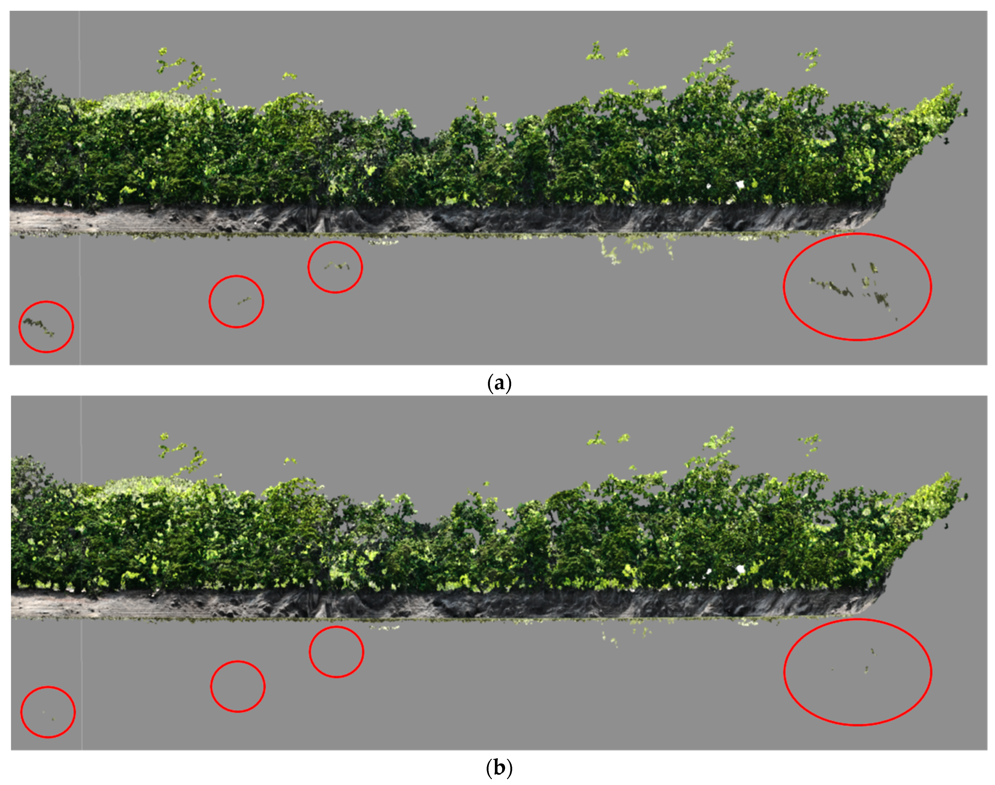
Next, accuracy was evaluated by filtering the point cloud based on confidence values. At Site 1, the extensive water bodies in the images posed challenges for feature point extraction, and sunlight-induced speckling frequently led to matching errors. Additionally, surrounding trees and windy conditions during the flight increased the likelihood of these errors. Figure 7 and Figure 8 show the point clouds before and after confidence-based filtering at Site 1, demonstrating that error points from matching issues can be identified and removed relatively easily. Confidence values were calculated in Metashape, using the redundancy of stereo pairs as described in the previous section. The filtering criteria for this study were heuristically set based on empirical observations.

Point cloud filtering and accuracy assessments were applied only to Method 1, and the RMSEs for the checkpoints are summarized in

Table 10. RMSEs for checkpoints before and after filtering.

	Site 1		Site 2
	Before Filtering	After Filtering	Before Filtering	After Filtering
$x\left(\mathrm{m}\right)$	0.0155	0.0155	0.0165	0.0187
$y\left(\mathrm{m}\right)$	0.0219	0.0213	0.0206	0.0195
$z\left(\mathrm{m}\right)$	0.1419	0.1419	0.0345	0.0345
$3\mathrm{D}\left(\mathrm{m}\right)$	0.1444	0.1443	0.0434	0.0438

. Filtering had minimal impact on accuracy at both Site 1 and Site 2, likely because error points were located far from the checkpoints. Although filtering did not improve accuracy, it is noteworthy that accuracy was not reduced by the removal of potentially valid points.

5. Discussion

As previously indicated, the extensive area of Site 1 necessitated limiting flights to a single phase, with images captured at moderate resolution, with overlap, and at oblique angles to enhance flight efficiency. Furthermore, the site was predominantly covered with water, which impeded SfM from extracting a sufficient number of feature points and generating accurate correspondences. As mentioned in the Introduction, incorporating oblique images in general environments typically enhances accuracy. However, in this specific situation, oblique images amplified the effects of sunlight-induced speckling and perspective distortion, which ultimately reduced accuracy [12]. As a result, Method 2, which utilized oblique images, performed worse than Method 4, which relied solely on vertical images. Consequently, SfM alone was unable to achieve acceptable accuracy without applying adjusted weights to the 3D coordinates in the EOPs within the constraint equation. Nevertheless, with the application of adjusted weights, satisfactory results were obtained, emphasizing the critical role of applying specific weights to constraint equations in complex environments such as Site 1.

In contrast, the generally higher accuracy at Site 2 can be attributed to several favorable factors, such as land cover and an enhanced ground sampling distance, which supported successful feature point extraction and image matching. Additionally, a two-phase double-grid flight, higher overlap, and a larger oblique angle contributed positively to the results. These conditions support SfM, suggesting that reasonable accuracy can be obtained even without applying specific weights to constraint equations.

A visual inspection of the point cloud at Site 1 reveals the presence of erroneous points resulting from image matching, highlighting the necessity for filtering. Point cloud filtering is a well-researched area, with numerous established methods available. Unless the site is sufficiently small for erroneous points to impact AT, or such error points are widespread across the area, the accuracy of AT is unlikely to be significantly affected by the application of filtering, as evidenced by the results from Sites 1 and 2. Consequently, filtering constitutes an essential step in SfM to ensure a high-quality point cloud.

The following insights can be drawn from the discussion:

• SfM emphasizes the relative orientation between overlapping images, often resulting in excellent stereo model alignment. However, this approach does not always ensure absolute positioning accuracy due to error propagation.
• For high-accuracy AT using RTK UAVs, adjusting the weights of RTK-observed 3D coordinates in the constraint equations is essential.
• Including oblique images can positively impact absolute positioning accuracy. However, under conditions unfavorable for SfM, it may exacerbate error propagation and reduce accuracy if the weight-adjustment approach is not applied.
• Confidence-based point cloud filtering effectively identifies and removes error points in areas with challenging image matching, with no clear positive or negative impact on geometric accuracy based on the current experimental results.

6. Conclusions

With advancements in UAV dynamics, positioning accuracy, and imaging performance, the scope of UAV-based mapping and 3D modeling continues to expand. SfM, a computer vision-based approach, is increasingly replacing traditional photogrammetry as it allows for automated AT, terrain modeling, and orthomosaic generation from large volumes of aerial imagery. This study analyzed and applied methodologies to improve the accuracy of SfM-based AT using RTK UAV imagery for large-scale infrastructure projects, yielding significant insights:

• In SfM-based AT, a constraint equation was applied by adjusting weights according to the observed variances in 3D coordinates from RTK UAVs. This method effectively reduced error propagation within SfM, achieving high AT accuracy. However, as no software currently offers explicit guidelines for integrating RTK UAV observations into AT, it is essential to verify that each software package accurately implements this method to achieve relevant AT accuracy.
• The inclusion of oblique images, combined with the weight-adjustment approach, significantly improved AT accuracy. Actively using UAVs that can capture both nadir and oblique images simultaneously, without compromising mission efficiency, is highly recommended.
• Due to the nature of SfM, errors may arise in environments where image matching is challenging, resulting in numerous error points. Filtering point clouds based on confidence values can enhance their geometric quality. Therefore, it is recommended that point clouds generated through SfM undergo reliability assessment and filtering.

Future work will focus on creating a more objective process for filtering point clouds based on confidence values. Additionally, following recommendations from the relevant literature [41], it will be important to assess AT accuracy under varying RTK positioning reliability conditions. Efforts will also be directed toward developing or adopting UAVs optimized for more efficient oblique photography.

References

- Ahmed, R.; Mahmud, K.H. Potentiality of High-Resolution Topographic Survey Using Unmanned Aerial Vehicle in Bangladesh. Remote Sens. Appl. Soc. Environ. 2022, 26, 100729. [Google Scholar] [CrossRef]
- Cirillo, D.; Zappa, M.; Tangari, A.C.; Brozzetti, F.; Ietto, F. Rockfall Analysis from UAV-Based Photogrammetry and 3D Models of a Cliff Area. Drones 2024, 8, 31. [Google Scholar] [CrossRef]
- Molina, A.A.; Huang, Y.; Jiang, Y. A Review of Unmanned Aerial Vehicle Applications in Construction Management: 2016–2021. Standards 2023, 3, 95–109. [Google Scholar] [CrossRef]
- Halik, Ł.; Smaczyński, M. Geovisualisation of Relief in a Virtual Reality System on the Basis of Low-Level Aerial Imagery. Pure Appl. Geophys. 2018, 175, 3209–3221. [Google Scholar] [CrossRef]
- Salem, T.; Dragomir, M.; Chatelet, E. Strategic Integration of Drone Technology and Digital Twins for Optimal Construction Project Management. Appl. Sci. 2024, 14, 4787. [Google Scholar] [CrossRef]
- Villanueva, J.K.S.; Blanco, A.C. Optimization of Ground Control Point (GCP) Configuration for Unmanned Aerial Vehicle (UAV) Survey Using Structure from Motion (SFM). Int. Arch. Photogramm. Remote Sens. Spat. Inf. Sci. 2019, 42, 167–174. [Google Scholar] [CrossRef]
- Cramer, M.; Stallmann, D.; Haala, N. Direct Georeferencing Using GPS/Inertial Exterior Orientations for Photogrammetric Applications. Int. Arch. Photogramm. Remote Sens. 2000, 33, 198–205. [Google Scholar]
- Štroner, M.; Urban, R.; Seidl, J.; Reindl, T.; Brouček, J. Photogrammetry Using UAV-Mounted GNSS RTK: Georeferencing Strategies without GCPs. Remote Sens. 2021, 13, 1336. [Google Scholar] [CrossRef]
- Fazeli, H.; Samadzadegan, F.; Dadrasjavan, F. Evaluating the Potential of RTK-UAV for Automatic Point Cloud Generation in 3D Rapid Mapping. Int. Arch. Photogramm. Remote Sens. Spatial Inf. Sci. 2016, 41, 221–226. [Google Scholar] [CrossRef]
- Tomaštík, J.; Mokroš, M.; Surový, P.; Grznárová, A.; Merganič, J. UAV RTK/PPK Method—An Optimal Solution for Mapping Inaccessible Forested Areas? Remote Sens. 2019, 11, 721. [Google Scholar] [CrossRef]
- Jaud, M.; Bertin, S.; Beauverger, M.; Augereau, E.; Delacourt, C. RTK GNSS-Assisted Terrestrial SfM Photogrammetry without GCP: Application to Coastal Morphodynamics Monitoring. Remote Sens. 2020, 12, 1889. [Google Scholar] [CrossRef]
- Chen, C.; Tian, B.; Wu, W.; Duan, Y.; Zhou, Y.; Zhang, C. UAV Photogrammetry in Intertidal Mudflats: Accuracy, Efficiency, and Potential for Integration with Satellite Imagery. Remote Sens. 2023, 15, 1814. [Google Scholar] [CrossRef]
- Zhang, H.; Aldana-Jague, E.; Clapuyt, F.; Wilken, F.; Vanacker, V.; Van Oost, K. Evaluating the Potential of Post-Processing Kinematic (PPK) Georeferencing for UAV-Based Structure-from-Motion (SfM) Photogrammetry and Surface Change Detection. Earth Surf. Dynam. 2019, 7, 807–827. [Google Scholar] [CrossRef]
- Štroner, M.; Urban, R.; Reindl, T.; Seidl, J.; Brouček, J. Evaluation of the Georeferencing Accuracy of a Photogrammetric Model Using a Quadrocopter with Onboard GNSS RTK. Sensors 2020, 20, 2318. [Google Scholar] [CrossRef]
- Liu, X.; Lian, X.; Yang, W.; Wang, F.; Han, Y.; Zhang, Y. Accuracy Assessment of a UAV Direct Georeferencing Method and Impact of the Configuration of Ground Control Points. Drones 2022, 6, 30. [Google Scholar] [CrossRef]
- Nota, E.W.; Nijland, W.; de Haas, T. Improving UAV-SfM Time-Series Accuracy by Co-Alignment and Contributions of Ground Control or RTK Positioning. Int. J. Appl. Earth Obs. Geoinf. 2022, 109, 102772. [Google Scholar] [CrossRef]
- Han, S.; Hong, C.-K. Accuracy Assessment of Aerial Triangulation of Network RTK UAV. J. Korean Soc. Surv. Geod. Photogramm. Cartogr. 2020, 38, 663–670. [Google Scholar] [CrossRef]
- Cho, J.; Lee, J.; Lee, B. A Study on the Accuracy Evaluation of UAV Photogrammetry using Oblique and Vertical Images. J. Korean Soc. Surv. Geod. Photogramm. Cartogr. 2021, 39, 41–46. [Google Scholar] [CrossRef]
- Rehak, M.; Mabillard, R.; Skaloud, J. A Micro-Uav with the Capability Ff Direct Georeferencing. Int. Arch. Photogramm. Remote Sens. Spat. Inf. Sci. 2013, 40, 317–323. [Google Scholar] [CrossRef]
- Turner, D.; Lucieer, A.; Wallace, L. Direct Georeferencing of Ultrahigh-Resolution UAV Imagery. IEEE Trans. Geosci. Remote Sens. 2014, 52, 2738–2745. [Google Scholar] [CrossRef]
- Gabrlik, P. The Use of Direct Georeferencing in Aerial Photogrammetry with Micro UAV. IFAC-PapersOnLine 2015, 48, 380–385. [Google Scholar] [CrossRef]
- Masiero, A.; Fissore, F.; Vettore, A. A Low Cost UWB Based Solution for Direct Georeferencing UAV Photogrammetry. Remote Sens. 2017, 9, 414. [Google Scholar] [CrossRef]
- Ekaso, D.; Nex, F.; Kerle, N. Accuracy Assessment of Real-Time Kinematics (RTK) Measurements on Unmanned Aerial Vehicles (UAV) for Direct Geo-Referencing. Geo-Spat. Inf. Sci. 2020, 23, 165–181. [Google Scholar] [CrossRef]
- Toscano, F.; Fiorentino, C.; Capece, N.; Erra, U.; Travascia, D.; Scopa, A.; Drosos, M.P.; Drosos, M.P. D’Antonio Unmanned Aerial Vehicle for Precision Agriculture: A Review. IEEE Access 2024, 12, 69188–69205. [Google Scholar] [CrossRef]
- Czyża, S.; Szuniewicz, K.; Kowalczyk, K.; Dumalski, A.; Ogrodniczak, M.; Zieleniewicz, Ł. Assessment of Accuracy in Unmanned Aerial Vehicle (UAV) Pose Estimation with the REAL-Time Kinematic (RTK) Method on the Example of DJI Matrice 300 RTK. Sensors 2023, 23, 2092. [Google Scholar] [CrossRef]
- Greenwood, W.W.; Lynch, J.P.; Zekkos, D. Applications of UAVs in Civil Infrastructure. J. Infrastruct. Syst. 2019, 25, 04019002. [Google Scholar] [CrossRef]
- Han, S.; Hong, C.-K. Acquisition of Subcentimeter GSD Images Using UAV and Analysis of Visual Resolution. J. Korean Soc. Surv. Geod. Photogramm. Cartogr. 2017, 35, 563–572. [Google Scholar] [CrossRef]
- Han, S. Improvement of an LCD-Based Calibration Site for Reliable Focus-Dependent Camera Calibration. KSCE J. Civ. Eng. 2022, 26, 1365–1375. [Google Scholar] [CrossRef]
- Scaramuzza, D. Omnidirectional Camera. In Computer Vision: A Reference Guide; Ikeuchi, K., Ed.; Springer International Publishing: Cham, Switzerland, 2021; pp. 900–909. ISBN 978-3-030-63416-2. [Google Scholar]
- Carbonneau, P.E.; Dietrich, J.T. Cost-Effective Non-Metric Photogrammetry from Consumer-Grade sUAS: Implications for Direct Georeferencing of Structure from Motion Photogrammetry. Earth Surf. Process. Landf. 2017, 42, 473–486. [Google Scholar] [CrossRef]
- Rabah, M.; Basiouny, M.; Ghanem, E.; Elhadary, A. Using RTK and VRS in Direct Geo-Referencing of the UAV Imagery. NRIAG J. Astron. Geophys. 2018, 7, 220–226. [Google Scholar] [CrossRef]
- Woo, H.; Baek, S.; Hong, W.; Chung, M.; Kim, H.; Hwang, J. Evaluating Ortho-Photo Production Potentials Based on UAV Real-Time Geo-Referencing Points. Spat. Inf. Res. 2018, 26, 639–646. [Google Scholar] [CrossRef]
- Kim, H.; Hyun, C.-U.; Park, H.-D.; Cha, J. Image Mapping Accuracy Evaluation Using UAV with Standalone, Differential (RTK), and PPP GNSS Positioning Techniques in an Abandoned Mine Site. Sensors 2023, 23, 5858. [Google Scholar] [CrossRef] [PubMed]
- Erol, B.; Turan, E.; Erol, S.; Alper Kuçak, R. Comparative Performance Analysis of Precise Point Positioning Technique in the UAV—Based Mapping. Measurement 2024, 233, 114768. [Google Scholar] [CrossRef]
- Ghilani, C.D.; Wolf, P.R. Constraint Equations. In Adjustment Computations; Ghilani, C.D., Wolf, P.R., Eds.; Wiley Online Library: Hoboken, NJ, USA, 2006; pp. 388–408. ISBN 978-0-470-12149-8. [Google Scholar]
- Rothermel, M.; Wenzel, K.; Fritsch, D.; Haala, N. SURE: Photogrammetric Surface Reconstruction from Imagery. In Proceedings of the LC3D Workshop, Berlin, Germany, 4–5 December 2012; pp. 1–9. [Google Scholar]
- Seitz, S.M.; Curless, B.; Diebel, J.; Scharstein, D.; Szeliski, R. A Comparison and Evaluation of Multi-View Stereo Reconstruction Algorithms. In Proceedings of the 2006 IEEE Computer Society Conference on Computer Vision and Pattern Recognition (CVPR’06), New York, NY, USA, 17–22 June 2006; Volume 1, pp. 519–528. [Google Scholar]
- Furukawa, Y.; Ponce, J. Accurate, Dense, and Robust Multiview Stereopsis. IEEE Trans. Pattern Anal. Mach. Intell. 2010, 32, 1362–1376. [Google Scholar] [CrossRef] [PubMed]
- Hartley, R.; Zisserman, A. Multiple View Geometry in Computer Vision, 2nd ed.; Cambridge University Press: Cambridge, UK, 2004; ISBN 978-0-521-54051-3. [Google Scholar]
- Lowe, D.G. Distinctive Image Features from Scale-Invariant Keypoints. Int. J. Comput. Vis. 2004, 60, 91–110. [Google Scholar] [CrossRef]
- Cho, J.M.; Lee, B.K. GCP and PPK Utilization Plan to Deal with RTK Signal Interruption in RTK-UAV Photogrammetry. Drones 2023, 7, 265. [Google Scholar] [CrossRef]
Figure 1.
Four scenarios for nadir–oblique combined photography: (a) a single grid for each direction, (b) sequential nadir/2–oblique shots in a double grid, (c) sequential nadir/4–oblique shots in a single grid, and (d) omnidirectional shots in a single grid.
Figure 2.
Common procedures of SfM.
Figure 3.
Overview of Site 1 (basemap generated using the V-World API).
Figure 4.
Overview of Site 2 (basemap generated using the V-World API).
Figure 5.
Failed images at Site 1: (a) image locations; (b) a sample image.
Figure 6.
Locations of checkpoints: (a) Site 1; (b) Site 2.
Figure 7.
Point clouds with error points from a horizontal view at Site 1: (a) before filtering; (b) after filtering.
Figure 8.
Point clouds with error points from a perspective view at Site 1: (a) before filtering; (b) after filtering.