Abstract
Unmanned Aerial Vehicles (UAVs), also known as drones, have advanced greatly in recent years. There are many ways in which drones can be used, including transportation, photography, climate monitoring, and disaster relief. The reason for this is their high level of efficiency and safety in all operations. While the design of drones strives for perfection, it is not yet flawless. When it comes to detecting and preventing collisions, drones still face many challenges. In this context, this paper describes a methodology for developing a drone system that operates autonomously without the need for human intervention. This study applies reinforcement learning algorithms to train a drone to avoid obstacles autonomously in discrete and continuous action spaces based solely on image data. The novelty of this study lies in its comprehensive assessment of the advantages, limitations, and future research directions of obstacle detection and avoidance for drones, using different reinforcement learning techniques. This study compares three different reinforcement learning strategies—namely, Deep Q-Networks (DQN), Proximal Policy Optimization (PPO), and Soft Actor-Critic (SAC)—that can assist in avoiding obstacles, both stationary and moving; however, these strategies have been more successful in drones. The experiment has been carried out in a virtual environment made available by AirSim. Using Unreal Engine 4, the various training and testing scenarios were created for understanding and analyzing the behavior of RL algorithms for drones. According to the training results, SAC outperformed the other two algorithms. PPO was the least successful among the algorithms, indicating that on-policy algorithms are ineffective in extensive 3D environments with dynamic actors. DQN and SAC, two off-policy algorithms, produced encouraging outcomes. However, due to its constrained discrete action space, DQN may not be as advantageous as SAC in narrow pathways and twists. Concerning further findings, when it comes to autonomous drones, off-policy algorithms, such as DQN and SAC, perform more effectively than on-policy algorithms, such as PPO. The findings could have practical implications for the development of safer and more efficient drones in the future.
1. Introduction
UAVs are reshaping the aviation industry and have emerged as the potential successors of conventional aircraft. Without the assistance of a pilot, they are proving to be extremely convenient when it comes to reaching the most remote regions. Due to their great abilities, such as flexibility, lightweight, high mobility, and effective concealment, drones were initially most often associated with the military [1]. In spite of this, technological advancements in the past decade have led to an exponential increase in drone use, and drones are no longer used only for military purposes. Data collection, delivery, and sharing can be achieved efficiently and relatively inexpensively with UAVs, which can be customized with cutting-edge detection and surveying systems [2]. Today, drones are available in a variety of shapes, sizes, ranges, specifications, and equipment. They serve a variety of purposes, such as transporting commodities, taking photos and videos, monitoring climate change, and conducting search operations after natural disasters [3]. The development of UAVs has a significant impact on the market and economy and a variety of industries.
Despite drones being available for a long time, research on their abilities for autonomous obstacle avoidance has only recently gained attention from the scientific community. As the name implies, autonomous systems are those that can perform specific tasks without the direct intervention of a human being. The use of autonomous systems is on the rise to reduce human error and improve the efficiency of operations [4]. Humans are heavily involved in most drone practices. Drones with autonomous capabilities, however, can be extremely useful in emergency situations since they provide immediate situational awareness and direct response efforts without the need to have a pilot on-site. Security and inspection issues can also be addressed using autonomous drone systems. With predefined GPS coordinates for the departure and destination, researchers initially focused on self-navigation drones that could determine the optimal route and arrive at a predetermined location without human assistance [5]. Despite the GPS navigation claim of collision avoidance, it is still possible for a drone to collide with a tree, a building, or another drone during its flight.
Different approaches have been taken by researchers for collision avoidance. Visual stereo or monocular camera is used in obtaining depth measurements for obstacle avoidance and mapping tasks [6]. Instead of solely relying only on the visual device, researchers have also employed other types of sensors. For instance, laser range finders could give range measurements for obstacle identification and mapping of 3D environments, or ultrasonic sensors could be directly incorporated into obstacle detection operations [6]. However, the transmitting device needed for such sensors makes them too heavy for small or medium-sized UAVs. Visual sensors are not constrained by geographic conditions or locations, consequently making them less susceptible to radiation or signal interference [7]. In addition to being compact, lightweight, and energy-efficient, the cameras also offer rich information about the environment [8]. Therefore, employing only visual sensors for obstacle detection is the best option for small or medium-sized UAVs. Different strategies have been implemented in vision-based navigation systems to tackle the problem of obstacle detection and avoidance. The most popular ones, among others, are based on geometric relations, fuzzy logic, potential fields, and neural networks [9].
In recent years, the field of deep reinforcement learning (DRL) has experienced exponential growth in both its research and applications. Reinforcement learning (RL) can address a variety of complicated decision-making tasks that were previously beyond the capacity of a machine to function like a human and solve problems in the real world. The ability of autonomous drones to detect and avoid obstacles with a high degree of accuracy is considered a challenging task. Applying reinforcement learning in averting collisions can provide a model which can dynamically adapt to the environment. In RL-based techniques, the agent attempts to learn in a virtual world that is analogous to a real-world setting, and then the trained model is applied to a real drone for testing [10]. When training RL models for effective collision avoidance, it is imperative to minimize the gap between the real world and the training environment. There should be a close correlation between the training environment and the real world. Different obstacle avoidance scenarios should be taken into account during training. Choosing the best reinforcement learning model is essential to obtaining the best result.
The purpose of this study is to explore the use of reinforcement learning models to navigate drones in the presence of static and dynamic obstacles. While previous research in this area has primarily focused on static obstacles, this study aims to provide a comprehensive comparison of three different RL algorithms—DQN, PPO, and SAC—for avoiding both types of obstacles. Several characteristics distinguish each algorithm, including DQN, whose reinforcement learning using discrete action spaces is based on Q-learning, and SAC, which uses continuous action spaces for reinforcement learning. PPO, on the other hand, is an on-policy, policy gradient reinforcement learning methodology that employs continuous action spaces. This study was conducted in a simulated setting provided by AirSim, and different training and testing environments were created using Unreal Engine 4. The novelty of this work lies in the comprehensiveness of its analysis, which shares valuable insights into the strengths and weaknesses of different RL techniques and which can serve as an important starting point for future research in this field.
The paper has been divided into the following sections: Section 2 discusses related work conducted in the past concerning obstacle avoidance in drones. Section 3 focuses on the methodology used in this research. Section 4 discusses the findings of this research with various case studies. Section 5 provides concluding statements with future directions.
2. Related Work
The autonomous navigation of UAVs has caught the attention of many researchers. Obstacle detection and avoidance are major elements of any autonomous navigation system. A number of approaches have been developed to resolve this challenging problem, especially in vision-based systems. This work can be categorized into computer vision, supervised learning, and reinforcement learning.
2.1. Autonomous Drone Based on Computer Vision and Geometric Relations
The preliminary research focused on simple computer vision algorithms for detecting obstacles and navigating past them using mathematical and geometric relationships. Martins et al. [11] proposed a real-time obstacle detection algorithm that utilized simple mathematical computations to find contours and identify obstacles and free areas. The computer vision solution was simple and computationally inexpensive. However, it did not solve the navigation problem, as it diverted the drone without implementing a flight plan. Alternatively, Sarmalkar et al. [12] use GPS technology to program the drone to follow a predetermined route using GPS waypoints. Using an OctoMap, they determine the obstacle’s location with a modified version of 3DVFH (3-Dimensional Vector Field Histogram). The algorithm creates a 2D primary polar histogram based on the location to find a new route. However, these algorithms are computationally expensive.
A typical obstacle navigation technique skirts the obstruction and follows its boundaries. However, focusing too much on its shape will make developing an obstacle-avoidance algorithm harder, more complicated, and of less value. Guo et al. [13] developed a novel adaptive navigation algorithm that generates circular arc trajectories to avoid obstacles using geometric relationships between the aircraft and obstacles. This technique works for any shape and size of the obstacle. This way, a drone can avoid any stationary or moving obstacle provided it knows its position and velocity. The work of Aldao et al. [9] sought to develop a strategy for avoiding stationary and moving objects not considered during trajectory planning in a construction environment. The obstacle’s position is estimated using polynomial regression based on sensor measurements. The optimization algorithm recalculates an updated trajectory profile with the least time and positional deviation. The only downside is that a room model needs to be included in the avoidance algorithm.
Research has suggested that as the drone gets closer to the obstacle, the size of the obstruction increases, i.e., the convex hull around the critical point grows, signaling the obstacle’s presence. Al-Kaff et al. [8] used SIFT detectors to identify key points and a brute force algorithm to match them. Although overall detection effectiveness and processing time were good, downsides occurred mainly due to the nature of the sensor devices used, which might lead to information loss. Aswini and Uma [14] improved this method by adding median filtering, sharpening, and a Harris corner detector to locate corners before extracting the SIFT features. The authors also underlined SIFT’s complexity and time-consuming nature. Frontal collision detection and avoidance with monocular imagery are tricky due to the absence of motion parallax and near-zero optical flow in low-resolution cameras. Mori and Scherer [15] compare relative obstacle sizes between images even when there is no optical flow by SURF feature matching and template matching. This method is faster than SIFT and potentially uses any SURF matching feature. However, it requires obstacles to have sufficient texture to produce SURF key points.
2.2. Autonomous Drone Based Supervised Learning
Supervised learning is a method of training a model to find underlying patterns and relationships between input data and output labels, which can then be used to predict labels on new and unknown data. Mannar et al. [16] proposed a control algorithm for drones aimed at navigating forest environments without crashing. The algorithm employed a feature vector with improvements based on a weighted combination of texture features to calculate distances to obstacles along longitudinal strips of the image frame. Using supervised learning, the weights were precalculated in correspondence with the frames produced in a simulated forest environment. In terms of obstacle-distance estimation accuracy and computational efficiency, there was a significant improvement, but the algorithm heavily relied on texture features.
In recent years, object detection algorithms have exhibited exceptional performance in computer vision for both detection and segmentation. For obstacle detection, insights can be gained from Zhai et al. [17], who presented a cloud-enabled, autopilot drone that is capable of field surveillance and anomaly detection by integrating customizable DNN and computer vision algorithms. The proposed system uses ResNet and SVM models for 12-category classification tasks and YOLO v3 detection of objects in drone images. However, the cost of construction is high, and the drone moves only along a preplanned GPS track. Similar to this, Fang and Cai [18] presented a YOLO v3 model for real-time target tracking and a ResNet-18 two-classifier model for obstacle detection. To modify the rotation and driving of the autonomous drone, the model also included the PID algorithm. The model was trained using the COCO dataset.
2.3. Autonomous Drone Based on Reinforcement Learning
A reinforcement learning system enables an agent to interact with an environment, navigate through it as they interact, and optimize their behavior as a result of the rewards they gain. Deep reinforcement learning has brought numerous advancements in the discipline of drone control, which is becoming increasingly popular as a field. The model discussed by Yang et al. [19] demonstrates how deep reinforcement learning would work within the context of UAV obstacle avoidance. This study tests two algorithms, Nature-DQN and Dueling-DQN, using the v-rep simulation environment to determine their robustness. The study revealed that Nature-DQN learned better strategies, but its convergence rate was slower than Dueling-DQN. In the previous study, Deep Q-Networks (DQNs) were used to help explore an unknown environment in a 2D environment. However, the increased number of states in 3D environments poses new challenges to the RL algorithm. Furthermore, value exploration with uniform action sampling might result in redundant states, especially in an environment with sparse rewards by nature. Roghair et al. [20] attempted to resolve this challenge by designing two approaches: the guidance-based method, which uses a domain network, and Gaussian mixture distribution, which compares prior states with future states. The convergence-based strategy relies on errors to iterate unexplored actions. This approach allows reinforcement learning algorithms to scale up to large state spaces and perform better.
Rubí et al. [21] proposed a deep reinforcement learning approach with two separate agents, path following (PF) and obstacle avoidance (OA), which are implemented using the Deep Deterministic Policy Gradient (DDPG) algorithm. The approach achieved a cascade structure in which the state of the PF agent was determined by the action computed by the OA agent. OA modifies the PF agent’s path distance error state whenever it detects an obstacle on the vehicle’s route, and the PF agent simultaneously modifies the reference path to prevent collisions. This structure has several advantages, including being easier to understand, taking less time to learn, and being safely trained on a real platform. Shin et al. [10] examined different reinforcement learning algorithms within two categories—discrete action space and continuous action space—and proposed a U-net-based segmentation model for models with an actor-critic network. The critic network builds the label map from input from a simulated environment, while the supervised learning paradigm trains a U-net-based segmentation model. The models were trained in three different environments with varying difficulty, and the results showed that in discrete action spaces, DD-DQN outperformed other deep RL algorithms, and in continuous action spaces, ACKTR outperformed the competition. Furthermore, the trained models performed well in a few reconfigured environments. According to the authors Xue and Gonsalves [7], a soft actor-critic method can be used to train a drone to avoid obstacles in continuous action space using only image data, so it can perform the task on its own. The authors chose to train their algorithm using delay learning to achieve stable results in training. It converged faster and achieved higher rewards by combining VAE and SAC rather than using images directly. The model also performed better in a reconfigured environment without retraining.
2.4. Research Gap
Drone missions may vary based on weather, lighting, and terrain. Existing methods may not cope with such changes. It is crucial to develop new approaches to drone navigation that are robust and adaptable to different environments. The review indicated that among other methods, researchers are looking into how to detect obstacles using geometric relations, supervised learning, and neural networks. As models based on geometric relations do not require training on large datasets, they can be more advantageous than other models. However, such models rely heavily on the precise positioning and orientation of drones in relation to their surroundings. As a consequence, drones may have difficulties estimating their position in environments that have complex geometry or lighting conditions that change over time. In these cases, the drone’s position estimation may become inaccurate, resulting in navigation errors. Hence, major research was focused on supervised learning and reinforcement learning.
Although both reinforcement and supervised learning employ input-output mapping, reinforcement learning uses rewards and punishments as signals for good and bad behavior. In contrast, supervised learning provides feedback in the form of the proper set of actions. However, supervised learning requires labeled data for all possible scenarios, which makes it hard to incorporate the complex and dynamic drone flight environment into a single dataset. The problem is addressed by increasing the dataset size, but it can be time-consuming and expensive. Furthermore, supervised learning is limited to the task it was trained on and does not allow for adapting to changes in the environment.
Significant research has been conducted, with most of it focused on navigating around static obstacles. Using reinforcement learning to avoid moving obstacles is possible but can be more challenging, as the drone has to predict the future movements of the obstacle and adjust its trajectory accordingly. It is essential that reinforcement learning is expanded to prevent collisions with dynamic moving obstacles. One way is to train the drone in different scenarios with dynamic obstacles in a simulation environment. By doing so, the drone will learn to deal with a wide range of obstacles and environments more robustly.
3. Materials and Methods
3.1. System Architecture
This study aims to train drones to autonomously avoid stationary and moving obstacles. A reinforcement learning approach was employed to achieve this goal. A drone was trained in a virtual environment. Figure 1 illustrates the architecture of the proposed system in terms of its components. This study uses the AirSim simulator’s drone, which is integrated into a simulated world built with Unreal Engine 4. The models were built with Stable Baseline3 (SB3), a boilerplate implementation of reinforcement learning algorithms in PyTorch. AirSim provided a client-server plugin for integrating Python with Unreal Engine 4. In addition, it also provided functionalities to access the sensor inputs and the control signals of the drone in real time. During training, the drone captured depth images of the environment and sent them to the Python client. This image served as input data for the model. The model predicted the next action to be taken by the drone and subsequently moved the drone accordingly using the Python APIs were developed by AirSim to control the drone.
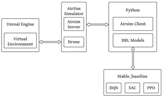
Figure 1.
System architecture of this study.
3.2. Reinforcement Learning
The concept of reinforcement learning pertains to a method of dynamic programming through which algorithms are taught using rewarding and punishing systems. Through trial and error, RL-based techniques help drone agents gain experience in simulated environments. The objective is to give an agent the freedom to navigate around the environment, engage with the environment, and use the rewards it receives for each action it performs to improve the policy. Reinforcement learning is defined by five main components: environment, agent, state, action, and rewards. An illustration of the reinforcement learning block diagram is shown in Figure 2. The following subsections explore each component in detail.
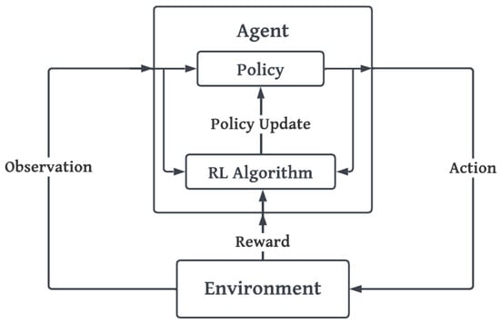
Figure 2.
Main components of reinforcement learning.
3.2.1. Environment
The central element of the reinforcement learning problem is the environment. It is the world that exists outside the agent where the agent (drone) operates. The environment receives the agent’s present state and action as inputs and returns the agent’s reward and the subsequent state as outputs. This research aims to train the drone to identify obstacles and avoid colliding with them. For effective collision avoidance, the gap between the real and training environments should be minimal. This means that the environment should closely resemble the real world. The environment should be designed in such a way that it assists in training the drone to reach the target location while detecting and avoiding collisions.
For this research, the environment is built in Unreal Engine 4 and the drone is provided by AirSim. Aerial Informatics and Robotics Simulation, or AirSim, is an open-source, cross-platform drone and ground vehicle simulator. The plugin is designed to be an accessory for Unreal and can be dropped into any Unreal game environment to enable the feature. Unreal 4 offers a variety of drawing tool libraries, which were used to construct three distinct environments for training and testing the drone.
Training Environment
Figure 3 provides snapshots of the training environments. All the environments have four walls and just one exit. The drone must find its way out of the room without colliding with any obstacles. The first environment is called the obstacle world, which is a closed chamber packed with various shapes and objects. The second one, called the woodland world, mimics a forest setting with trees of varying sizes and branch varieties. The third environment is a dynamic oscillatory world made up of objects in various shapes that move in different directions, along with individuals walking and dancing.
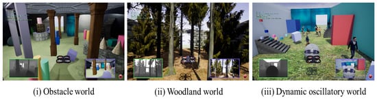
Figure 3.
Training environment for the drone.
Testing Environment
Figure 4 provides snapshots of the testing environments. The testing environments will be used to find out which of the three proposed algorithms is the most efficient. Two different environments are created. The first environment is a simple, enclosed room with tall pillars. In the second environment, the complex world, there is an increase in difficulty because of the presence of trees, people walking, and other dynamic objects.
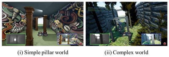
Figure 4.
Testing environment for the drone.
3.2.2. State
The circumstance that an agent is in at any given time is known as its state. It is the set of information an agent knows about its environment at a given time. The state is crucial to reinforcement learning because it enables the agent to analyze its progress and make decisions based on previous experience. The state helps the agent plan its forthcoming controls based on its goals and current situation. The front camera image from the drone is used in determining the state. The image is retrieved by AirSim, which provides RGB and depth images of the environment as shown in Figure 5. The project uses depth images as the state since they are insensitive to color illumination, rotation angle, and scale changes.
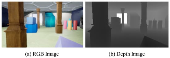
Figure 5.
Images obtained from drone camera.
3.2.3. Actions
Agents can shift between states by interacting with and altering their environment through the use of actions. Every action the agent takes results in a reward from the environment. The policy determines the next action based on the rewards. An agent’s permissible actions in a given environment are referred to as its action space. Each environment has a unique action space linked to it. Two kinds of activity spaces are used in this research. Figure 6 depicts the discrete action space, which consists of five actions: move forward, move backward, move left, move right, and idle. In continuous action space, the above five actions are performed by generating a real value vector of length two. The actions only influence the drone’s x and y axes. Limiting the drone’s movement to only the x and y axes while keeping the z-axis constant enables the training process to be more targeted and effective. For the drone to be able to encounter all obstacles on the course, it is positioned closer to the ground. When the dimensionality of the problem is reduced, it becomes easier to design and test autonomous navigation algorithms, resulting in a faster and more efficient training process.
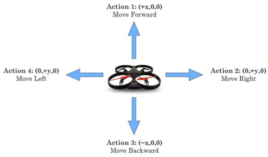
Figure 6.
Action space of drone.
3.2.4. Rewards
Rewards are the feedback the agent receives based on the action it performed. Over the course of an episode, the agent’s objective is to maximize its total reward. Rewards drive the agent to behave in a particular way. All actions result in feedback, which may be positive (reward) or negative (punishment), depending on whether the action was desired or not. The reward function for different states is given in Table 1. The highest reward is awarded when the drone reaches its goal. The lowest is when a collision occurs. Both cases result in the current episode terminating and a new one beginning. In order to motivate the drone to reach its goal, its reward is based on the distance traveled from its old state to the new state. The reward is positive if the goal is closer than before; otherwise, a negative reward is given.

Table 1.
Reward functions.
3.2.5. Agent
An agent is the learner and decision-maker of a reinforcement learning model. Reinforcement learning objective is to teach the agent how to complete a specific task in an environment of uncertainty. The agent consists of two components: policy and learning algorithm, which work together to maximize rewards. The policy maps the currently observed environment to a probability distribution of the actions that will be executed. A function approximator with configurable parameters and a particular approximation model, such as a deep neural network, is used by an agent to carry out the policy. The learning algorithm adjusts the policy settings continuously based on actions, observations, and incentives. The learning algorithm looks for the best course of action to take in order to maximize the projected long-term cumulative reward from the activity.
3.3. Deep Convolutional Neural Network in RL Policy
A policy defines a way for mapping an agent’s state to actions. Policies are made up of several networks that coordinate with associated optimizers. Each of these networks has a feature extractor followed by a fully-connected network. There are various layers of neural networks that make up the Deep Convolutional Neural Network (DCCN). DCCNs are chosen because of their efficiency, ability to extract features from image input, and ability to map them to appropriate actions. In contrast to other neural network architectures, such as Multi-Layer Perceptron (MLP) or Recurrent Neural Networks (RNN), CNN can capture local and global patterns in images using convolutional and pooling layers. The design of CNN allows embedding specific features into the architecture for image inputs. These greatly decrease the number of parameters in the network and enhance the implementation efficiency of the forward function.
The architecture of CNN used in the policy network is shown in Figure 7. In the architecture, the layers are alternated by RELU activation functions, which improve the optimization process by accelerating the convergence rate. A common problem in neural network training is overfitting, but RELU activation functions are computationally efficient and reduce this risk. The depth image collected from the drone is rescaled to size 84 × 84 and fed to the CNN network as input data. This reduces the dimensionality of the input image, which lowers the number of parameters in the network and increases forward function efficiency. Throughout the training process, the filter matrix will constantly update itself to determine a reasonable weight. The last layer is a fully connected neural network with 512 hidden nodes. The final output indicates the next action to take. The dimensions of the architecture are given in Table 2.
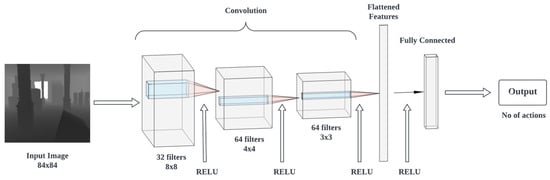
Figure 7.
CNN Architecture of the policy.
Table 2.
Summary of CNN architecture.
3.4. Reinforcement Learning Algorithms
3.4.1. Deep Q-Networks (DQN)
The Deep Q-network (DQN) algorithm is a model-free, off-policy reinforcement learning method. It is one of the first algorithms to incorporate deep neural networks into reinforcement learning. The implementation of deep neural networks in reinforcement learning has previously been unsuccessful due to their instability. It is difficult to generalize deep neural networks in reinforcement learning models because they are prone to overfitting. DQN algorithms address this problem by providing diverse and de-correlated training data. This is done by storing all the experiences of the agent, and randomly sampling and replaying those experiences [22]. In the DQN algorithm, actions are learned by Q-learning, and the Q-value function is estimated using a deep neural network. Q-learning is an off-policy RL algorithm. In its most basic form, it employs a table to keep track of all Q-values for all prospective state-action combinations. The Bellman equation is used to update this table, and the action is mostly chosen using an ε-greedy policy. The link between a certain state (or state-action pair) and its successor is described by the Bellman equation. The recursive form of the Q-function is given as in Equation (1).
where
- —Q-value of step
- —reward received
- —discount factor in range [0,1]
The optimal value of Q is achieved by selecting the action that will yield the highest return as shown in Equation (2). Since there are no further rewards after the episode’s final step, the Q-function is equal to the last reward, hence Equation (1) is altered to truncate the last Q-value and a flag called done is introduced. The goal is to gradually converge the current Q-value to the optimal value of Q.
where
- —optimal Q-value of state and action
- —immediate reward received
- —discount factor in range [0,1]
- —done flag, which is 1 for last step, otherwise 0
- —maximum Q-value obtained for state for action
The DQN architecture consists of two neural nets, the Q-network and the target network, and an experience replay component as depicted in Figure 8. The Q-network is the trained agent for determining the optimal state-action value. In terms of structure, the target network is exactly the same as the Q-network. DQN estimates the target and prediction Q-values using two independent networks with the same design in order for the Q-learning algorithm to be stable. Weights in the Q-network are updated after each iteration, but those in the target network are not updated until N iterations have passed. The results from the target network are used as ground truth for Q-network.
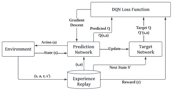
Figure 8.
Architecture of DQN model.
This study follows a CNN architecture for Q-network and target network as shown in Figure 7. The loss function calculates the error and assists in optimizing the weights thereby minimizing error during the learning process. Loss is computed based on the predicted Q-value, target Q-value, and observed reward for the data sample as given in Equation (3).
where
- —predicted Q-value
- —target Q-value
- —trainable weights of the network
The Q-learning process oscillates or diverges with the neural network process. As the policy changes or oscillates rapidly with slight changes to the Q-value, the distribution of data can shift from one extreme to another. To solve the above problem, transitions are stored in a replay buffer, and a small sample of recorded experience is used to update the Q-network [23]. With experience replay, successive correlations between samples will be broken, and the network will be better able to utilize the experiences. The working of the DQN model is summarized in Algorithm 1.
| Algorithm 1: Deep Q-Learning | ||
| Initialize prediction network and target network Initialize experience replay buffer For episode = 1 to | ||
| For step = 1 to | ||
| Choose action according to -greedy policy given as Move drone from state based on action , and get the reward and next state Store the transition (, , , , ) in Generate a random minibatch sample of transitions (, , , , ) from Apply stochastic gradient descent to update with respect to the network parameters using calculated loss Copy weights from to for every C steps | ||
| End For | ||
| End For | ||
3.4.2. Proximal Policy Optimization (PPO)
The Proximal Policy Optimization (PPO) method is an on-policy, policy gradient reinforcement learning approach. The PPO algorithm is inspired by A2C to have multiple workers and by TRPO to use a trust region to improve the actor. A key idea here is to ensure that following a policy update, the new policy does not deviate significantly from the old policy. PPO employs clipping in such situations to prevent updates that are too large. This algorithm samples data based on the environmental interaction and a clipped surrogate loss function is optimized using stochastic gradient descent. The action space can be either discrete or continuous.
An outline of the PPO architecture can be seen in Figure 9. An actor-critic approach is used by the agent, which uses two CNN models, one called Actor, and one called Critic. PPO follows an on-policy learning approach. The decision-making policy is updated based on a small sample of experience gathered from the environmental interaction. The experiences are discarded when this batch of experiences is used to update the policy, and a fresh set is gathered using the most current policy revision. The policy parameter is updated based on the clipped loss function given in Equation (4). The loss function contains a hyperparameter that tells how far the revised policy should deviate from the old policy.
where
- —probability ratio
- —advantage function
- —hyperparameter

Figure 9.
Architecture of PPO model.
The clipped loss function computes the probability ratio between the current policy and the old policy as given in Equation (5). When , the action is selected more in the current policy and when , the action will be selected less in the current policy.
where
- —current policy
- —old policy
The advantage function is the difference between the value function of the policy and the future discounted summation of rewards for the given state and action as given in Equation (6). The advantage function indicates how much effective an action would be relative to the return based on an average action. When the variation in gradient estimates between the old and new policy is decreased, the RL algorithm becomes more stable.
where
- —state-value function for state
- —reward for step
- —discount factor
The state-value function assesses how favorable the circumstances are in a state. The equation of state-value function is given as Equation (7).
where —Q-value/action-value of state and action for parameter .
The advantage function indicates if a state is better or worse than anticipated. Figure 10 visualizes the clipped loss function based on the advantage [24]. The advantage is positive when the current action is more favorable than the previous one. After the threshold, , the current action plan becomes too favorable, and taking such a large amount of change into account increases variance and reduces consistency. To prevent the policy function from updating too much if the action is too successful, the clipped version of the graph has a flat line once the ratio function increases larger than . When an action results in a negative advantage, it signifies that the current action is not much better than the prior one and that it will attempt to lower the ratio function below 1. However, lowering the ratio function too much will result in a significant change, thus it is clipped to be higher than . The loss function of the critic network is defined as the mean squared loss with the returns as given in Equation (8). A summary of the overall functioning of the PPO model is given in Algorithm 2.
where
- —state-value function of critic network
- —discounted sum of future rewards in the trajectory as given in Equation (9)
- —discount factor for the step
- —reward for the step

Figure 10.
Clipped loss with reference to probability ratio for positive and negative advantages.
| Algorithm 2: Proximal Policy Optimization | |
| Initialize initial policy parameters for actor network Initialize initial value function parameters for critic network For k = 0, 1, 2, … | |
| Run the policy in the environment to gather a set of trajectories taken by the drone Obtain the reward and compute rewards-to-go Calculate advantage estimates based on current value function Apply stochastic gradient ascent with Adam to update the policy with respect to the network parameters by maximizing the clipped loss Update the critic’s parameter by stochastic gradient descent on loss function | |
| End For | |
3.4.3. Soft Actor-Critic (SAC)
Many on-policy algorithms suffer from sample inefficiency because they are required to collect new samples each time the policy is updated, resulting in lower efficiency. In contrast, Q-learning-based off-policy algorithms can efficiently learn from past samples using experience of replay buffers, but a lot of tuning is necessary because these algorithms are very hyperparameter sensitive. The soft actor-critic (SAC) algorithm is a model-free, off-policy, actor-critic reinforcement learning method. A prominent feature of SAC is that it uses a modified RL objective function. Consequently, SAC focuses on maximizing not only lifetime rewards but also the entropy of the policy. Policy entropy measures the level of uncertainty based on the present state. The higher the entropy value, the more exploration will take place. To balance exploration and exploitation of the environment, it is imperative to maximize both the reward and the entropy. The entropy for policy is calculated as shown in Equation (10):
where —stochastic policy.
In entropy-regularized reinforcement learning, the agent receives bonuses at each step based on the policy entropy at that instant. Thus, the RL problem becomes as shown in Equation (11).
where
- —reward obtained for action at state
- —discounted factor
- —entropy of the policy
- —trade-off coefficient
The architecture of SAC is drawn in Figure 11. SAC agent uses both actor and critic networks. For a given state and action, the critic returns the estimated discounted value of the cumulative long-term reward, whereas an actor returns the action that maximizes the discounted value. The actor employs a policy gradient technique during training and learns more about the best course of action by examining critics’ feedback rather than just focusing on the rewards. Similar to how the actor learns through rewards, the critic advances in a value-based approach so that it can critique the actor effectively in the future. As part of its design, SAC consists of three networks: a soft Q-function parameterized by , a state-value function parameterized by , and a policy function parameterized by . The soft Q-value and soft state-value of the SAC model are given in Equations (12) and (13).
where
- —reward obtained for action at state
- —discounted factor
- —stochastic policy
- —state distribution induced by the policy

Figure 11.
Architecture of SAC model.
Although in theory the and functions, which are related by the policy, do not need separate approximators, having separate approximators aids in convergence [25]. Taking this into account, we will need to train three approximators for each function as follows:
Learning of the State-Value Function
The state-value function, denoted by , is a function that estimates the expected future return of being in state S while following the current policy. The state-value function is learned by minimizing the squared residual error , as shown below in Equation (14):
where
- —experience replay buffer
- —trade-off coefficient
In order to update the parameters of the V-function, the approximation of the derivative of the objective is used in Equation (15):
Learning of the Q-Function
The soft Q-function, denoted by , is a function that estimates the expected future return of taking action in state , while following the current policy. The Q-function is updated by minimizing the mean squared error between the Q-values and the target Q-values. The Q-function loss is given by Equation (16):
where
- —target value function parameterized by
- —discounted factor
The parameters of is updated using the approximation of the derivative of the objective , which is given in Equation (17):
Learning of the Policy
The policy, denoted by π(s), is a function that maps states to actions. The goal of the algorithm is to find the optimal policy that maximizes the expected future return. In SAC, the policy is defined as a stochastic policy with a parameterized probability. The loss function of the policy is given in Equation (18). A neural network transformation is utilized to reparametrize in the loss function and ensure that sampling from the policy has a differentiable component.
where
- —input noise vector sampled from Gaussian distribution
- —reparametrized variable which evaluates action
In order to update the parameters of the policy function, the approximation of the derivative of the objective is used in Equation (19):
Furthermore, SAC stores and samples experiences randomly in a replay buffer during training, which improves sample efficiency and reduces the correlation between samples. The overall working of the SAC model is summarized in Algorithm 3.
| Algorithm 3: Soft Actor-Critic | |||
| Initialize prediction network , target network , and policy network Initialize policy for the three networks , and , respectively Initialize experience replay memory For step = 1, 2, 3, … | |||
| Observe state and select action Move drone based on action , and get the reward , next state and done signal Store the transition (, , , , ) in If is terminal i.e., is 1 | |||
| Reset environment state | |||
| Else | |||
| Generate a random minibatch sample of transitions (, , , , ) from For every transition in minibatch | |||
| Update the Q-function by one step of gradient descent using Update the policy by maximizing Update the value function by applying gradient descent using | |||
| End For | |||
| End If | |||
| End For after convergence | |||
4. Experimental Results
4.1. Training Evaluation
This work attempts to train the drone to avoid collisions on its own by detecting and avoiding obstacles autonomously. A reinforcement learning approach was employed to achieve this goal, and three different algorithms were compared to find the most effective one. Several environments varying in difficulty were used to train the algorithms, as shown in Figure 3, which have been characterized by different levels of difficulty. The goal is to get to the exit point without hitting any obstacles. Based on the actions taken by the drone, both positive and negative rewards were assigned to it. The algorithms were trained for 100 k steps. Every time an episode started, the environments were chosen randomly and drones were placed in different starting points to increase randomness.
During the training process, the algorithms were evaluated every 500 steps to analyze the performance. The evaluation results of three algorithms—DQN, PPO, SAC—are provided in Figure 12, Figure 13 and Figure 14, respectively. The mean rewards of all three algorithms appear to increase as the number of training steps increases, which suggests that the training is progressing in the right direction. SAC seems to have the highest reward owing to its actor-critic architecture and sample-efficient characteristics. SAC employs entropy regularization in order to maximize the trade-off between expected return and entropy (randomness in the policy). Contrary to popular belief, DQN outperformed PPO in this case. This is because DQN offers better sample efficiency via the replay buffer. The PPO policies are prone to overshooting and miss the reward peak or stall prematurely when the policy updates are made. Especially in neural network architectures, vanishing and exploding gradients are one of the most challenging aspects. There is a possibility that the algorithm may not be able to recover from a poor update.
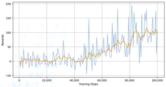
Figure 12.
Training evaluation of DQN.
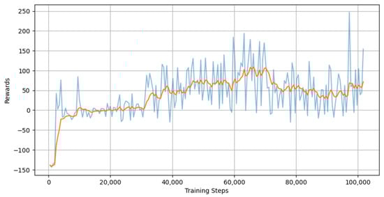
Figure 13.
Training evaluation of PPO.
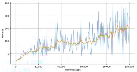
Figure 14.
Training evaluation of SAC.
4.2. Case Studies
To better understand and verify the effectiveness of the three algorithms, several tests are designed to study the behavior. Two different testing environments were created in Unreal Engine 4 where the trained models were tested. The case studies discuss how different algorithms were able to get to the desired goal, and how long it took them to accomplish it.
4.2.1. Case-1: Simple Pillar World
In this case study, the environment is set in a closed room with pillars positioned at random locations throughout the room. A snapshot of the environment is given in Figure 4i. A diagram illustrating the position of the pillars can be found in Figure 15b. The simulation results are given in Figure 15, which visualizes the time and path taken by the different algorithms in the simple pillar world. Based on the results, we conclude that DQN and SAC successfully made it to the exit without any collisions. DQN even managed to reach the exit before SAC as shown in Figure 15a. In Figure 15b, it is visible that PPO took a slight detour, possibly hitting the wall in the process, thus ending the episode. Likewise, SAC also had close contact with the wall but was able to turn back just in time and avoid hitting it. The models seemed to have all taken a path that was inclined to the right at first. This is because most of the pillars appear to be on the left side, which means the models were able to choose a path with the fewest obstacles.
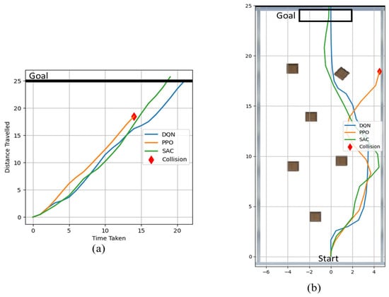
Figure 15.
Results from Case-1: (a) time taken to reach the goal; (b) the path taken by the algorithm.
4.2.2. Case-2: Complex World with Moving Obstacles
This case study envisions an environment with an open-roof room. Most of the room is surrounded by trees on all sides. A snapshot of the environment is given in Figure 4ii. As part of this case study, two mobile obstacles have been introduced: an archer walking and a ball rolling. Figure 16b shows an illustration of how different obstacles are positioned relative to one another in the environment. The figure also depicts the trajectory of the mobile obstacles. The simulation results are given in Figure 16, which visualizes the time and path taken by different algorithms. It is interesting to note that all algorithms managed to reach the exit even though it seems to be a more complex environment than Case-1. As seen from the time graph in Figure 16a, SAC and PPO reached the exit at about the same time. In addition, Figure 16b reveals that PPO took an unnecessary zigzag path toward the end and still managed to reach the exit along with SAC.
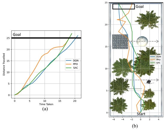
Figure 16.
Results from Case-2: (a) time taken to reach the goal; (b) the path taken by the algorithm.
4.3. Discussion
A comparative study of three different algorithms—DQN, PPO, and SAC—was conducted for obstacle detection and avoidance in UAVs, including the analysis of their strengths, weaknesses, and trade-offs. The evaluation results showed that for all three algorithms, mean rewards increased as the number of training steps increased, indicating progress in the right direction. SAC performed the best among the three algorithms because of its actor-critic architecture and sample-efficient characteristics. PPO performed poorly among the algorithms, suggesting that on-policy algorithms are not suitable for effective collision avoidance in large 3D environments with dynamic actors. Off-policy algorithms, DQN and SAC, returned promising results. DQN outperformed PPO due to its better sample efficiency via the replay buffer. In the testing phase, the obstacles in the testing environments were kept at a reasonable distance from one another. In small paths and turns, DQN might not be as advantageous due to its restricted discrete action space.
A further evaluation of the three algorithms was conducted in different environments in order to verify their effectiveness. In Case-1, both DQN and SAC successfully made it to the exit without any collisions, while PPO took a slight detour, possibly hitting the wall in the process. In Case-2, all algorithms managed to reach the exit even though it was a more complex environment than in Case-1. Overall, the experimental results indicate that reinforcement learning using SAC and DQN algorithms can efficiently train a drone to detect and avoid obstacles autonomously in varying environments. Moreover, PPO models tend to follow zigzag paths, possibly because they tend to take sharp angles in their actions. This led them to reach the destination slower in Case-2. While it may be possible to incorporate constraints that limit sharp turns, this approach has limitations as it may compromise the adaptability and flexibility of the RL model and introduce biases that are not representative of the real-world environment. Such constraints may also result in suboptimal policies that are not adaptable to new situations. Instead, training the model in diverse environments can enable it to learn to navigate to different coordinates using a range of methods. The drone can benefit from this training method by acquiring a more generalized policy and improving its ability to adjust to environmental changes.
5. Conclusions and Future Work
This work aims to develop a drone that can operate autonomously. The use of automated drone systems increases productivity by removing the need for drone operators and enabling reliable real-time data to be accessed more conveniently. The advantages and opportunities of autonomous drones are numerous. However, one of the most challenging aspects of autonomous drones is the detection and avoidance of collisions. The paper compares three different reinforcement learning approaches that could aid in effectively avoiding stationary and moving obstacles. The study was conducted in a simulated setting by AirSim, which provides realistic environments for testing autonomous systems without risking damage to expensive hardware or endangering human lives. Different training and testing environments were created using Unreal Engine 4. The comparison of the three different algorithms revealed that SAC performed the best, followed by DQN, while PPO was found to be unsuitable for large 3D environments with dynamic actors. Overall, off-policy algorithms are more efficient in avoiding collisions than on-policy algorithms. The proposed approach can be applied to different types of UAVs and environments by training the deep reinforcement learning algorithm on diverse datasets.
In future research, the effectiveness of the collision avoidance algorithms could be improved by training them in more environments that mimic the real world. The research could be extended to creating a path-following model, which would be incorporated into the current model. It would also be worthwhile to assess the hardware power consumption and other related factors, as well as its efficiency in real-life situations by incorporating it into a real drone and analyzing how it avoids obstacles.
Author Contributions
Conceptualization, A.P.K., C.J.J. and A.Q.M.; data curation, C.J.J.; funding acquisition, S.B.; investigation, A.Q.M., S.B. and S.M.; methodology, A.P.K., S.B., S.M. and S.S.; project administration, A.Q.M.; software, A.P.K. and C.J.J.; supervision, S.B., S.M. and S.S.; validation, S.S.; writing—original draft, A.P.K. and C.J.J.; writing—review and editing, A.Q.M., S.M. and S.S. All authors have read and agreed to the published version of the manuscript.
Funding
Princess Nourah bint Abdulrahman University Researchers Supporting Project number (PNURSP2023R195), Princess Nourah bint Abdulrahman University, Riyadh, Saudi Arabia.
Institutional Review Board Statement
Not applicable.
Informed Consent Statement
Not applicable.
Data Availability Statement
Not applicable.
Acknowledgments
This research is supported by Princess Nourah bint Abdulrahman University Researchers Supporting Project number (PNURSP2023R195), Princess Nourah bint Abdulrahman University, Riyadh, Saudi Arabia.
Conflicts of Interest
The authors have no competing interests to declare that are relevant to the content of this article.
Abbreviations
The following abbreviations are used in this manuscript:
| 3DVFH | 3-Dimensional Vector Field Histogram |
| A2C | Advantage Actor-Critic |
| ACKTR | Actor-Critic using Kronecker-factored Trust Region |
| CNN | Convolutional Neural Network |
| DD-DQN | Dueling Double Deep Q-Network |
| DNN | Deep Neural Network |
| DQN | Deep Q-Network |
| PID | Proportional Integral Derivative |
| PPO | Proximal Policy Optimization |
| RELU | Rectified Linear Unit |
| ResNet | Residual Network |
| RL | Reinforcement Learning |
| SAC | Soft Actor Critic |
| SIFT | Scale Invariant Feature Transform |
| SURF | Speeded Up Robust Features |
| SVM | Support Vector Machine |
| TRPO | Trust Region Policy Optimization |
| UAV | Unmanned Aerial Vehicle |
| VAE | Variational Autoencoders |
| VREP | Virtual Robot Experimentation Platform |
| YOLO | You Only Look Once |
References
- Chaturvedi, S.K.; Sekhar, R.; Banerjee, S.; Kamel, H. Comparative Review Study of Military and Civilian Unmanned Aerial Vehicles (UAVs). INCAS Bull. 2019, 11, 183–198. [Google Scholar] [CrossRef]
- Fan, J.; Saadeghvaziri, M. Applications of Drones in Infrastructures: Challenges and Opportunities. Int. J. Mech. Mechatron. Eng. 2019, 13, 649–655. [Google Scholar] [CrossRef]
- Mohsan, S.A.H.; Khan, M.A.; Noor, F.; Ullah, I.; Alsharif, M.H. Towards the Unmanned Aerial Vehicles (UAVs): A Comprehensive Review. Drones 2022, 6, 147. [Google Scholar] [CrossRef]
- AlMahamid, F.; Grolinger, K. Autonomous Unmanned Aerial Vehicle navigation using Reinforcement Learning: A systematic review. Eng. Appl. Artif. Intell. 2022, 115, 105321. [Google Scholar] [CrossRef]
- Kan, M.K.; Okamoto, S.; Lee, J.H. Development of drone capable of autonomous flight using GPS. In Proceedings of the International MultiConference of Engineers and Computer Scientists Vol II, Hong Kong, China, 14–16 March 2018. [Google Scholar]
- Kanellakis, C.; Nikolakopoulos, G. Survey on Computer Vision for UAVs: Current Developments and Trends. J. Intell. Robot Syst. 2017, 87, 141–168. [Google Scholar] [CrossRef]
- Xue, Z.; Gonsalves, T. Vision Based Drone Obstacle Avoidance by Deep Reinforcement Learning. AI 2021, 2, 366–380. [Google Scholar] [CrossRef]
- Al-Kaff, A.; García, F.; Martín, D.; de La Escalera, A.; Armingol, J. Obstacle Detection and Avoidance System Based on Monocular Camera and Size Expansion Algorithm for UAVs. Sensors 2017, 17, 1061. [Google Scholar] [CrossRef] [PubMed]
- Aldao, E.; González-deSantos, L.M.; Michinel, H.; González-Jorge, H. UAV Obstacle Avoidance Algorithm to Navigate in Dynamic Building Environments. Drones 2022, 6, 16. [Google Scholar] [CrossRef]
- Shin, S.-Y.; Kang, Y.-W.; Kim, Y.-G. Obstacle Avoidance Drone by Deep Reinforcement Learning and Its Racing with Human Pilot. Appl. Sci. 2019, 9, 5571. [Google Scholar] [CrossRef]
- Martins, W.M.; Braga, R.G.; Ramos, A.C.B.; Mora-Camino, F. A Computer Vision Based Algorithm for Obstacle Avoidance. In Information Technology—New Generations; Springer International Publishing: New York, NY, USA, 2018; pp. 569–575. [Google Scholar] [CrossRef]
- Sarmalkar, K.; Jain, S.; Hangal, S. Vision based Obstacle Avoidance System for Autonomous Aerial Systems, NTASU 2020. IJERT 2021, 9, 730–734. Available online: www.ijert.org (accessed on 10 January 2023).
- Guo, J.; Liang, C.; Wang, K.; Sang, B.; Wu, Y. Three-Dimensional Autonomous Obstacle Avoidance Algorithm for UAV Based on Circular Arc Trajectory. Int. J. Aerosp. Eng. 2021, 2021, 1–13. [Google Scholar] [CrossRef]
- Aswini, N.; Uma, S.V. Obstacle Detection in Drones Using Computer Vision Algorithm. In Communications in Computer and Information Science; Springer: Berlin/Heidelberg, Germany, 2019; Volume 968, pp. 104–114. [Google Scholar] [CrossRef]
- Mori, T.; Scherer, S. First results in detecting and avoiding frontal obstacles from a monocular camera for micro unmanned aerial vehicles. In Proceedings of the 2013 IEEE International Conference on Robotics and Automation, Karlsruhe, Germany, 6–10 May 2013; pp. 1750–1757. [Google Scholar] [CrossRef]
- Mannar, S.; Thummalapeta, M.; Saksena, S.K.; Omkar, S. Vision-based Control for Aerial Obstacle Avoidance in Forest Environments. IFAC-PapersOnLine 2018, 51, 480–485. [Google Scholar] [CrossRef]
- Zhai, X.; Liu, K.; Nash, W.; Castineira, D. Smart Autopilot Drone System for Surface Surveillance and Anomaly Detection via Customizable Deep Neural Network. In Proceedings of the International Petroleum Technology Conference, Dhahran, Saudi Arabia, 13–15 January 2020. [Google Scholar] [CrossRef]
- Fang, R.; Cai, C. Computer vision based obstacle detection and target tracking for autonomous vehicles. MATEC Web Conf. 2021, 336, 07004. [Google Scholar] [CrossRef]
- Yang, S.; Meng, Z.; Chen, X.; Xie, R. Real-time obstacle avoidance with deep reinforcement learning Three-Dimensional Autonomous Obstacle Avoidance for UAV. In Proceedings of the 2019 International Conference on Robotics, Intelligent Control and Artificial Intelligence—RICAI 2019, Shanghai, China, 20–22 September 2019; pp. 324–329. [Google Scholar] [CrossRef]
- Roghair, J.; Niaraki, A.; Ko, K.; Jannesari, A. A Vision Based Deep Reinforcement Learning Algorithm for UAV Obstacle Avoidance. In Intelligent Systems and Applications; Springer: Berlin/Heidelberg, Germany, 2022; Volume 294, pp. 115–128. [Google Scholar] [CrossRef]
- Rubí, B.; Morcego, B.; Pérez, R. Quadrotor Path Following and Reactive Obstacle Avoidance with Deep Reinforcement Learning. J. Intell. Robot Syst. 2021, 103, 62. [Google Scholar] [CrossRef]
- Mnih, V.; Kavukcuoglu, K.; Silver, D.; Rusu, A.A.; Veness, J.; Bellemare, M.G.; Graves, A.; Riedmiller, M.; Fidjeland, A.K.; Ostrovski, G.; et al. Human-level control through deep reinforcement learning. Nature 2015, 518, 529–533. [Google Scholar] [CrossRef] [PubMed]
- Mnih, V.; Kavukcuoglu, K.; Silver, D.; Graves, A.; Antonoglou, I.; Wierstra, D.; Riedmiller, M. Playing Atari with Deep Reinforcement Learning. arXiv 2013, preprint. arXiv:1312.5602. [Google Scholar]
- Schulman, J.; Wolski, F.; Dhariwal, P.; Radford, A.; Klimov, O. Proximal Policy Optimization Algorithms. arXiv 2017, arXiv:1707.06347. [Google Scholar]
- Haarnoja, T.; Zhou, A.; Abbeel, P.; Levine, S. Soft Actor-Critic: Off-Policy Maximum Entropy Deep Reinforcement Learning with a Stochastic Actor. 2018. Available online: https://proceedings.mlr.press/v80/haarnoja18b/haarnoja18b.pdf (accessed on 12 January 2023).
Disclaimer/Publisher’s Note: The statements, opinions and data contained in all publications are solely those of the individual author(s) and contributor(s) and not of MDPI and/or the editor(s). MDPI and/or the editor(s) disclaim responsibility for any injury to people or property resulting from any ideas, methods, instructions or products referred to in the content. |
© 2023 by the authors. Licensee MDPI, Basel, Switzerland. This article is an open access article distributed under the terms and conditions of the Creative Commons Attribution (CC BY) license (https://creativecommons.org/licenses/by/4.0/).