Abstract
Rapidly completing the exploration and construction of unknown environments is an important task of a UAV cluster. However, the formulation of an online autonomous exploration strategy based on a real-time detection map is still a problem that needs to be discussed and optimized. In this paper, we propose a distributed unknown environment exploration framework for a UAV cluster that comprehensively considers the path and terminal state gain, which is called the Distributed Next-Best-Path and Terminal (DNBPT) method. This method calculates the gain by comprehensively calculating the new exploration grid brought by the exploration path and the guidance of the terminal state to the unexplored area to guide the UAV’s next decision. We propose a suitable multistep selective sampling method and an improved Discrete Binary Particle Swarm Optimization algorithm for path optimization. The simulation results show that the DNBPT can realize rapid exploration under high coverage conditions in multiple scenes.
1. Introduction
At present, unmanned aerial vehicles (UAVs) are widely used to perform tasks in various environments, especially in complex and unknown scenes. One of the typical tasks is to explore an unknown environment, which is widely used for search [1,2], rescue [3,4], and dangerous area reconnaissance [5]. Unknown environment exploration means that UAVs or a UAV cluster can make decisions on their own actions in real-time by relying on their detection equipment under the condition that there is no prior environmental information to achieve a fully independent construction of highly saturated environmental information. Compared with other missions, unknown environment exploration lacks prior map information. It is crucial to set the autonomous strategy of the exploration action to complete the environmental construction of the whole region as soon as possible. The coordination in the cluster and avoidance of repeated exploration must also be considered.
The traditional exploration of unknown environments adopts the ploughing method for complete coverage path planning [6], but it only aims at specific conditions [7] without obstacles in the environment. When encountering obstacles, the ploughing method adopts a simple wall-following strategy [8] to avoid sudden obstacles in the path, which also has great limitations. Yamauchi initiated a frontier-based exploration strategy [9] and extended it to multiple robots [10], which is considered to be an important classical method for unknown environment exploration. The frontier is defined as the boundary between the unexplored grid and the explored grid while excluding the explored obstacle grid. The frontier-based method obtains exploration information by navigating the robot to the frontier grid. Many of the most advanced methods are based on frontier-based exploration [11,12,13]. Ref. [14] developed a frontier-selection strategy that minimizes the change in velocity necessary to reach it to achieve the high-speed movement of quadrotors. Ref. [15] proposed a hierarchical planning framework based on frontier information (FIS), enabling a UAV cluster to quickly explore indoor environments.
The sampling-based method is another particularly effective method for exploration. The central idea is to calculate the information gain of the sampled state and select the best one to execute, which can adapt to various gain calculation forms and has strong flexibility. The sampling-based method is also combined well with the frontier-based method. For example, the SRT [16] algorithm drives the motion update of the robot through sampling in the sensor safety space and the selection of random exploration angles. The Next-Best-View (NBV) [17,18] is an exploration method introduced from 3D reconstruction and has become a widely used sample-based exploration method. Authors in [19] proposed the Receding Horizon Next-Best-View, combining NBV with a path planning algorithm similar to RRT [20] and RRT* [21], and obtained a fine effect in indoor exploration and reconstruction mapping. Authors in [22] proposed a UFO exploration method. Based on the rapidly updated map format called the UFO Map, the maximum information gain was not considered but adopted the nearest point with the information gain as the exploration decision, which achieved the effect of rapid exploration at a small cost of computing resources. In addition, exploration methods based on machine learning are also considered to have great potential, and many scholars are conducting relevant research [23,24,25]. However, its engineering applications for unknown environment exploration are still relatively few, and it performs poorly in the generalization ability to different environments, which still needs further exploration and research [26,27].
For large scenes, such as in underground garages or large factories, to ensure that the task can be completed quickly, the cluster is generally used. For the exploration of the environment of a robot cluster, the distributed cluster structure is considered to be better in this scenario [28]. It can not only avoid excessive pressure on central computing resources but also flexibly handle the impact of poor communication in the cluster or sudden failures [29,30,31] to minimize efficiency loss. However, for distributed clusters, designing the exploration strategy of each platform to avoid repeated exploration and complete the exploration quickly under the premise of cluster collision avoidance is still a difficult problem.
The above method seems to simply consider the state of the next step to calculate its gain, but the impact of its motion process on the exploration is considered to be negligible, especially when the sensor is limited by the field of view (FOV) or is in the area near the obstacle, and at the same time, dynamics should be considered to increase the efficiency. Therefore, this paper proposes a distributed exploration framework for unknown environments considering the path and terminal gain. In this framework, multiple exploration paths are obtained by considering the dynamic constraints of the state sequence, and the optimal path is obtained by using optimization methods. The evaluation factors include the energy loss of dynamics, the growth of map exploration in the path process, the benefits of the terminal state to the next exploration, and collision avoidance in the cluster. The paths are planned for a period of time in the future and take the frontmost path to implement until the exploration coverage of the entire cluster meets the requirements. To ensure the efficiency of online planning, a multistep selective optimal sampling method, a gain calculation method of path exploration, and an efficient improved Discrete Binary Particle Swarm Optimization (BPSO) algorithm are given. The results show the effectiveness and superiority of the algorithm in the exploration of unknown environments of a UAV cluster in multiple scenes.
The contributions of this paper are as follows:
- A Distributed Next-Best-Path and Terminal framework for real-time path planning for UAV cluster unknown environment exploration.
- A multistep selective sampling method for the initial generation of the exploration path with the calculation method of progress and terminal gain.
- An improved Discrete Binary Particle Swarm Optimization algorithm to generate the best exploration path.
The remainder of this paper is organized as follows: Section 2 describes the problem of unknown environment exploration and introduces our distributed unknown environment exploration framework and the construction of the specific model. Section 3 discusses the multistep selective sampling method we propose and the improved BPSO algorithm of the optimal path solution. Section 4 presents the simulation to verify the algorithm performance. Section 5 gives a summary and introduces further work.
2. Framework and Model Establishment
2.1. System Framework
In an unknown environment, the UAV cluster detects and builds the map using its own sensors and independently plans the next path or action according to the real-time built map. In the exploration process, UAVs intercept the global map separately at the ground station and generate a local map for prediction and planning, while the new environmental data obtained in the movement are sent to the ground station for the global map update. The map is in the form of a grid map. Each grid has three states: unknown, known free, and known obstacle. Position and attitude messages can be obtained for planning cluster collision avoidance through communication.
For each individual in the UAV cluster, the critical factors for the decision behavior include two aspects: the new situation of the possible exploration map after the path is executed and the advantage of the terminal of the path for the next exploration action. Among them, the map change comes from the increment in the grid in the unknown state to the known state, which is calculated by the fast approximate method mentioned below. Considering the tendency of the terminal state to the unexplored area and referring to the generation method of the frontier, the frontier closest to the current position is generated from the map before the path is executed, and the terminal state closer to the frontier after the path is executed is considered the better terminal. Other factors that must be considered in cluster exploration include path obstacle conflict, path energy loss, and collision avoidance in the cluster, as shown on the right side of Figure 1.
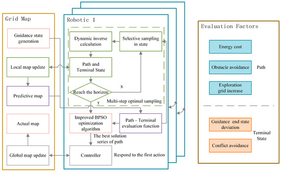
Figure 1.
Distributed Next-Best-Path and Terminal exploration framework.
The left side of Figure 1 shows the DNBPT framework we propose. We set a prediction horizon as the time domain for each plan and plan the series paths of the UAV with a fixed length. We take a multistep sampling and preferential growth method, sample in a limited state space, and inversely calculate the dynamic path through the terminal state to obtain the path and terminal state. Considering the factors mentioned above to evaluate, we select a certain number of action sequences with high evaluation. Due to the nonoptimal solution by limited sampling, the series of paths obtained is used as the initial solution of the improved BPSO algorithm to further optimize and finally obtain the optimal path and terminal sequence. The controller responds to the first step of the optimal sequence to address sudden obstacles or other situations in the actual movement. In this framework, UAVs can join or leave the exploration mission freely without causing disorder in the whole system.
2.2. Exploration Model in Unknown Environments
The dynamics of the UAV have the property of differential flatness [32]. In the planning process, the flat output is used as the planning quantity to reduce the planning dimension and improve the timeliness. is the position of the UAV and is the yaw angle.
The obtained detection area is fitted with the local grid map to obtain the index of the grid map and bring it into the global map, as shown in Equation (1).
Assume that k is the length of the prediction horizon and is the state sequence in the prediction horizon as the input of the predictive map update and the evaluation function.
The UAV carries sensors with an observation field of view (FOV) to detect environmental information. In this paper, the sensor mapping algorithm is not considered, and it is assumed that the sensor can obtain the environment information within the angle range. The sensor can be equivalent to a sector, and its detection range within the prediction interval can identify the trajectory of the sensor’s sector area driven by the k segment control for integration, as shown in Equation (2), where represents the processing program of the region on the grid map and represents the number of new grids.
Due to the complexity of the integral calculation and the grid form of the map, we propose a simplification to predict the update of the map and calculate the number of new detection grids, as shown in Figure 2. The sampling range and time interval are limited to ensure that the state falls in the previous detection sector. For a state in the terminal state sequence , we connect the two points and of the previous sector and the two points and of the current sector. A convex quadrilateral is formed, and each convex quadrilateral is connected. The obtained convex quadrilateral is placed into the local map to calculate the number of new exploration grids as the evaluation basis of the path-terminal sequence, as shown in Equation (3).
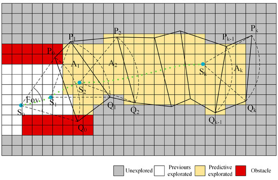
Figure 2.
Detection model and approximate calculation of grid increase.
This equivalent method improves the calculation efficiency to support online UAV planning.
2.3. Construction of the Evaluation Function
In the process of exploring the unknown environment, the form of the solution is the terminal state sequence of the predicted horizon and the path between the state transitions. Its optimality evaluation includes two aspects: the path and the terminal state.
First, the path needs to be checked for obstacle conflicts, and it is necessary to ensure that the planned path of the cluster will not collide with the obstacles that have been explored. The path points in the process are extracted by interpolation, and the obstacle is checked in the grid map. The results are accumulated for the evaluation function value, such as Equation (4). Note that this is not applied in sampling but in the optimization algorithm.
In the action space, under the constraint conditions, the average energy consumption of the action sequence is smallest, as shown in Equation (5), where dim (u) is the dimension of the action space.
To ensure the continuity and smoothness of the front and back actions, it is necessary to minimize the front and back deviation of each step in the action sequence, as shown in Equation (6):
The exploration of unknown space during the UAV’s movement brings gain. The calculation method of the number of new exploration grids is proposed above, and the evaluation function is shown in Equation (7). refers to the number of exploration grids in the ideal state. The calculation method is shown in Equation (8), where is the sensor detection distance, is the fixed maximum distance for sampling, and is the map resolution (magnification).
Because the environment is unknown, the exploration gain under different paths may be similar. In the later stage of the exploration process, it may occur that the UAV’s surrounding environment has been completely explored. It is easy to fall into the local optimum, causing invalid and repeated paths. Therefore, the guidance of other factors is needed to enable the UAV to move in the direction that the gain may increase. The rating function of this part is shown as Equation (9):
where is the state at moment , is the initial state, and is the reference guidance state. We use frontier coordinates and straight orientation as references in this paper, and the frontier is rapidly generated through the edge detection of OpenCV.
To improve the exploration efficiency of the cluster, the UAVs should be distributed as far as possible. Therefore, the evaluation function is designed for the terminal state, as in Equation (10), where is the set safety distance and is the number of UAVs in the cluster.
Based on the above evaluation factors, the total evaluation functions used in selective sampling and improved BPSO, respectively, are designed as Equations (11) and (12), respectively:
where is the weight value, which can be adjusted according to the actual situation, while .
3. Method and Algorithm
3.1. Multistep Selective Sampling Algorithm
To make UAVs better adapt to unknown environments, planning is often performed in multiple steps. Planning the multipath within a certain planning horizon and executing the first segment of the optimal path are needed. In the calculation process, the number of samples will increase exponentially with the increase in the number of segments in the planning horizon, and the calculation cost is unaffordable. Therefore, we design a multistep selective sampling method. During each round of sampling, we sample the sequence with high current evaluation in the next step. The pseudocode of Algorithm 1 shows more details of the multistep selective sampling method.
An empty set saves path and terminal sequences with lengths less than , and an empty set saves sequences with lengths equal to . In the sampling space under the constraint conditions, terminal states are randomly taken to be composed on the initial state as the initial sequence, and then the loop begins while the sequence gradually grows. In each loop, the best solutions in the set are selected for the next step of sampling. Each solution also takes states randomly in the updated sampling space based on the current state to make the sequence grow and update these sequences in . The sequence with a length of is placed in and will not be selected again for the next sampling. When the evaluation value of the th better sequence in is greater than the best evaluation value of the sequence in , the sampling process is finished.
After multistep selective sampling, path and terminal state sequences are obtained as the basis of the next optimization algorithm.
| Algorithm 1 Multistep selective sampling |
| Input: Grid Map, initial state , sample space , other states Parameters: planning horizon , number of samples , , safe distance Output: aggregate of terminal state sequence with path |
| update sampling random m in , generate , while is not empty select the best sequences with length < update uniform sampling in based on the selected sequences , update the evalution value of //according to the Equation (11) if then else if the th best in better than the best in then break select the best n in as output |
3.2. Improved Discrete Binary Particle Swarm Optimization Algorithm
To select the optimal path from the generated multiple paths, we propose an optimal path selection method based on improved BPSO. We propose a mutation strategy to increase the diversity of the population, which can help the particle swarm jump out of the local optimum trap. In addition, we introduce a contraction factor to ensure the convergence performance of the algorithm [33], which controls the final convergence of the system behavior and can effectively search different regions. This method can obtain high-quality solutions.
The velocity and position update formulas of the particle swarm after introducing the contraction factor is shown as Equations (13) and (14), respectively:
where represents the shrinkage factor, as shown in Equation (15), represents the current iteration number, and are the learning factors [34,35,36], and are two random values uniformly distributed in [0, 1], and and represent the individual optimal position and the global optimal position of the particle, respectively.
Our mutation strategy introduces the idea of the dMOPSO [37] algorithm, and age is used to represent the number of times that the individual optimal position () of the current particle has not been updated continuously in the loop. When the local optimal position of the particle has not been updated for a long time, it means that the particle is likely to have fallen into the local optimal position, and it is necessary to perturb the particle. The specific perturbation example is shown in Figure 3.
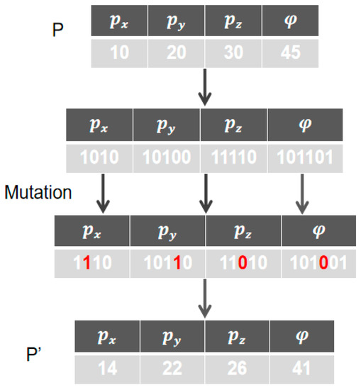
Figure 3.
Perturbing the particles that have been in the local optimum for a long time.
The state of particles is converted into binary form. In each coordinate, a bit of the position is randomly selected for the mutation operation. After the mutation operation, the particle’s age is reset to 0. If the particle’s age does not reach the age threshold, only the particle’s age is increased. The pseudocode of the mutation operation is shown in Algorithm 2:
| Algorithm 2 Mutation strategy |
| Input: Pop(swarm), , (size of the population), (threshold of age) Output: NewPop(new swarm) |
| for = 1 : do if > Ta then Mutation() Fitness ← CalculateFitness() //according to the Equation (12) if fitness() > fitness() then 0 else + 1 end if end for return NewPop |
The proposed improved BPSO algorithm is mainly divided into two stages. The first stage is the initialization stage. We encode and initialize the particle swarm according to the input path information, randomly initialize the speed and the age of the initialization particle, and finally calculate the fitness value of the particle. The second stage is the main loop stage. When the particle’s age exceeds the age threshold, the mutation operation is performed. The loop is finished when the termination condition is met. The final returned is the optimal sequence of terminals with paths. The pseudocode of the Algorithm 3 is:
| Algorithm 3 Improved DBPSO |
| Input: original Pop, size of the population , maximal generation number maxgen Output: (optimal sequence of terminal state with path) |
| P ← InitializeParticles() Age ← InitializeAge() Fitness ← CalculateFitness() While NCT (Number of current iterations) <= maxgen do for = 1 : do ←SelectGbest(Pop) Pop ← Updateparticles(N) //according to the Equations (13)–(15) Mutation() Fitness ← CalculateFitness(N) //according to the Equation (12) Pop ← NewPop ← SelectGbest(Pop) end for end while return |
4. Simulation and Analysis
4.1. Simulation in Fixed-Obstacle Scenes
We design three indoor scenes with fixed obstacles of different sizes based on the interior of the building, and the number of UAVs in each scene is different. Due to the indoor scene, we assume that the UAV is flying at a fixed altitude. The sizes of the scene are 20 m long and 50 m wide, 50 m long and 50 m wide, and 100 m long and 100 m wide, respectively. The numbers of UAVs are 3, 4, and 5. For each scene, simulations of a fixed initial state and a random initial state are carried out. The initial states of all scenes are shown in Figure 4a, Figure 5a, Figure 6a, Figure 7a, Figure 8a and Figure 9a. More detailed parameters about the scenes and algorithm are shown in Table 1 and Table 2.
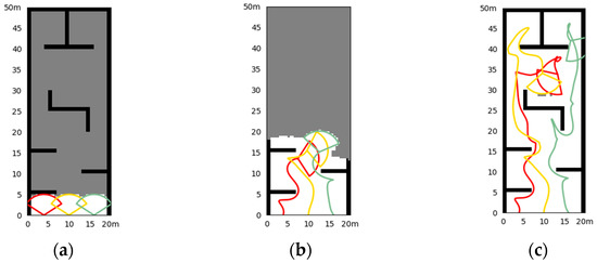
Figure 4.
Simulation results of the fixed initial state in Scene I. (a) The initial state of the simulation and the obstacle; (b) the situation at a certain moment (10.8 s) in the exploration process; (c) the situation of exploration results.
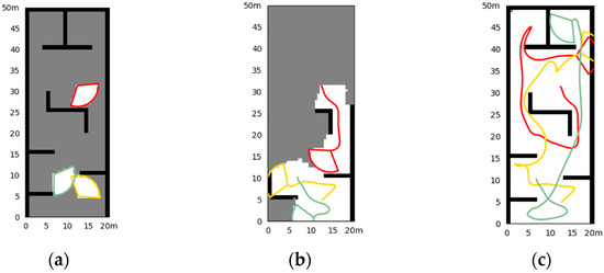
Figure 5.
Simulation results of the random initial state in Scene I. (a) The initial state of the simulation and the obstacle; (b) the situation at a certain moment (8.4 s) in the exploration process; (c) the situation of exploration results.
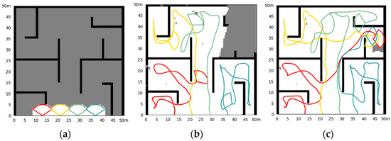
Figure 6.
Simulation results of the fixed initial state in Scene II. (a) The initial state of the simulation and the obstacle; (b) the situation at a certain moment (46.8 s) in the exploration process; (c) the situation of exploration results.
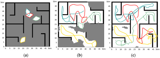
Figure 7.
Simulation results of the random initial state in Scene II. (a) The initial state of the simulation and the obstacle; (b) the situation at a certain moment (34.0 s) in the exploration process; (c) the situation of exploration results.
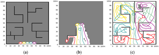
Figure 8.
Simulation results of the fixed initial state in Scene III. (a) The initial state of the simulation and the obstacle; (b) the situation at a certain moment (20.0 s) in the exploration process; (c) the situation of exploration results.
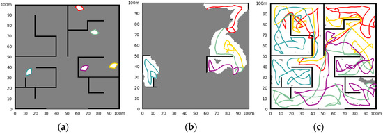
Figure 9.
Simulation results of the random initial state in Scene III. (a) The initial state of the simulation and the obstacle; (b) the situation at a certain moment (25.6 s) in the exploration process; (c) the situation of exploration results.

Table 1.
Parameter setting for three scenes.
Table 2.
Parameter setting for three algorithms.
- Simulation in Scene I
Figure 4 shows the simulation results of three UAV explorations in Scene I, with fixed initial UAV states to start. The exploration takes 36.8 s. It can be seen that the cluster can realize well the exploration of the environment in a short time, and there are few repeated paths, unless it is necessary to leave the impasse that is surrounded by obstacles. Figure 5 shows the results of random initial states, and the exploration takes 34.6 s. We can see that the cluster can explore well in any initial state, with the same short time cost and fewer repeated paths.
- 2.
- Simulation in Scene II
Figure 6 shows the simulation results of four UAV explorations in Scene II, with fixed initial UAV states to start. The exploration takes 62.0 s. Figure 7 shows the results of random initial states, and the exploration takes 63.2 s. In medium-size scenes, UAVs in the cluster avoid repeated exploration in the same area through a distributed strategy. The UAV can quickly return to exploring other areas after the exploration of corners or the impasse. In the random initial state, the UAV’s performance is almost unaffected.
- 3.
- Simulation in Scene III
Figure 8 shows the simulation results of four UAV explorations in Scene III, with fixed initial UAV states to start, and Figure 9 shows the situation of random initial states. Exploration takes 190.0 s and 214.8 s, respectively.
With the expansion of the scale of the exploration scene and the increase in the complexity of the internal structure, the difficulty of cluster exploration is also increasing, and the UAVs show a complex movement. The random initial state brings uncertainty to the exploration process. Under the above factors, whether the exploration efficiency can be maintained is the key point of the exploration method. The proposed method can still maintain the complete exploration of the area in large scenes, and there is less repeated exploration. There may be a tendency for multiple UAVs to move in the same direction at the end of the exploration. This is because we do not allow the UAV to be idle, to achieve the fastest exploration speed. As the environment is unknown, it is difficult to define which UAV can reach the unexplored area faster, so we keep every UAV in the cluster continuously exploring until the area is fully explored. This ensures the shortest exploration time, but may bring a waste of energy for engineering applications. It can be adjusted according to the actual application, for example, using conditional judgments to make some UAVs idle.
- 4.
- Comparing the methods in three scenes
Due to the randomness of the environment exploration process, we conduct 100 simulations for each situation (fixed initial state and random initial state in each scene) and count the time cost of exploration and compare it with the two classical methods, as shown in Table 3. The frontier-based method is a method with fixed results when the frontier generation, map, and initial state are fixed. The NBV and DNBPT methods have some randomness in the process for deeper exploration. The average exploration efficiency of a single UAV in all scenes is also compared, as shown in Figure 10.
Table 3.
Results and comparison of multiple simulation data samples in the fixed obstacle scenes.
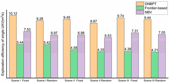
Figure 10.
Comparison of the single UAV exploration efficiency of each method.
Compared with the frontier-based method and the NBV, the exploration efficiency of the proposed method in each scene has a great advance. In Scene I, the exploration efficiency is increased on average by approximately 85.7% and 34.4% with fixed initial states and 71.4% and 33.1% with random initial states, respectively. In Scene II, the efficiency is increased by approximately 107.0% and 36.0% with fixed initial states and 108.7% and 35.8% with random initial states, respectively. In Scene III, the efficiency is increased by approximately 122.1% and 36.6% with fixed initial states and by 124.4% and 33.9% with random initial states, respectively. For larger and more complex indoor scenes, the improvement effect of the proposed method is more obvious.
In the simulation process of algorithm comparison, it is found that the frontier-based method has a good effect in the early stage of exploration. However, in the end stage, due to its greedy strategy that tends to the nearest point, many omissions in the early stage need to be explored in reverse, resulting in a waste of efficiency. This becomes more obvious with increasing exploration rate requirements. The NBV method can carry out deeper exploration locally, but it loses the directional guidance of the global environment and produces repeated meaningless paths. The proposed method combines the advantages of the two methods, including deep local exploration and global guidance, to improve the exploration efficiency of UAV clusters and reduce repetitive paths.
This proves the effectiveness and superiority of the method in complex indoor scenes. In addition, the proposed method shows a stabler exploration efficiency in uncertain scenes and can complete the exploration quickly in any initial state.
4.2. Simulation in Random-Obstacle Scenes
To explore the applicability of our method in other scenes, we design a random obstacle scene for simulation. We simulate scenes with dense small obstacles such as trees, where obstacles are randomly generated and their size is limited, as shown in Figure 11. We also design the situations of a fixed initial state and a random initial state. The scene size is set to be 100 m long and 30 m wide, and four UAVs form a cluster. The number of obstacles in the scene is 40, and the maximum side length of obstacles is 3 m. The simulation is also designed for constant-altitude flight. The initial state of the UAV in fixed scenes is (0, 3, 0), (0, 11, 0), (0, 19, 0), and (0, 27, 0). The terminal condition for exploration is that the map exploration rate reaches 99%.
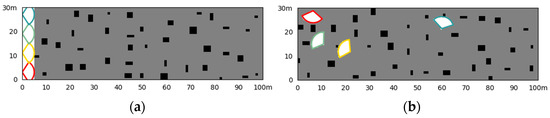
Figure 11.
Scene with randomly dense small obstacles. (a) The situation of the fixed initial UAV states; (b) the situation of random initial UAV states.
Similarly, we conduct 100 simulations for a fixed initial state and a random initial state and compare them with other algorithms. The simulation results of once in each scene are shown in Figure 12 and Figure 13, and the statistical data are shown in Table 4. Under the condition of fixed initial states, the cluster can complete the exploration with few repeated backtrackings and a high rate of coverage while crossing the obstacle area. The random initial state has an impact on the exploration, leading to more possible backtrack and repetitions, but it can still be handled well for reduction.
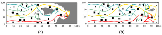
Figure 12.
Simulation results of the fixed initial state. (a) The situation at a certain moment (41.2 s) in the exploration process; (b) the situation of exploration results (64.0 s).
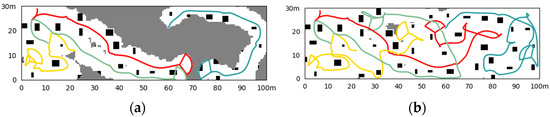
Figure 13.
Simulation results of the random initial state. (a) The situation at a certain moment (36.0 s) in the exploration process; (b) the situation of exploration results (72.4 s).
Table 4.
Results and comparison of multiple simulation data samples in random obstacle scene.
Regarding the exploration of areas with dense small obstacles, compared with the frontier-based method and NBV, the exploration efficiency is increased on average by approximately 37.4% and 25.2% with fixed initial states and 40.1% and 24.8% with random initial states, respectively. The comparison proves the good performance in the environment with dense small obstacles.
5. Conclusions
In this paper, we propose a DNBPT method for UAV clusters to explore unknown environments. The gain is calculated by comprehensively considering the contribution of the path process and the terminal state to the exploration, and the optimal path is evaluated and selected by multistep optimal sampling and the improved BPSO algorithm. The simulation results show that this method has advantages in different types and sizes of scenes. In addition, this method has strong generality and can be transplanted to other robot platforms.
Author Contributions
Conceptualization, Y.W. and X.L.; methodology, Y.W. and X.L.; software, X.L.; validation, X.L. and X.Z.; formal analysis, X.L., X.Z., F.L. and Y.L.; investigation, F.L. and Y.L.; resources, Y.W.; writing—original draft preparation, X.L.; writing—review and editing, Y.W. and X.Z.; supervision, Y.W. All authors have read and agreed to the published version of the manuscript.
Funding
This research received no external funding.
Data Availability Statement
Not applicable.
Conflicts of Interest
The authors declare no conflict of interest.
References
- Zheng, Y.-J.; Du, Y.-C.; Ling, H.-F.; Sheng, W.-G.; Chen, S.-Y. Evolutionary Collaborative Human-UAV Search for Escaped Criminals. IEEE Trans. Evol. Comput. 2019, 24, 217–231. [Google Scholar] [CrossRef]
- Unal, G. Visual Target Detection and Tracking Based on Kalman Filter. J. Aeronaut. Space Technol. 2021, 14, 251–259. [Google Scholar]
- Alotaibi, E.T.; Alqefari, S.S.; Koubaa, A. Lsar: Multi-uav Collaboration for Search and Rescue Missions. IEEE Access 2019, 7, 55817–55832. [Google Scholar] [CrossRef]
- Yang, Y.; Xiong, X.; Yan, Y. UAV Formation Trajectory Planning Algorithms: A Review. Drones 2023, 7, 62. [Google Scholar] [CrossRef]
- Chen, Y.; Dong, Q.; Shang, X.; Wu, Z.; Wang, J. Multi-UAV Autonomous Path Planning in Reconnaissance Missions Considering Incomplete Information: A Reinforcement Learning Method. Drones 2022, 7, 10. [Google Scholar] [CrossRef]
- Chi, W.; Ding, Z.; Wang, J.; Chen, G.; Sun, L. A Generalized Voronoi Diagram-based Efficient Heuristic Path Planning Method for RRTs in Mobile Robots. IEEE Trans. Ind. Electron. 2021, 69, 4926–4937. [Google Scholar] [CrossRef]
- Sun, Y.; Tan, Q.; Yan, C.; Chang, Y.; Xiang, X.; Zhou, H. Multi-UAV Coverage through Two-Step Auction in Dynamic Environments. Drones 2022, 6, 153. [Google Scholar] [CrossRef]
- Cheng, L.; Yuan, Y. Adaptive Multi-player Pursuit–evasion Games with Unknown General Quadratic Objectives. ISA Trans. 2022, 131, 73–82. [Google Scholar] [CrossRef]
- Elsisi, M. Improved Grey wolf Optimizer Based on Opposition and Quasi Learning Approaches for Optimization: Case Study Autonomous Cehicle Including Vision System. Artif. Intell. Rev. 2022, 55, 5597–5620. [Google Scholar] [CrossRef]
- Batinovic, A.; Petrovic, T.; Ivanovic, A.; Petric, F.; Bogdan, S. A Multi-resolution Frontier-based Planner for Autonomous 3D Exploration. IEEE Robot. Autom. Lett. 2021, 6, 4528–4535. [Google Scholar] [CrossRef]
- Gomez, C.; Hernandez, A.C.; Barber, R. Topological Frontier-based Exploration and Map-building Using Semantic Information. Sensors 2019, 19, 4595. [Google Scholar] [CrossRef] [PubMed]
- Tang, C.; Sun, R.; Yu, S.; Chen, L.; Zheng, J. Autonomous Indoor Mobile Robot Exploration Based on Wavefront Algorithm. In Intelligent Robotics and Applications: 12th International Conference, ICIRA 2019, Shenyang, China, 8–11 August 2019; Proceedings, Part V 12, 2019; Springer: Berlin/Heidelberg, Germany, 2019; pp. 338–348. [Google Scholar]
- Ahmad, S.; Mills, A.B.; Rush, E.R.; Frew, E.W.; Humbert, J.S. 3d Reactive Control and Frontier-based Exploration for Unstructured Environments. In Proceedings of the 2021 IEEE/RSJ International Conference on Intelligent Robots and Systems (IROS), Prague, Czech Republic, 27 September–1 October 2021; IEEE: Piscataway, NJ, USA, 2021; pp. 2289–2296. [Google Scholar]
- Cieslewski, T.; Kaufmann, E.; Scaramuzza, D. Rapid Exploration with Multi-rotors: A Frontier Selection Method for High Speed Flight. In Proceedings of the 2017 IEEE/RSJ International Conference on Intelligent Robots and Systems (IROS), Vancouver, BC, Canada, 24–28 September 2017; IEEE: Piscataway, NJ, USA, 2017; pp. 2135–2142. [Google Scholar]
- Zhou, B.; Zhang, Y.; Chen, X.; Shen, S. Fuel: Fast Uav Exploration Using Incremental Frontier Structure and Hierarchical Planning. IEEE Robot. Autom. Lett. 2021, 6, 779–786. [Google Scholar] [CrossRef]
- Ashutosh, K.; Kumar, S.; Chaudhuri, S. 3d-nvs: A 3D Supervision Approach for Next View Selection. In Proceedings of the 2022 26th International Conference on Pattern Recognition (ICPR), Montreal, QC, Canada, 21–25 August 2022; IEEE: Piscataway, NJ, USA, 2022; pp. 3929–3936. [Google Scholar]
- Kim, J.; Bonadies, S.; Lee, A.; Gadsden, S.A. A Cooperative Exploration Strategy with Efficient Backtracking for Mobile Robots. In Proceedings of the 2017 IEEE International Symposium on Robotics and Intelligent Sensors (IRIS), Ottawa, ON, Canada, 5–7 October 2017; IEEE: Piscataway, NJ, USA, 2017; pp. 104–110. [Google Scholar]
- Palazzolo, E.; Stachniss, C. Effective Exploration for MAVs Based on the Expected Information Gain. Drones 2018, 2, 9. [Google Scholar] [CrossRef]
- Li, J.; Li, C.; Chen, T.; Zhang, Y. Improved RRT Algorithm for AUV Target Search in Unknown 3D Environment. J. Mar. Sci. Eng. 2022, 10, 826. [Google Scholar] [CrossRef]
- Vasquez-Gomez, J.I.; Troncoso, D.; Becerra, I.; Sucar, E.; Murrieta-Cid, R. Next-best-view Regression Using a 3D Convolutional Neural Network. Mach. Vis. Appl. 2021, 32, 1–14. [Google Scholar]
- Duberg, D.; Jensfelt, P. Ufoexplorer: Fast and Scalable Sampling-based Exploration with a Graph-based Planning Structure. IEEE Robot. Autom. Lett. 2022, 7, 2487–2494. [Google Scholar] [CrossRef]
- Wang, J.; Li, T.; Li, B.; Meng, M.Q.-H. GMR-RRT*: Sampling-based path Planning Using Gaussian Mixture Regression. IEEE Trans. Intell. Veh. 2022, 7, 690–700. [Google Scholar] [CrossRef]
- Li, H.; Zhang, Q.; Zhao, D. Deep Reinforcement Learning-based Automatic Exploration for Navigation in Unknown Environment. IEEE Trans. Neural Netw. Learn. Syst. 2019, 31, 2064–2076. [Google Scholar] [CrossRef]
- Ramezani Dooraki, A.; Lee, D.-J. An End-to-end Deep Reinforcement Learning-based Intelligent Agent Capable of Autonomous Exploration in Unknown Environments. Sensors 2018, 18, 3575. [Google Scholar] [CrossRef]
- Niroui, F.; Zhang, K.; Kashino, Z.; Nejat, G. Deep Reinforcement Learning Robot for Search and Rescue Applications: Exploration in Unknown Cluttered Environments. IEEE Robot. Autom. Lett. 2019, 4, 610–617. [Google Scholar] [CrossRef]
- Garaffa, L.C.; Basso, M.; Konzen, A.A.; de Freitas, E.P. Reinforcement Learning For Mobile Robotics Exploration: A Survey. IEEE Trans. Neural Netw. Learn. Syst. 2021, 1–15. [Google Scholar] [CrossRef]
- Xu, Y.; Yu, J.; Tang, J.; Qiu, J.; Wang, J.; Shen, Y.; Wang, Y.; Yang, H. In Explore-bench: Data Sets, Metrics and Evaluations for Frontier-based and Deep-reinforcement-learning-based Autonomous Exploration. In Proceedings of the 2022 International Conference on Robotics and Automation (ICRA), Philadelphia, PA, USA, 23–27 May 2022; IEEE: Piscataway, NJ, USA, 2022; pp. 6225–6231. [Google Scholar]
- Elmokadem, T.; Savkin, A.V. Computationally-Efficient Distributed Algorithms of Navigation of Teams of Autonomous UAVs for 3D Coverage and Flocking. Drones 2021, 5, 124. [Google Scholar] [CrossRef]
- Unal, G. Fuzzy Robust Fault Estimation Scheme for Fault Tolerant Flight Control Systems Based on Unknown Input Observer. Aircr. Eng. Aerosp. Technol. 2021, 93, 1624–1631. [Google Scholar] [CrossRef]
- Kilic, U.; Unal, G. Aircraft Air Data System Fault Detection and Reconstruction Scheme Design. Aircr. Eng. Aerosp. Technol. 2021, 93, 1104–1114. [Google Scholar] [CrossRef]
- Hong, Y.; Kim, S.; Kim, Y.; Cha, J. Quadrotor Path Planning Using A* Search Algorithm and Minimum Snap Trajectory Generation. ETRI J. 2021, 43, 1013–1023. [Google Scholar] [CrossRef]
- Unal, G. Integrated Design of Fault-tolerant Control for Flight Control Systems Using Observer and Fuzzy logic. Aircr. Eng. Aerosp. Technol. 2021, 93, 723–732. [Google Scholar] [CrossRef]
- Amoozegar, M.; Minaei-Bidgoli, B. Optimizing Multi-objective PSO Based Feature Selection Method Using a Feature Elitism Mechanism. Expert Syst. Appl. 2018, 113, 499–514. [Google Scholar] [CrossRef]
- Yuan, Q.; Sun, R.; Du, X. Path Planning of Mobile Robots Based on an Improved Particle Swarm Optimization Algorithm. Processes 2022, 11, 26. [Google Scholar] [CrossRef]
- Han, F.; Chen, W.-T.; Ling, Q.-H.; Han, H. Multi-objective Particle Swarm Optimization with Adaptive Strategies for Feature Selection. Swarm Evol. Comput. 2021, 62, 100847. [Google Scholar] [CrossRef]
- Han, F.; Wang, T.; Ling, Q. An Improved Feature Selection Method Based on Angle-guided Multi-objective PSO and Feature-label Mutual Information. Appl. Intell. 2023, 53, 3545–3562. [Google Scholar] [CrossRef]
- Shaikh, P.W.; El-Abd, M.; Khanafer, M.; Gao, K. A Review on Swarm Intelligence and Evolutionary Algorithms for Solving the Traffic Signal Control Problem. IEEE Trans. Intell. Transp. Syst. 2020, 23, 48–63. [Google Scholar] [CrossRef]
Disclaimer/Publisher’s Note: The statements, opinions and data contained in all publications are solely those of the individual author(s) and contributor(s) and not of MDPI and/or the editor(s). MDPI and/or the editor(s) disclaim responsibility for any injury to people or property resulting from any ideas, methods, instructions or products referred to in the content. |
© 2023 by the authors. Licensee MDPI, Basel, Switzerland. This article is an open access article distributed under the terms and conditions of the Creative Commons Attribution (CC BY) license (https://creativecommons.org/licenses/by/4.0/).