Comparative Assessment of Vegetation Removal for DTM Generation and Earthwork Volume Estimation Using RTK-UAV Photogrammetry and LiDAR Mapping

Highlights

What are the main findings?

• Combining a color-based vegetation index with a geometry-based filter greatly enhanced DTM accuracy; the ExGR + Lasground (new) combination achieved RMSE 0.179 m for UAV photogrammetry and 0.165 m for LiDAR.
• Both UAV-based methods showed reliable earthwork volume accuracy, reaching 100.9% for photogrammetry and 100.3% for LiDAR even in densely vegetated terrain.

What are the implications of the main findings?

• The integrated LiDAR + ExGR + Lasground (new) method is recommended for high-precision terrain modeling and construction surveying.
• UAV photogrammetry offers a cost-effective and efficient alternative when LiDAR use is limited by budget or operational conditions.

Abstract

Earthwork volume calculation is a fundamental process in civil engineering and construction, requiring high-precision terrain data to assess ground stability encompassing load-bearing capacity, susceptibility to settlement, and slope stability and to ensure accurate cost estimation. However, seasonal and environmental constraints pose significant challenges to surveying. This study employed unmanned aerial vehicle (UAV) photogrammetry and light detection and ranging (LiDAR) mapping to evaluate the accuracy of digital terrain model (DTM) generation and earthwork volume estimation in densely vegetated areas. For ground extraction, color-based indices (excess green minus red (ExGR), visible atmospherically resistant index (VARI), green-red vegetation index (GRVI)), a geometry-based algorithm (Lasground (new)) and their combinations were compared and analyzed. The results indicated that combining a color index with Lasground (new) outperformed the use of single techniques in both photogrammetric and LiDAR-based surveying. Specifically, the ExGR–Lasground (new) combination produced the most accurate DTM and achieved the highest precision in earthwork volume estimation. The LiDAR-based results exhibited an error of only 0.3% compared with the reference value, while the photogrammetric results also showed only a slight deviation, suggesting their potential as a practical alternative even under dense summer vegetation. Therefore, although prioritizing LiDAR in practice is advisable, this study demonstrates that UAV photogrammetry can serve as an efficient supplementary tool when cost or operational constraints are present.

1. Introduction

Earthwork volume calculation is a crucial procedure in the initial design stage of civil engineering projects, serving as fundamental data for preliminary cost estimation and ensuring ground stability. It must be conducted early to assess the overall constructability of the project, making the acquisition of accurate ground data essential. Traditionally, manual-based methods such as the contour method, spot elevation method, and average end area method have been primarily used; however, they present limitations in terms of work efficiency and precision [1]. With advances in total station and global navigation satellite system (GNSS) technology, the virtual reference station (VRS) method has been widely adopted. Owing to its high coordinate accuracy, it has also been utilized as a benchmark in academic research related to various earthwork projects [2,3]. Nevertheless, VRS surveying has inherent constraints: it is highly demanding in terms of manpower and time for large or undulating terrains, and achieving precise measurements in steep, densely vegetated, or rocky areas remains challenging due to limited accessibility. Consequently, the need for alternative technologies capable of reliably acquiring ground data irrespective of seasonal or terrain conditions has emerged. In response, remote sensing techniques including image-based aerial photogrammetry and reflected light-based LiDAR sensing have gained increasing attention as potential alternatives [4].

Recently, the introduction of unmanned aerial vehicle (UAV)-based remote sensing has further expanded the scope of application to various fields, including earthwork volume estimation [5]. UAV surveying has been applied to diverse domains such as land cover classification in agricultural regions and mining terrain analysis due to its lower operational costs and greater portability compared with conventional aerial surveys [6,7,8,9]. Moreover, UAVs provide flexibility in altitude control and can be equipped with a range of payloads, enabling the efficient acquisition of high-density data within a short period, even in areas with limited human accessibility. Leveraging these advantages, Hugenholtz et al. (2015) verified the accuracy of UAV photogrammetry for earthwork volume estimation in a bare-earth environment [10], and Seong et al. (2018) conducted a comparative study of VRS, photogrammetry, and total station surveying in a levee area [11]. Park et al. (2021) compared post-processing results of photogrammetry and LiDAR in sloped terrain, demonstrating the superiority of LiDAR [12], whereas Kang et al. (2024) showed that both photogrammetry and LiDAR achieved consistent accuracies exceeding 95%, regardless of the presence of ground control points (GCPs) [13]. In another case, unsupervised classification based on LiDAR intensity was used to separate cut and fill components, followed by an economic analysis that considered the need for additional soil supply [14]. However, most previous studies have focused on a single imaging technique or coordinate dataset, and few have integrated both the optical information from photogrammetry and LiDAR into earthwork volume estimation. Although several studies have evaluated ground surface reconstruction using photogrammetry [4], systematic comparisons incorporating LiDAR remain scarce. Furthermore, empirical research quantitatively analyzing the influence of reconstruction performance differences on actual earthwork volume estimation is extremely limited. Hence, comparative studies are needed to investigate how the differences between photogrammetry and LiDAR affect the accuracy of earthwork volume estimation.

In this context, the application of filtering techniques tailored to the unique characteristics of photogrammetric and LiDAR data has emerged as a critical strategy to improve ground surface reconstruction accuracy and its linkage to earthwork volume estimation [15,16]. For example, Anders et al. (2019) successfully extracted ground points from vegetation-covered UAV photogrammetric data by applying multiple filtering techniques [17]. Kraus and Pfeifer (1998) also developed an iterative surface-weighting interpolation method that enabled ground extraction even in dense forested areas, laying the foundation for photogrammetry and LiDAR-based filtering research using point clouds [18]. Building upon this, Kim and Cho (2012) proposed a grid-based filtering technique that classifies points within a specified elevation tolerance as ground [19]. Other studies have reported effective ground separation through optical indices derived from RGB data captured by LiDAR [20]. The vegetation-removal performance of LiDAR can be further enhanced by utilizing intensity values acquired at laser wavelengths that vary depending on the sensor. In this context, LiDAR intensity represents the laser backscatter characteristics from objects and is fundamentally different, in terms of physical measurement principles and interpretation, from near-infrared (NIR) reflectance values obtained from optical multispectral sensors used for vegetation indices. In this regard, the laser wavelength employed varies among LiDAR sensors, and the LiDAR sensor used in this study operated at a laser wavelength of approximately 905 nm. Accordingly, the effectiveness of intensity-based vegetation discrimination depends on the characteristics of the LiDAR sensor itself rather than on optical NIR imagery. Wei et al. (2017) achieved a lower root mean square error (RMSE) than commercial software using a RANSAC-based plane estimation filter that employed LiDAR intensity [21]. A subsequent comparative study identified intensity as one of seven major factors affecting filtering quality, emphasizing its importance for object separation in complex terrains [22]. Conversely, photogrammetry remains a cost-effective and easy-to-operate alternative; some studies have even shown that high-resolution RGB information allows photogrammetry to surpass LiDAR accuracy under certain conditions [23]. Deep learning applications have further improved UAV photogrammetry-based ground extraction in complex environments [24], and comparative studies with terrestrial laser scanning (TLS) have recommended UAV photogrammetry as a more efficient solution in lowland regions with dense vegetation [25]. Overall, both methods exhibit complementary strengths and weaknesses. Therefore, rather than a single-platform approach, a comprehensive comparative analysis considering the respective characteristics, advantages, and limitations of each platform is necessary. Quantitative evaluation of ground surface reconstruction and earthwork volume estimation performance under identical conditions will enable the selection of an optimal surveying method that ensures both precision and practicality.

Therefore, this study applies vegetation filtering techniques that integrate terrain characteristics—such as RGB spectral information and three-dimensional spatial coordinates—to extract ground points from UAV photogrammetry and LiDAR data acquired sequentially at the same site and on the same day. Through this process, we quantitatively compare ground surface reconstruction performance and earthwork volume estimation accuracy in areas with dense, low-lying vegetation. In particular, by analyzing the performance differences in identical vegetation filtering methods applied to both photogrammetric and LiDAR data, this study seeks to fill the gap in direct performance comparisons between these platforms. Ultimately, the objectives of this research are twofold: (1) to analyze the influence of digital terrain model (DTM) generation performance from each platform on the accuracy of earthwork volume estimation, and (2) to propose an efficient and practical alternative that minimizes seasonal constraints and reduces on-site labor requirements.

2. Materials and Methods

2.1. Methodology

In this study, based on the results of a traditional VRS survey as the reference, photogrammetry and LiDAR surveys were conducted using a rotary-wing UAV over a levee slope during the summer season, when vegetation was most vigorous, to construct a fully georeferenced 3D model with corrected baseline coordinates. Subsequently, seven common vegetation removal methods were applied to the datasets acquired from each surveying technique. Considering the characteristics of each dataset, ground extraction was performed using methods that utilized (1) red-green-blue spectral information alone, (2) geometric characteristics, and (3) a sequential combination of both. After filtering, the areas where vegetation had been removed were reconstructed into a DTM using a statistical interpolation method. The performance of this ground surface reconstruction was then quantitatively evaluated by comparing the generated DTM with the reference DTM derived from the VRS survey and by calculating accuracy assessment metrics such as root mean square error and mean absolute error (MAE). Finally, each digital terrain model was converted into a triangular irregular network (TIN) model, which was used to calculate the earthwork volume. Through this entire process, the accuracy of each platform and its practical applicability to construction sites were comprehensively compared and analyzed (Figure 1).

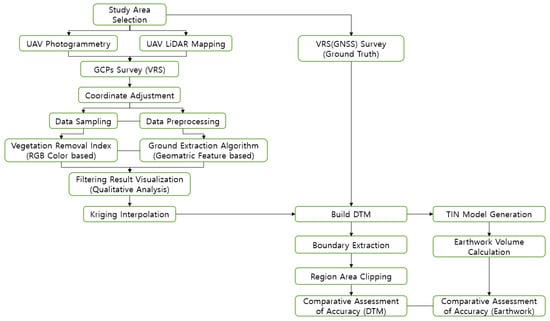
Figure 1. Research Flow Chart.

2.2. Study Area and Survey Equipment

2.2.1. Study Area

The study was conducted in the area of an agricultural reservoir located at 312 Sangyong-ri, Hwaseo-myeon, Sangju-si, Gyeongsangbuk-do, Republic of Korea (latitude: 36.5°, longitude: 127.9°). The primary study area was the levee slope situated opposite the reservoir, with dimensions of approximately 150 m in width and 50 m in length (Figure 2). This area provided a suitable environment for UAV-based surveying, as there were no factors obstructing GNSS signal reception and no obstacles that could interfere with UAV operations. In July, the site represented a complex terrain with dense, mixed vegetation and was characterized by sloped topography. It featured locally distributed shrubs under 1.0 m in height, intermixed with short herbaceous plants. The soil beneath the vegetation was composite in nature, consisting of a mixture of ocher-colored sand and gray gravel. In contrast, during January, when vegetation was nearly absent, the soil composition remained consistent, except for the presence of some yellow, dry grass less than 0.1 m in height. Even in the absence of vegetation, the terrain’s undulations were distinct, providing suitable conditions for an experiment comparing ground surface reconstruction performance and the accuracy of earthwork volume calculation based on different surveying methods.

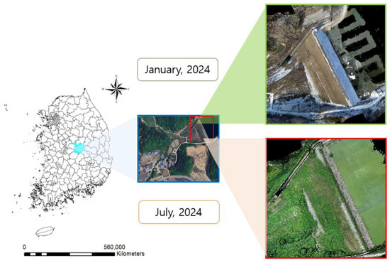
Figure 2. Research Area.

2.2.2. Survey Equipment

To establish an objective baseline for comparison, this study conducted both a VRS survey, GCP and check point (CP) survey across the entire site. For this task, a Trimble (Westminster, CO, USA) R8S high-precision satellite signal receiver and a Juno T41/5 PDA device were used for data collection and transmission (Table 1). The UAV platform employed was the Matrice 300 RTK, a rotary-wing model from DJI (Shenzhen, China). This aircraft provides stable flight performance through its real-time kinematic (RTK) capabilities and offers the advantage of supporting various sensor payloads. In particular, for LiDAR surveying, unlike photogrammetry, accurate GNSS positioning is required to construct point clouds and generate 3D spatial information. This requirement can be satisfied using either (RTK or post-processed kinematic (PPK) techniques during data acquisition and processing. Accordingly, to correct the UAV’s positional errors in real time during the LiDAR survey and ensure stable flight, a field-deployable single-baseline RTK unit, the DJI D-RTK 2 Mobile Station, was integrated into the system (Table 2) [26,27]. Unlike the VRS method, the RTK technique uses a single base station to correct the UAV’s position without an internet connection, which makes it more advantageous under field conditions with poor network communication. Furthermore, the DJI Zenmuse L1 sensor was used for LiDAR terrain mapping. This unit is fully compatible with the Matrice 300 RTK and is equipped with an RGB optical camera, enabling simultaneous LiDAR surveying and photogrammetry during a single UAV flight. Notably, the Zenmuse L1 integrates a Livox Avia LiDAR sensor, which measures distance using laser pulses with a wavelength of 905 nm. During the photogrammetric processing, the intrinsic parameters of the Zenmuse L1 RGB camera—including focal length, sensor size, and image resolution—were applied (Table 3) [28].

Table 1. Specification of Trimble R8s and Juno T41/5.

GNSS Data Receiver (VRS Survey)			GNSS Data Processor
Trimble R8s			Juno T41/5
Type		Specification	Type	Specification
Channels		$440 \mathrm{C}\mathrm{h}\mathrm{a}\mathrm{n}\mathrm{n}\mathrm{e}\mathrm{l}\mathrm{s}$	Operating System	Android 4.1 Jellybean
Weight		$3.8 \mathrm{k}\mathrm{g}$ (Including Battery)	Weight	$400 \mathrm{g}$
Satellite Signals (GPS)		L1C/A, LIC, L2C, L2E, L5	RAM	$512 \mathrm{M}\mathrm{B}$
Network-RTK	Horizontal	$8 \mathrm{m}\mathrm{m}$$+ 0.5 \mathrm{p}\mathrm{p}\mathrm{m}$ RMS	Storage	$8 \mathrm{G}\mathrm{B}$
	Vertical	$15 \mathrm{m}\mathrm{m}$$+ 0.5 \mathrm{p}\mathrm{p}\mathrm{m}$ RMS	Processor	$800 \mathrm{M}\mathrm{H}\mathrm{Z}$

Table 2. Specification of DJI Matrice 300 RTK and D-RTK 2 Mobile Station.

UAV		Single-Baseline RTK Station
Matrice 300 RTK		D-RTK 2 Mobile Station
Flight Altitude	≤7000 m	Satellite Signal (GPS)	L1, C/A, L2, L5
Flight Time	≤55 min	Positioning Precision (Single)	Vertical: 3.0 m
			Horizontal: 1.5 m
Hovering Accuracy (GPS)	Vertical: ±0.1 m	Positioning Precision (RTK)	Vertical: 2 cm + 1 ppm
	Horizontal: ±0.1 m		Horizontal: 1 cm + 1 ppm
RTK Positioning Accuracy	Vertical: 1.5 cm + 1 ppm	Size	168 × 168 × 1708 mm
	Horizontal: 1 cm + 1 ppm
Speed	≤17 m/s	Memory Volume	16 GB
Weight	3.6 kg (Excluding Battery)	Weight	5.7 kg (Excluding Tripod)
	6.3 kg (Including Battery)		8.1 kg (Including Tripod)

Table 3. Specification of DJI Zenmuse L1(RGB Optical camera, LiDAR).

Sensor (Platform)
Zenmuse L1
RGB Optical (Photogrammetry)		LiDAR
Category	Detail	Category	Detail
Resolution	3840 $\times$ 2160 Pixel	Measurement Accuracy	$3 \mathrm{c}\mathrm{m}$$/100 \mathrm{m}$
File Format	JPEG	Detection Range	$450 \mathrm{m}$
F-Stop	f/2.8~f/11	Scan Mode	Repeat/Non-Repeat Mode
FOV (Field Of View)	$95°$	FOV	Repeat	Vertical: $4.5°$
				Horizontal: $70.4°$
Focal Length	$8.8 \mathrm{m}\mathrm{m}$$/24 \mathrm{m}\mathrm{m}$		Non- Repeat	Vertical: $77.2°$
				Horizontal: $70.4°$
ISO	100	Number of Returns Wavelength	3 (Maximum)
			$905 \mathrm{n}\mathrm{m}$
Shutter Speed	1/2000-8 s (Mechanical)	Real-Time Point Cloud Coloring Modes	True Color; Coloring by Reflectivity; Coloring by Elevation
Effective Pixels	20 $\mathrm{M}\mathrm{P}$
Photo Size	4864 $\times$ 3648	Laser Safety	Class 1
Sensor Size	$1 \mathrm{i}\mathrm{n}\mathrm{c}\mathrm{h}$	Size	152 $\times$ 110 $\times$ 169 $\mathrm{m}\mathrm{m}$
Size	152 $\times$ 110 $\times$ 169 $\mathrm{m}\mathrm{m}$	Weight	930 $\pm$ 10 $\mathrm{g}$
Weight	930 $\pm$ 10 $\mathrm{g}$

2.3. VRS and GCPs Survey

The study site is a levee of an agricultural reservoir managed by the Korea Rural Community Corporation, a public institution in the Republic of Korea. Official DTM data and earthwork volume information for this area were not available. Therefore, to establish an objective reference standard for the research, a comprehensive VRS survey was conducted across the entire site (Figure 3). Therefore, unlike the UAV surveys, the VRS survey was conducted beforehand in mid-January 2024, when vegetation was minimal, and it applied the national geoid model KN-Geoid 18 (Korea National Geoid 18) and the projected coordinate system Korea 2000/Central Belt 2010 (EPSG:5186). The national geoid model KN-Geoid 18 was applied to convert ellipsoidal GNSS heights into orthometric heights, ensuring a consistent vertical reference for DTM generation and earthwork volume analysis. During the reference point measurements, the average number of tracked satellites exceeded 20, with a vertical precision of ±0.015 m and a horizontal precision of ±0.009 m. The position dilution of precision (PDOP) value was approximately 6 or less, satisfying the national geographic information institute (NGII) Notice No. 2015-2538: Regulations on Public Survey Procedures. In accordance with the same regulations, approximately 250 survey points were arranged in a grid pattern with an average spacing of 3 m, and each point location was measured for more than 10 s to ensure positional precision. However, in areas that were difficult to access or where depressions were present, field constraints caused the spacing between some points to exceed 3 m. The entire survey took approximately 4 h and 30 min to complete (Figure 3).

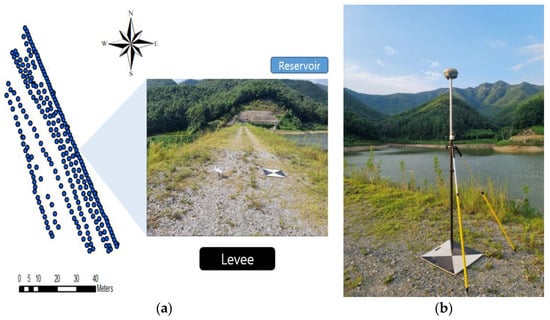
Figure 3. Data Acquisition: (a) Point Coordinates result of VRS (GNSS) Survey (Ground Truth), (b) GCPs Survey.

Additionally, to obtain correction coordinates for the georeferencing of the UAV photogrammetry and LiDAR data, GCPs were installed and measured prior to the UAV flights, all of which were conducted on the same day in July (Figure 3). Prior to the UAV operations, a total of eight control targets were evenly installed across the study area in locations that were clearly identifiable by the UAV camera, using black-and-white checkered aerial markers. Among them, Points 1, 2, 3, 7, and 8 were designated as GCPs and were used exclusively for georeferencing adjustment, whereas Points 4, 5, and 6 were designated as independent CPs for external accuracy evaluation. According to the UAV surveying regulations of the Republic of Korea (NGII Notice No. 2020-5670), control points must, in principle, be installed at a density of at least nine points per square kilometer. Similar studies conducted in areas of comparable size have also reported the use of fewer than ten control points [29,30]. The coordinates of all targets were acquired using the same VRS surveying method, with more than 25 tracked satellites and a PDOP value of 6 or less. The reported values of ±0.009 m (horizontal) and ±0.014 m (vertical) represent the internal precision indicated by the VRS receiver during measurement, rather than absolute positional accuracy, which was evaluated separately using the independent CPs. Installation and surveying required approximately 30 min due to dense vegetation and irregular rock formations.

2.4. Data Acquisition—UAV Photogrammetry

As photogrammetry is a passive remote sensing method that depends heavily on sunlight, there is potential for brightness errors and shadow-induced distortion. To mitigate this, the survey was conducted between 1:00 PM and 2:00 PM, when the solar altitude was highest, and under wind conditions below 1 m/s to minimize aircraft instability. Prior to the flight, a ground calibration was performed to calibrate the accelerometer, gyroscope, and compass, thereby minimizing potential data distortion. To ensure an adequate horizontal field of view and parallax, the flight parameters were set to the recommended standards of 70% front overlap and 60% side overlap. According to NGII Notice. No. 2020-5670, Regulations on Surveying Operations using Unmanned Aerial Vehicles in the Republic of Korea, the standard overlap for aerial imagery is set to 65% in the flight direction (Front overlap) and 60% between adjacent flight lines (Side overlap), although these values may be adjusted depending on the flight plan and specific project requirements. The resulting ground sampling distance (GSD) was approximately 0.02 m/pixel, which corresponds to the selected flight altitude and camera sensor specifications. The automated flight mission was completed in approximately 9 min (Figure 4 and Figure 5). The UAV flight altitude was fixed at 50 m, and the flight speed was maintained at 4 m/s to ensure consistent capture of object feature points across the images. A total of 210 high-resolution images were acquired during the survey.

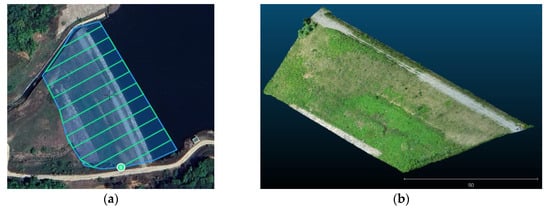
Figure 4. Terrain Data acquisition using UAV Photogrammetry: (a) Data Acquisition Route using UAV Photogrammetry (Ⓢ: Start point, Blue boundary: Survey area, Cyan line: Flight path), (b) Point cloud generated through UAV Photogrammetry (Scale unit: m).

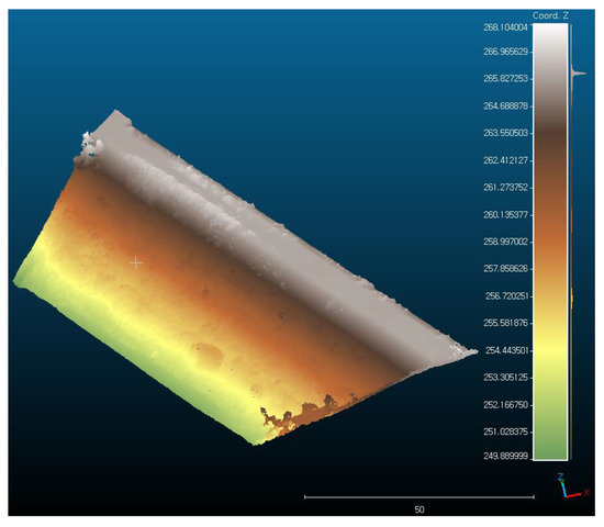
Figure 5. Three-dimensional Point Cloud Visualization Colored by Elevation (Scale unit: m)—UAV Photogrammetry.

2.5. Data Acquisition—UAV LiDAR

A LiDAR sensor is an active remote sensing instrument that determines range coordinates by emitting laser pulses toward a target and analyzing the time difference in the returning signals [31,32]. This technology generates a high-density three-dimensional point cloud from the collected data and, depending on the scanning method, can capture multiple returns from surfaces. Notably, some laser pulses can penetrate the upper vegetation canopy and reach the ground to produce additional returns, which is highly advantageous for acquiring terrain information beneath complex tree canopies. This makes LiDAR more effective for ground extraction in complex terrains compared with photogrammetry, which indirectly reconstructs surfaces by matching feature points across images. In this study, RGB imagery and LiDAR point cloud data were acquired using the DJI Zenmuse L1 system, which integrates an RGB camera for photogrammetry and a LiDAR sensor for point-cloud generation. The Zenmuse L1 has the capability to simultaneously record LiDAR point clouds and RGB images during flight. In this study, both the UAV LiDAR and photogrammetry surveys were conducted at the same site on the same day. Although they were performed in separate flight missions, environmental conditions such as lighting and weather remained largely consistent.

After completing the photogrammetric flight, a second flight was immediately conducted for LiDAR acquisition. A D-RTK 2 Mobile Station, a single-baseline RTK station, was used for real-time aircraft position correction. Additionally, an automated in-flight calibration was performed along the flight path, which is a standard procedure for the LiDAR sensor. The total flight time was approximately 14 min (Figure 6 and Figure 7). To generate a high-density point cloud, a repetitive scanning pattern and a laser pulse setting of approximately 200 pts/m² were applied, together with a triple-return configuration. The repetitive scanning approach surveys the same area multiple times, increasing the likelihood of capturing ground returns and improving the probability of acquiring terrain information obscured by upper-level vegetation. In contrast, a non-repetitive scanning method surveys the area only once, causing most laser pulses to be reflected by the upper vegetation canopy and resulting in an insufficient number of ground-reaching pulses, which can reduce the accuracy of DTM generation.

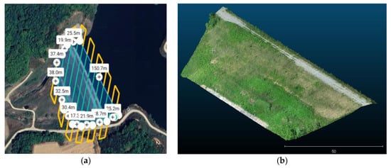
Figure 6. Terrain data acquisition using UAV LiDAR: (a) Data acquisition Route using UAV LiDAR (Blue boundary: Survey area, Cyan line: Flight path, Yellow line: Calibration segment), (b) Point cloud generated through UAV LiDAR (Scale unit: m).

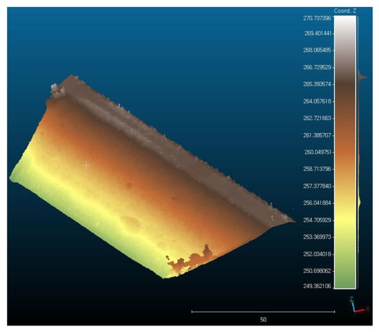
Figure 7. Three-dimensional Point Cloud Visualization Colored by Elevation (Scale unit: m)—UAV LiDAR.

2.6. Coordinate Adjustment of GCPs

In this study, point clouds of the target site were acquired using UAV photogrammetry and LiDAR sensors. In particular, a mobile RTK base station was installed on-site during the LiDAR survey to provide real-time position corrections and ensure UAV positional accuracy. However, the RTK method has a systematic limitation, as cumulative error increases with distance from the base station. Furthermore, unlike LiDAR, photogrammetry is an indirect reconstruction method that is highly susceptible to environmental conditions, making it prone to significant systematic errors if performed without GCPs correction. Specifically, in aerial imagery, the near-nadir viewing angle results in a narrow stereoscopic angle distribution and limited depth parallax, which tends to degrade reconstruction performance in the vertical (Z) direction. In contrast, the horizontal directions (X and Y) can maintain relatively high accuracy because sufficient parallax is secured between images. Indeed, previous studies have reported that when photogrammetry is performed without coordinate correction—such as GCP-based georeferencing—a “doming effect” can occur during the multi-view stereo (MVS) processing stage. This effect causes an excessive increase in altitude error, significantly reducing the reliability of the generated DTM [33].

The systematic characteristics of the photogrammetric data were examined through a residual analysis conducted at the GCP and CP locations. Before georeferencing adjustment, the photogrammetric model exhibited large residuals of 0.17 m in the X direction, 1.23 m in the Y direction, and 28.93 m in the Z direction at the five GCPs, indicating that substantial vertical bias was present in the initial model due to the challenging feature-extraction conditions of the site and the absence of RTK correction during image acquisition. To correct these offsets, georeferencing adjustment was performed using the five GCPs whose absolute coordinates were obtained from the VRS survey. After adjustment, the GCP residuals were reduced to 0.06 m, 0.07 m, and 0.03 m, demonstrating that the initial elevation inflation had been effectively eliminated (Table 4). The three independent CPs were subsequently used to evaluate the external accuracy of the adjusted photogrammetric model, and their residuals confirmed that the correction was applied successfully without overfitting to the GCPs. For the LiDAR dataset, georeferencing accuracy was assessed using the same eight VRS-derived GCP and CP coordinates. Because the LiDAR point cloud is generated directly by the sensor, the post-adjustment deviations measured at the CPs were treated as residuals rather than RMSE values. The resulting deviations 0.11 m, 0.06 m, and 0.06 m indicate stable accuracy within acceptable tolerance limits (Table 5).

Table 4. Result of Coordinates Adjustment between UAV Photogrammetry and GCPs (Unit: $\mathrm{m}$).

P.T No.	Control Points (VRS)			UAV Photogrammetry			Residual (Original)
	X	Y	Z	X	Y	Z	X	Y	Z
1	283,044.75	428,481.03	266.10	283,044.77	428,482.36	294.92	0.02	1.33	28.82
2	283,023.27	428,525.33	266.03	283,023.48	428,526.55	294.89	0.21	1.22	28.86
3	282,992.60	428,588.92	266.11	282,992.78	428,590.14	294.92	0.18	1.22	28.81
4	282,979.68	428,583.93	261.28	282,979.95	428,585.11	290.20	0.27	1.18	28.92
5	282,975.24	428,568.48	256.54	282,975.43	428,569.67	285.56	0.19	1.19	29.02
6	283,011.28	428,512.63	260.08	283,011.45	428,513.98	289.04	0.17	1.35	28.96
7	282,974.23	428,545.83	252.39	282,974.41	428,547.01	281.40	0.18	1.80	29.01
8	282,990.70	428,510.65	252.17	282,990.83	428,511.86	281.19	0.13	1.21	29.02
Total RMSE (Original)							0.17	1.23	28.93
Total RMSE (Adjustment)							0.06	0.07	0.03

Table 5. Result of Coordinates Adjustment between UAV LiDAR and GCPs (Unit: $\mathrm{m}$).

P.T No.	Control Points (VRS)			UAV LiDAR			Residual (Original)
	X	Y	Z	X	Y	Z	X	Y	Z
1	283,044.75	428,481.03	266.10	283,044.13	428,480.53	266.06	0.62	0.50	0.04
2	283,023.27	428,525.33	266.03	283,023.37	428,525.13	265.88	0.10	0.20	0.15
3	282,992.60	428,588.92	266.11	282,992.38	428,588.41	266.02	0.22	0.51	0.09
4	282,979.68	428,583.93	261.28	282,979.85	428,583.85	261.32	0.17	0.43	0.06
5	282,975.24	428,568.48	256.54	282,975.19	428,568.50	256.46	0.09	0.50	0.04
6	283,011.28	428,512.63	260.08	283,011.65	428,513.00	260.50	0.37	0.37	0.42
7	282,974.23	428,545.83	252.39	282,974.53	428,545.44	252.44	0.30	0.44	0.05
8	282,990.70	428,510.65	252.17	282,990.85	428,510.68	252.28	0.15	0.03	0.11
Total RMSE (Original)							0.30	0.40	0.17
Total RMSE (Adjustment)							0.11	0.06	0.06

To ensure precise target matching during georeferencing, the geometric centers of the checkered aerial targets were manually identified in both datasets. In photogrammetry, the exact center of each target was manually selected across all relevant images within Agisoft Metashape Professional (ver. 2.1.2) prior to the structure from motion (SfM) process. For LiDAR, the point clusters corresponding to each target were extracted in DJI Terra software (ver. 4.4.6), and their geometric centroids were manually selected to avoid positional bias. A noticeable difference was also observed in the time required for georeferencing. LiDAR correction was completed in approximately 30 min, whereas photogrammetry required about 2 h due to the repetitive matching of points (GCPs and CPs) across multiple images (Figure 8).

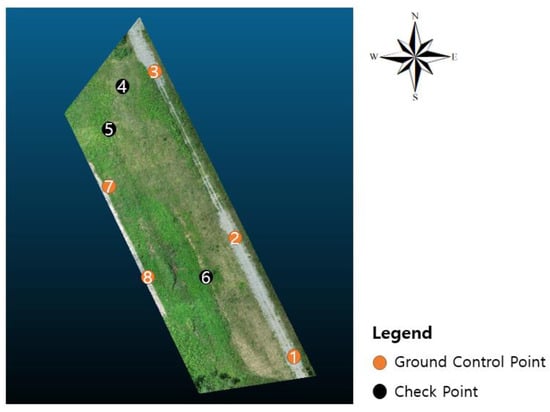
Figure 8. Location of Points (GCPs and CPs) installed at the Study site.

2.7. Data Sampling and Preprocessing

Although UAV photogrammetry and LiDAR acquire data through fundamentally different sensing mechanisms, both require a common set of preprocessing procedures. While both methods capture static terrain surfaces, photogrammetric point clouds are image-based reconstructions that rely on texture and visibility, making them more sensitive to lighting, surface reflectance, and occlusion. In contrast, LiDAR generates point clouds through active laser scanning, which can penetrate vegetation and provide more complete surface coverage in complex environments. Point cloud data from both photogrammetry and LiDAR exhibited high point density but also contained unnecessary points and various types of outliers generated by moving objects (e.g., people, birds, and vehicles), mismatches in image- or scan-based reconstruction, and vegetation-related misclassifications. These sources of noise increased data volume and reduced post-processing efficiency for both datasets. Therefore, an identical pre-processing workflow was applied to the corrected photogrammetry and LiDAR point clouds using Cloud Compare (ver. 2.13.2). First, a subsampling method with a point spacing of 0.01 m was used to reduce memory usage while preserving essential terrain features [31,34]. Subsequently, a k-nearest neighbors (k-NN) noise filter and a statistical outlier removal (SOR) filter were sequentially applied to remove points with abnormally low local density or abnormally large point-to-neighbor distances [35]. This process minimized anomalous data in both datasets and produced cleaned, high-quality point clouds under equivalent conditions, thereby ensuring a fair comparison of DTM generation and earthwork-volume estimation accuracy.

3. Application of Vegetation Removal Techniques

3.1. Overview of Vegetation Removal Techniques

In this study, the ground surface was extracted from terrain models constructed using two different UAV-based surveying methods. This was accomplished by applying three vegetation removal indices derived from RGB color information and a coordinate-based vegetation filtering algorithm. Numerous point cloud–based ground extraction techniques have been proposed in previous studies. Among them, Woebbecke et al. (1995) reviewed several vegetation indices that utilize color information to distinguish between vegetation and ground surfaces [36].

The vegetation indices adopted in this study are designed to effectively remove non-terrain points by mathematically emphasizing the spectral characteristics of vegetation—specifically, its high reflectance of green light and strong absorption of red light. Although UAV photogrammetry and LiDAR differ in their data acquisition methods and 3D model reconstruction principles, they share a common feature: both provide 8-bit (0–255) color information for the red (R), green (G), and blue (B) channels along with 3D coordinates. Based on this shared characteristic, a total of seven vegetation removal techniques were applied to both the photogrammetric and LiDAR datasets to compare their performance:

• Vegetation removal indices emphasizing the green channel: ExGR, GRVI, and VARI.
• Adaptive TIN (ATIN)-based ground extraction algorithm: Lasground (new), a TIN densification method implemented in LAStools, an open-source plugin for QGIS.
• Combined method: Application of the Lasground (new) algorithm to terrain data after the vegetation removal indices had been applied.

3.1.1. Excess Green Minus Red Index (ExGR)

The ExGR index is calculated by subtracting the excess red (ExR) index from the excess green (ExG) index. This method is designed to maximize the visible dominance of green within an image. Rather than simply measuring the proportion of green values in a given area, it quantifies how much greener a pixel is relative to the other color components—red and blue. This enables the effective separation of live green vegetation from soil, dry vegetation, and artificial objects Equation (1). The ExGR index has been widely applied in the agricultural sector, particularly for the precise detection of crop areas and the identification of weeds. It shows a distinct advantage in clearly delineating the boundary between vegetated and non-vegetated surfaces [37,38,39].

$$\begin{gathered} \mathrm{r}={\displaystyle \frac{Red}{Red+Green+Blue}}, g={\displaystyle \frac{Green}{Red+Green+Blue}}, b={\displaystyle \frac{Blue}{Red+Green+Blue}} \\ ExGR=\left(\right(2\ast g)-r-b)-\left(\right(1.4\ast r)-g) \end{gathered}$$

(1)

3.1.2. Green-Red Vegetation Index (GRVI)

The GRVI is one of the simplest and most intuitive vegetation indices. It is based on the fundamental principle of vegetation analysis that plants strongly reflect green light while absorbing red light, and it is calculated using only the difference between the values of the green and red channels Equation (2). Structurally, GRVI is analogous to a simplified form of the normalized difference vegetation index (NDVI), a widely used index for multispectral sensors, but adapted for the visible light spectrum (400–700 nm). Although GRVI is simple and computationally efficient, it is sensitive to lighting conditions and shadows. Therefore, it yields optimal results when applied to data captured under consistent illumination conditions [40].

$$GRVI={\displaystyle \frac{Green-Red}{Green+Red}}$$

(2)

3.1.3. Visible Atmospherically Resistant Index (VARI)

The VARI is a color-based vegetation index designed to minimize the effects of atmospheric conditions without requiring a NIR band Equation (3). VARI is specifically developed to exhibit enhanced resistance to atmospheric disturbances, thereby enabling more stable vegetation analysis. Its primary objective is to reduce the influence of light scattering caused by aerosols and water vapor in the atmosphere, which frequently occur during satellite imaging or UAV-based aerial photography. A key feature of VARI is its utilization of the blue channel to compensate for atmospheric effects while still being based on the spectral difference between the green and red channels. Consequently, VARI tends to produce more consistent results than other indices, even under variable lighting conditions or in areas with mild shadowing [41].

$$VARI={\displaystyle \frac{Green-Red}{Green+Red-Blue}}$$

(3)

3.1.4. QGIS LAStools Lasground (New) Algorithm

The Lasground (new) algorithm is an improved version of the original Lasground method, developed to enable stable ground surface extraction even in complex terrains containing both mountainous and urban features. This proprietary LAStools algorithm is based on a hierarchical, TIN-based surface estimation approach (the ATIN algorithm) [42], which selects initial ground candidates and then iteratively refines them to construct the final terrain model. Non-ground objects such as buildings and trees are progressively removed through a grid-based search. During this process, parameters such as terrain type (e.g., urban, mountain), pre-processing settings, and noise removal thresholds (Spike, Down Spike) can be flexibly adjusted, making the algorithm effective for both photogrammetry- and high-density LiDAR-based point cloud data (LAS format).

Leveraging these features, this study aimed to precisely detect fine-scale terrain undulations. To achieve this, the terrain type parameter was set to Wilderness, the pre-processing specification to hyper fine, and the grid (step) size to 1.0 m. In addition, Spike and Down Spike thresholds of 0.1 m were applied to remove noise points that were either sharply elevated or depressed below the surface, and an Offset value of 0.05 m was used to ensure surface continuity. Using a small grid size allows fine terrain variations to be more faithfully represented. However, excessively fine parameter tuning may cause the algorithm to misclassify ground points as vegetation or noise, resulting in the unintended removal of actual ground areas. Therefore, the parameters were optimized to maintain an appropriate balance between precision and stability [43,44].

3.2. Qualitative Comparison of Method (Visual Analysis)

3.2.1. RGB Vegetation Index Application—UAV Photogrammetry

Visual analysis revealed that areas classified as vegetation thresholds were effectively removed when the color indices were applied, resulting in an overall decrease in the average terrain elevation (Figure 9). In the graphs, colors closer to brown indicate higher elevation values, whereas colors closer to light green represent lower-elevation points (Figure 10). However, in the photogrammetry dataset, regions previously occupied by dense low-lying vegetation exhibited a shortage of ground points after vegetation removal (Figure 11). This occurred because the underlying ground surface had not been sufficiently captured, leaving gaps once the vegetation was removed. Notably, this issue occurred despite meeting the national minimum overlap standards and is attributed to the inherent structural limitation of photogrammetry—a passive, optical sensing technique that cannot directly observe the ground beneath shallow grass or understory vegetation. Furthermore, the removal of some boundary ground points together with vegetation during the filtering process contributed to the expansion of these gaps.

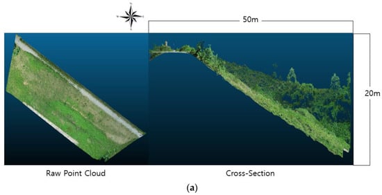
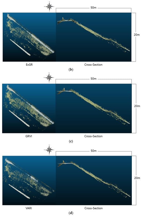
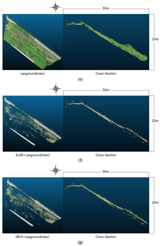
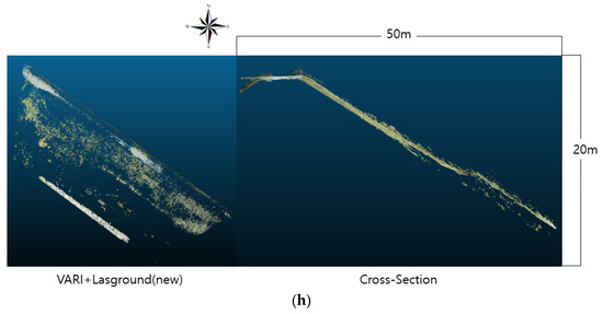
Figure 9. Vegetation Removal results and Cross-Sectional visualization (Width: 50 m, Elevation Difference: 20 m) of Point cloud—UAV Photogrammetry: (a) Raw Point Cloud, (b) ExGR, (c) GRVI, (d) VARI, (e) Lasground (new), (f) ExGR + Lasground (new), (g) GRVI + Lasground (new), (h) VARI + Lasground (new).

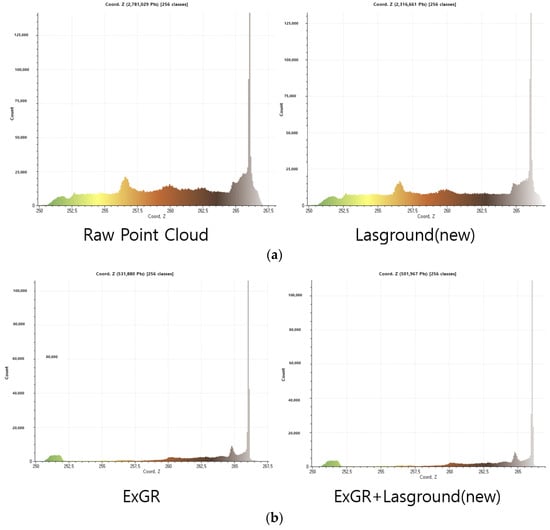
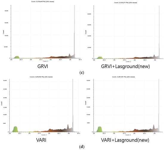
Figure 10. Histogram of Elevation Distribution for Filtered Point Clouds –UAV Photogrammetry: (a) Raw Point Cloud & Lasground (new), (b) ExGR & ExGR + Lasground (new), (c) GRVI & GRVI + Lasground (new), (d) VARI & VARI + Lasground (new).

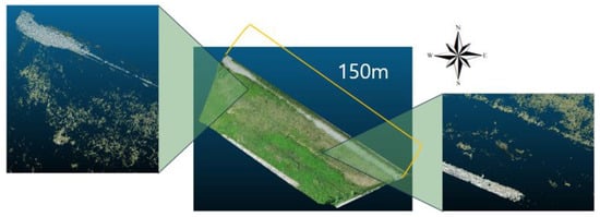
Figure 11. Deficiency of ground points in densely vegetated regions following the application of vegetation removal indices (UAV Photogrammetry).

In terms of the performance of each index, GRVI retained the greatest number of points and most stably preserved the continuity of the terrain; however, gaps still appeared on the ground surface beneath tree canopies. The ExGR index retained more points than VARI but did not entirely remove vegetation clusters, which tended to remain as residual noise. In contrast, VARI, despite retaining the fewest points, exhibited the best performance in removing aerial noise. Nevertheless, it sometimes misidentified and unnecessarily removed yellowish surfaces or dry grass, with particularly significant point loss over gray gravel and rocky areas. This phenomenon is associated with the systematic limitations of photogrammetry, which is highly sensitive to external lighting conditions and shadows. Although VARI, like the other indices, utilizes green contrast, its structure—where the blue component is subtracted in the denominator renders it more susceptible to atmospheric and shadow effects. This can lead to unstable index values and excessive removal of white-to-gray surfaces, which are misinterpreted as vegetation due to spectral similarity with green reflectance, even when representing actual ground surfaces. Specifically, because the RGB distributions of gravel and rock points within the point cloud are similar, the balance between the numerator and denominator is easily distorted (Figure 12). This caused actual ground surfaces to be assigned VARI values above the threshold and consequently removed. In contrast, the simple structure of GRVI (reflecting only green and red components) and the balanced, normalized structure of ExGR prevented extreme value distortion, even in gravel and rocky areas. Owing to this stability, instances of actual ground surfaces being misclassified as vegetation were rare, and gravel and rock zones were generally maintained with neutral index values, thereby preserving ground information.

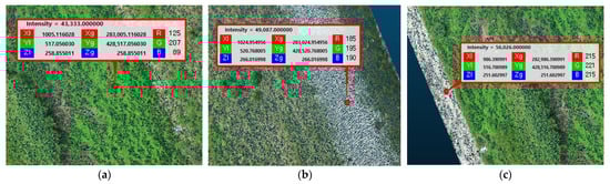
Figure 12. Distribution of RGB information by land cover (vegetation, gravel, rock)—UAV Photogrammetry: (a) Vegetation (Shrubs), (b) Gravel Field, (c) Rocky Area.

3.2.2. Lasground (New) Algorithm Application—UAV Photogrammetry

When the Lasground (new) algorithm, a ground extraction method based on terrain geometry was applied independently, it effectively removed protruding vegetation and isolated outlier points. However, in areas where dense, low-altitude vegetation obscured the surface during data acquisition, only a limited number of ground observations were available in the original photogrammetric point cloud. As a result, the algorithm could not classify ground points in these occluded regions, leading to gaps that reflect the absence of ground observations rather than the removal of existing ground points. In addition, dense vegetation in the upper part of the site was not fully filtered, indicating that unresolved vegetation could still contribute to elevation inconsistencies during subsequent terrain-model generation.

In contrast, when the color indices were combined with Lasground (new), the protruding noise that had remained when the indices were applied alone was also removed, resulting in an overall improvement in extraction performance. However, this combined approach also tended to smooth the average elevation because some near-ground points that had been incompletely reconstructed beneath low vegetation were removed together with the vegetation, and data gaps persisted in areas where ground observations had been insufficient during acquisition. Specifically, the combination with the ExGR index was effective in removing noise from objects located over gravel surfaces. The combination with GRVI eliminated not only protruding vegetation but also residual aerial noise, achieving the most complete ground reconstruction in the photogrammetry dataset. The combination with VARI partially compensated for the over-filtering problem observed when it was used alone, providing stable performance without additional data loss. In summary, applying the color indices alone exhibited distinct strengths and trade-offs between ground preservation and noise removal. Integrating them with the Lasground (new) algorithm mitigated these limitations, enabling more stable and continuous ground reconstruction. This combined approach also effectively removed residual aerial noise, thereby improving the overall quality of the ground extraction (Figure 9 and Figure 10).

3.2.3. RGB Vegetation Index Application—UAV LiDAR

Unlike with photogrammetry, the LiDAR data showed clear and consistent improvements in preserving ground information beneath the canopy and in suppressing noise generation in this particular dataset (Figure 13). The same color scale as used in the photogrammetry-based analysis was applied, where brownish colors indicate higher elevations and light green colors represent lower-elevation points (Figure 14). It should be noted, however, that these findings reflect the characteristics of this specific landscape and vegetation structure, and therefore should not be generalized to all terrain types or dense vegetation conditions. This means that some ground points were retained even under dense vegetation clusters, providing a stronger statistical basis for increasing the reliability of the subsequent ground reconstruction process (Figure 15). When ExGR index was applied, some canopies in dense vegetation areas were not completely removed, leaving some points floating. However, compared to photogrammetry, significantly more ground points were preserved, thereby maintaining the continuity of the terrain. The results from GRVI showed a similar trend, but in addition to preserving the ground beneath the canopy, it also removed most of the yellow and blue-hued objects on the gravel terrain. Furthermore, there was relatively little isolated aerial noise remaining after vegetation removal, which clearly highlighted the difference in filtering performance between LiDAR and photogrammetry. The difference between the two survey methods was particularly pronounced with the VARI. In the photogrammetry data, gravel and rock areas were excessively removed, resulting in the loss of valid ground observation in the point cloud and the creation of unintended gaps. In the LiDAR data, however, this issue was largely absent, aside from a few points along the edges. This is because, unlike photogrammetry, LiDAR data is fundamentally based on 3D coordinates acquired from laser pulses, with color being overlaid in post-processing. Therefore, VARI only uses color as a supplementary aid to classify points; it does not delete the underlying coordinates that form the basis of the terrain (Figure 16). As a result, even if a classification error occurred, it did not lead to terrain loss, allowing the exposed ground surface to be stably preserved. Additionally, the gravel area located in the upper part of the site, where ground loss occurred, was extracted based on the same coordinate domain, and the proportion of points with VARI values greater than 0.1 (classified as vegetation) was calculated (Figure 17). As a result, approximately 20.4% of the total points in the photogrammetry dataset had values greater than 0.1, whereas the LiDAR dataset showed only 4.3%, representing a reduction by a factor of about 4.8 times. Notably, although the LiDAR data contained a larger total number of points in the gravel area, the number of points exceeding 0.1 was approximately 4.3 times lower than in the photogrammetry data (Table 6). This confirms that point loss in the gravel area occurred significantly more frequently in photogrammetry than in LiDAR. However, some aerial vegetation noise that had been removed from the photogrammetry data tended to remain in the LiDAR data, and its performance in removing objects over gravel was on a similar level to that of GRVI. In summary, for all color indices, LiDAR demonstrated superior performance over photogrammetry in preserving ground information beneath the canopy and suppressing noise. In particular, the VARI was less sensitive to external lighting conditions and shadows than photogrammetry, effectively preventing excessive loss of ground areas. However, it should be noted that these results reflect the vegetation characteristics of the study site, where the density of ground-blocking vegetation was not high enough to completely prevent laser penetration. In vegetation communities with extremely dense, tall, or matted structures—such as tightly packed grasses or shrubs—LiDAR may also fail to obtain ground returns, resulting in local voids.

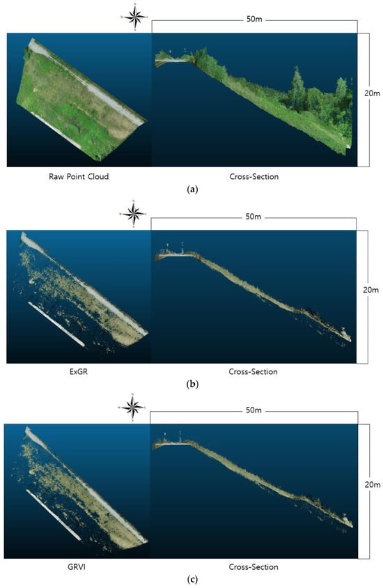
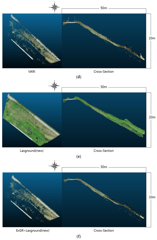
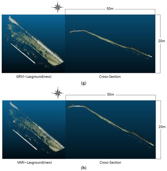
Figure 13. Vegetation Removal results and Cross-Sectional visualization (Width: 50 m, Elevation Difference: 20 m) of Point Cloud—UAV LiDAR: (a) Raw Point Cloud, (b) ExGR, (c) GRVI, (d) VARI, (e) Lasground (new), (f) ExGR + Lasground (new), (g) GRVI + Lasground (new), (h) VARI + Lasground (new).

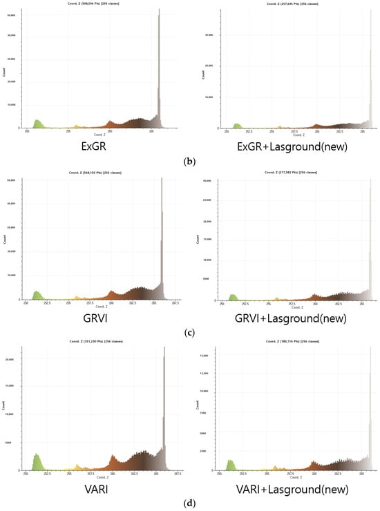
Figure 14. Histogram of Elevation Distribution for Filtered Point Clouds –UAV LiDAR: (a) Raw Point Cloud & Lasground (new), (b) ExGR & ExGR + Lasground (new), (c) GRVI & GRVI + Lasground (new), (d) VARI & VARI + Lasground (new).

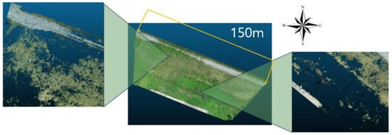
Figure 15. Preserved Ground points in dense Vegetation enabled by Multi Return and Repetitive Scan mode (UAV LiDAR).

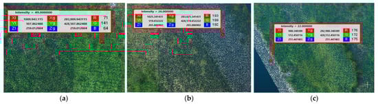
Figure 16. Distribution of RGB information by land cover (vegetation, gravel, rock)—UAV LiDAR: (a) Vegetation (Shrubs), (b) Gravel Field, (c) Rocky Area.

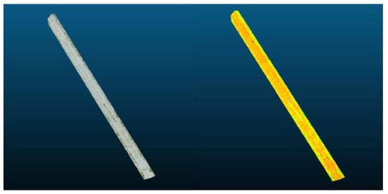
Figure 17. Point cloud extraction of gravel areas in the same site based on UAV photogrammetry and LiDAR data.

Table 6. Comparison of the proportion of points classified as vegetation (VARI $\ge$ 0.1) in the gravel area between UAV photogrammetry and LiDAR data.

Category	UAV Photogrammetry	UAV LiDAR
Number of Points (Total)	102,227 pts	114,162 pts
$\mathrm{VARI} \mathrm{value} \ge$ 0.1	20,799 pts	4880 pts
Ratio	20.35%	4.27%

3.2.4. Lasground (New) Algorithm Application—UAV LiDAR

When the Lasground (new) algorithm was applied alone, some areas exhibited coordinate voids due to a shortage of classified ground points, and dense low-lying vegetation remained partially unremoved (Figure 16 and Figure 17). While the algorithm effectively eliminated most localized protruding vegetation, the retained near-ground vegetation points produced a discontinuous, DSM-like pattern rather than a continuous bare-earth surface. Therefore, the resulting surface does not represent a complete DTM but instead approximates the terrain with residual low vegetation remaining. In the comparison between the two surveying methods, residual floating noise in the vegetation-removed areas was largely absent. However, photogrammetry exhibited limitations in removing vegetation from gravel zones, whereas LiDAR effectively eliminated most of it within the same regions. Notably, in the LiDAR dataset, a certain proportion of ground points was retained even after the application of Lasground (new), which mitigated coordinate voids in the filtered sections and ensured a stable dataset for ground reconstruction. Performance further improved when the color indices were combined with Lasground (new). The ExGR combination enabled stable reconstruction by removing objects that had been missed when it was applied independently, while the GRVI combination improved ground continuity by eliminating sporadically distributed vegetation. In contrast, the VARI combination was effective in removing protruding vegetation but resulted in partial ground loss, producing the lowest number of preserved ground points among the LiDAR-based combined techniques.

Overall, LiDAR demonstrated superior performance compared with photogrammetry. When Lasground (new) was applied alone, it was effective in removing localized vegetation but exhibited limitations in processing densely vegetated areas. However, when the data were pre-filtered using a color index prior to applying Lasground (new), dense vegetation and noise were effectively suppressed without compromising the underlying ground information. Therefore, a two-step procedure—first applying a color index to remove protruding vegetation and then applying Lasground (new)—is considered the most appropriate strategy in terms of vegetation-removal efficiency and the mitigation of noise effects. However, in areas where low-lying vegetation is tightly attached to the ground surface, the LiDAR laser cannot fully penetrate to the terrain, resulting in only partial ground-point retrieval and the formation of local voids in the terrain.

3.3. Estimation of Terrain Gaps—Kriging Interpolation Method

The Kriging interpolation method is a statistics-based geospatial interpolation technique that predicts values at data-sparse locations based on spatial correlation. It simultaneously calculates prediction errors, allowing for a quantitative assessment of the reliability of the results [45]. Unlike the inverse distance weighting (IDW) method, which considers only distance, Kriging determines weights using a variogram model that represents the spatial variability among observed values Equation (4). This approach minimizes estimation bias while also providing the estimation variance, thereby enabling simultaneous acquisition of both the interpolation result and its associated uncertainty information.

In this study, the Kriging interpolation function in Cloud Compare was used to estimate terrain elevations at unmeasured locations based on the extracted ground points, using a grid spacing of 0.05 m. This procedure provided the foundation for the subsequent DTM-generation step. Although Kriging enables the statistical estimation of 3D coordinates in data-missing areas and helps maintain spatial continuity, the interpolated values remain predictions. Therefore, the reliability of the resulting DTM is still strongly dependent on the accuracy and spatial distribution of the surrounding ground points—particularly in densely vegetated areas where ground observations were limited.

$$\begin{gathered} \gamma \left(h\right)={\displaystyle \frac{1}{2N\left(h\right)}}\sum _{i=1}^{N\left(h\right)}{\left(Z\right(s_i)-Z(s_i+h\left)\right)}^2 \\ {Z}^{*}\left(s_0\right)=\sum _{i=1}^n{\lambda }_{i}Z\left(s_i\right) \end{gathered}$$

(4)

4. Results and Discussion

4.1. Accuracy Assessment of DTM Generation—UAV Photogrammetry

To quantitatively evaluate the accuracy of the DTMs generated using various ground-extraction techniques applied to the UAV photogrammetry–derived point cloud, the resulting DTMs were compared with the VRS reference survey. Several error metrics were calculated for the accuracy assessment, including the RMSE, MAE, and the mean of height differences. Among these, RMSE was used as the primary indicator, while the remaining metrics served as supplementary measures of accuracy Equations (5)–(7).

Before presenting the DTM accuracy results, it is clarified that all datasets used in this analysis were corrected using GCP-based georeferencing prior to the accuracy assessment. In this context, the RMSE values reported in this section primarily reflect areas containing vegetation, while in bare ground areas acquired in January 2024, the RMSE for UAV photogrammetry was approximately 0.1469 m, indicating a relatively low level of error. According to the DTM accuracy analysis, the initial unfiltered dataset exhibited an RMSE of approximately 0.4074 m after GCP-based georeferencing. The initial RMSE reported in this section is not intended to represent standard or recommended practice but is used solely as a reference baseline for quantitatively comparing the relative effects of vegetation-removal techniques applied under identical georeferencing conditions. When individual vegetation-removal techniques were applied, the GRVI showed the best performance, yielding an RMSE of 0.2727 m. In addition, the ExGR (0.2824 m) and VARI (0.2912 m) indices also demonstrated improvements of more than 0.11 m compared to the initial unfiltered dataset (Table 7).

Table 7. Comparison of DTM Accuracy Values Generated based on UAV Photogrammetry (Reference: VRS Survey Data).

UAV Photogrammetry
Indices (Techniques)	Height Difference (m)				RMSE (m)	MAE (m)
	Max	Min	Mean	St. Dev
Raw Point Cloud	2.9749	−0.3226	0.2662	0.3085	0.4074	0.2881
ExGR	1.1408	−0.9156	0.0849	0.2139	0.2824	0.2385
GRVI	1.1984	−1.0968	−0.1603	0.2393	0.2727	0.2264
VARI	1.0606	−1.0968	−0.2010	0.2215	0.2912	0.2439
Lasground (new)	2.0395	−0.8681	0.1634	0.3144	0.3253	0.2364
ExGR + Lasground (new)	1.1242	−0.7666	−0.0075	0.1792	0.1793	0.1269
GRVI + Lasground (new)	1.1209	0.8142	−0.0869	0.1821	0.2017	0.1465
VARI + Lasground (new)	1.1086	−0.8165	−0.0904	0.1804	0.2018	0.1471

In contrast, the Lasground (new) algorithm, which primarily relies on geometric coordinate information, resulted in an RMSE of 0.3253 m, indicating lower performance than the color-index-based approaches. This outcome likely reflects the relatively limited vertical accuracy of the photogrammetry dataset and the insufficient observation of ground surfaces beneath the canopy during acquisition, which constrained the classification performance of Lasground (new) under the applied parameters. Nevertheless, residual noise and vegetation that were not removed by the color indices alone were further suppressed when combined with Lasground (new), resulting in an overall improvement in accuracy. Among the combined methods, the ExGR + Lasground (new) configuration produced the lowest RMSE of 0.1793 m under the conditions of this study. The GRVI and VARI combinations also showed noticeable improvements, recording RMSE values of 0.2017 m and 0.2018 m, respectively—an enhancement of more than 0.08 m—although the difference between the two was not statistically significant. These performance differences appear to be associated with the mathematical structure and inherent characteristics of each color index. ExGR distinguishes soil from vegetation relatively clearly by subtracting the excess red component from the excess green component. In contrast, VARI was originally developed to correct atmospheric scattering effects in satellite imagery using the blue channel. However, in low-altitude UAV imagery, atmospheric effects are comparatively minor, and thus the expected correction effect of VARI may not be fully realized, which may account for its slightly lower performance. In addition, partial loss of ground points, including those in gravel-dominated areas, occurred during the filtering process, which likely affected the quality of subsequent interpolation and DTM construction. These differences may vary depending on acquisition conditions, spectral characteristics, and the radiometric calibration of the sensor; therefore, careful interpretation of the results is necessary.

$$Height Difference Mean={\displaystyle \frac{1}{n}}\sum _{i=1}^n(Z_{DEM,i}-Z_{ref,i})$$

(5)

$$RMSE=\sqrt{{\displaystyle \frac{1}{n}}\sum _{i=1}^n{\left(Z_{DEM,i}-Z_{ref,i}\right)}^2}$$

(6)

$$MAE={\displaystyle \frac{1}{n}}\sum _{i=1}^n\left|Z_{DEM,i}-Z_{ref,i}\right|$$

(7)

4.2. Accuracy Assessment of DTM Generation—UAV LiDAR

The initial RMSE of the UAV LiDAR point cloud was approximately 0.3117 m (Table 8). A substantial portion of this deviation was attributable to the vegetation conditions present at the time of the survey. Field observations and survey photographs indicated that the vegetation primarily consisted of low grass and shrubs; however, in several areas, the plants formed dense and spatially continuous clusters that partially obstructed the laser pulses. This obstruction limited the number of valid ground returns and contributed to localized elevation uncertainties. In contrast, over bare ground areas, the RMSE of the UAV LiDAR data was approximately 0.0971 m, indicating reduced elevation uncertainty in the absence of vegetation. Furthermore, the GNSS checkpoints collected during the GCP and CP surveys were measured using a survey pole, allowing the antenna to be positioned well above the vegetation canopy and thus unaffected by signal obstruction caused by vegetation height.

Table 8. Comparison of DTM Accuracy Values Generated based on UAV LiDAR (Reference: VRS Survey Data).

UAV LiDAR
Indices (Techniques)	Height Difference (m)				RMSE (m)	MAE (m)
	Max	Min	Mean	St. Dev
Raw Point Cloud	2.3925	−0.4453	0.1125	0.2784	0.3117	0.2088
ExGR	2.2450	−0.9365	0.1115	0.2073	0.2354	0.1643
GRVI	2.0573	−0.6845	0.0549	0.1242	0.1913	0.1242
VARI	1.7992	−0.6339	0.0275	0.1787	0.1808	0.1198
Lasground (new)	2.1750	−0.3577	0.0810	0.1542	0.2322	0.1542
ExGR + Lasground (new)	1.4328	−0.3715	0.0377	0.1104	0.1674	0.1104
GRVI + Lasground (new)	1.4016	−0.5111	−0.0194	0.1098	0.1652	0.1098
VARI + Lasground (new)	1.3871	−0.6871	−0.0040	0.1132	0.1649	0.1132

When individual vegetation-removal techniques were applied to the LiDAR dataset, the resulting RMSE values ranged from 0.1808 m (VARI) to 0.2354 m (ExGR), with Lasground (new) yielding 0.2322 m. Although these results represent some improvement compared with the unfiltered LiDAR dataset, they should not be interpreted as evidence of high absolute accuracy. However, when the color indices were combined with the Lasground (new) algorithm, the RMSE values for VARI, GRVI, and ExGR converged to approximately 0.16–0.17 m, showing consistent relative improvements over their single applications. In particular, ExGR—previously the lowest-performing index—showed substantial improvement from 0.2354 m to 0.1674 m when combined with Lasground (new), demonstrating that this pairing was highly effective. GRVI exhibited stable performance in both the photogrammetry and LiDAR datasets, primarily due to its simple formulation based on the relative reflectance of green and red wavelengths, which allows it to effectively capture the spectral characteristics of vegetation while being less sensitive to variations in data acquisition conditions. Nonetheless, even under similar environmental settings, surfaces that appear visually similar produced noticeably different index values between photogrammetry and LiDAR. This difference arises from the fundamentally different ways in which RGB information is captured and radiometrically represented by the two systems.

For both datasets, combining a color index with Lasground (new) consistently enhanced the removal of protruding vegetation and improved the reconstruction of local terrain patterns. Although LiDAR generally exhibited smaller vertical deviations than photogrammetry when color indices were applied alone, the addition of Lasground (new) narrowed the differences between the two methods, resulting in no large RMSE distinctions. Therefore, the relative advantage of LiDAR observed in this study should be interpreted as increased robustness under conditions of dense, low vegetation, rather than as evidence of superior absolute accuracy. Residual uncertainty caused by vegetation occlusion remained in both datasets and should be considered when interpreting the results.

4.3. Accuracy Assessment of Earthwork Volume Calculation—UAV Photogrammetry

Earthwork volume is a key metric indirectly influenced by the quality of DTM and TIN models Equation (8), and it serves as one of the final performance indicators for verifying the accuracy of ground surface restoration [46]. The initial UAV photogrammetry-based point cloud resulted in an overestimation of approximately 5004.10 m³ compared to the reference data, showing an accuracy of 109.4% (Table 9). When applying single vegetation removal techniques, the calculated excess earthwork volume ranged from approximately 1900 m³ to 2600 m³ compared to the GNSS reference data. VARI showed 104.5% accuracy, while the ExGR index and GRVI demonstrated similar improvements, both at approximately 103.7% accuracy. The standalone application of Lasground (new) also recorded a result of 104.9%, showing performance comparable to the standalone application of GRVI.

Table 9. Comparison of Earthwork Volume Estimation Result Calculated based on UAV Photogrammetry (Reference: VRS Survey Data).

UAV Photogrammetry
Indices (Techniques)	Area (${\mathbf{m}}^2$)		Earthwork Volume (${\mathbf{m}}^3$)	Earthwork Volume Difference (${\mathbf{m}}^3$)	Total Earthwork Volume Accuracy (%)
	2D	3D
VRS (Ground Truth)	3680.37	4022.78	53,179.70	0.00	100.0
Raw Point Cloud	3671.79	4114.78	58,183.83	5004.13	109.4
ExGR	3668.25	4118.62	55,125.38	1945.68	103.7
GRVI	3676.14	4162.21	55,125.39	1945.69	103.7
VARI	3676.14	4204.09	55,570.56	2390.86	104.5
Lasground (new)	3676.50	4343.49	55,763.62	2583.92	104.9
ExGR + Lasground (new)	3671.09	4033.26	53,651.98	472.28	100.9
GRVI + Lasground (new)	3673.47	4036.20	53,577.92	398.22	100.7
VARI + Lasground (new)	3669.05	4027.12	53,999.27	819.57	101.5

In contrast, when color indices were combined with Lasground (new), the accuracy improved significantly compared to the previously applied methods. This improvement was due to the effective removal of elevation distortion caused by residual vegetation and unnecessary noise. Specifically, GRVI achieved an accuracy of approximately 100.7%, resulting in only 398.22 m³ of excess volume compared to the reference data, marking the best result among the photogrammetry-based techniques. The ExGR index also achieved 100.9% accuracy with 472.28 m³ of residual volume, successfully reducing the error margin to within 1% of the reference. VARI resulted in 819.57 m³ of residual volume and an accuracy of 101.5%, a 3% improvement compared to its standalone application. These results demonstrate that a hybrid method first removing vegetation using color indices and then complementarily processing remaining vegetation and other noise with Lasground (new) can efficiently reduce the overestimation inherent in the photogrammetry-based earthwork volume calculation process.

$$\begin{gathered} V_{Fill}=\sum _{i=1}^n\left(Z_i-Z_{ref}\right)·A_i, for Z_i<Z_{ref} \\ {V}_{Cut}=\sum _{i=1}^n\left(Z_i-Z_{ref}\right)·A_i, for Z_i>Z_{ref} \end{gathered}$$

(8)

$$V_{Total}=V_{Fill}+V_{Cut}$$

4.4. Accuracy Assessment of Earthwork Volume Calculation—UAV LiDAR

The initial UAV LiDAR-derived point cloud exhibited an overestimation trend, with an accuracy of approximately 108.1% compared with the reference. However, the overall accuracy improved after the application of vegetation-removal techniques (Table 10). This demonstrates that while UAV LiDAR inherently provides stable ground information, its performance can be further enhanced when combined with appropriate filtering methods.

Table 10. Comparison of Earthwork Volume Estimation Result Calculated based on UAV LiDAR (Reference: VRS Survey Data).

UAV LiDAR
Indices (Techniques)	Area (${\mathbf{m}}^2$)		Earthwork Volume (${\mathbf{m}}^3$)	Earthwork Volume Difference (${\mathbf{m}}^3$)	Total Earthwork Volume Accuracy (%)
	2D	3D
VRS (Ground Truth)	3680.37	4022.78	53,179.70	0.00	100.0
Raw Point Cloud	3676.95	4189.32	57,497.57	4299.87	108.1
ExGR	3679.48	4099.87	54,005.12	825.42	101.6
GRVI	3680.50	4101.00	55,043.26	1863.56	103.5
VARI	3676.63	4091.57	54,785.74	1606.04	103.0
Lasground (new)	3677.26	4100.57	55,380.26	2200.56	104.1
ExGR + Lasground (new)	3678.83	4043.98	53,337.81	158.11	100.3
GRVI + Lasground (new)	3679.84	4043.58	53,637.85	458.15	100.9
VARI + Lasground (new)	3679.88	4044.47	53,554.92	375.22	100.7

When single techniques were applied, ExGR showed the lowest Accuracy of Earthwork Volume calculation among the color indices (101.6%), while VARI and GRVI recorded 103.0% and 103.5%, respectively. In contrast, Lasground (new) exhibited a higher deviation (104.1%). This tendency appears to be consistent with the limited ground penetration observed in dense canopy areas and with the presence of some low-altitude vegetation points that were not fully removed or were misclassified under the applied parameter settings.

When the color indices were combined with Lasground (new), a further improvement in performance was observed. The combination with the ExGR index reduced the error by approximately 667.3 m³ compared with its single application, achieving an accuracy of 100.3% and yielding the best overall result. The combinations with VARI and GRVI also converged within a 1% error margin, with accuracies of 100.7% and 100.9%, respectively. In summary, for both surveying methods, integrating color-index filtering with Lasground (new) improved the accuracy of earthwork volume calculations, reducing the error margin to approximately 1%. When this combined filtering approach was applied, the LiDAR data consistently achieved errors below 1% under all conditions, demonstrating more stable and reliable performance than photogrammetry. Therefore, as the quantitative quality of the DTM improves, the accuracy of earthwork volume estimation increases proportionally. In practice, LiDAR is generally more advantageous for obtaining reliable results, whereas photogrammetry—given its operational efficiency remains a practical alternative or complementary tool under budgetary or environmental constraints.

5. Conclusions

To acquire data accurately reflecting terrain undulations, this study first obtained reference data through a Virtual Reference Station (VRS) GNSS survey conducted in winter, when vegetation was minimal. Subsequently, during the peak vegetation period, the same area was surveyed using a UAV equipped with a LiDAR sensor and an integrated RGB camera, with positional accuracy corrected via a GCP survey. After vegetation removal, only the remaining ground-classified points were used for Kriging interpolation, and the final DTM and TIN models were generated from this ground-only dataset. The results revealed a consistent trend for both surveying methods: applying the geometry-based Lasground (new) algorithm in combination with a color-based index improved both DTM quality and earthwork-volume accuracy. In the DTM accuracy assessment, the ExGR + Lasground (new) combination produced the best result for photogrammetry (RMSE = 0.1793 m). For LiDAR, the combinations of Lasground (new) with VARI, GRVI, and ExGR yielded similarly high accuracy (RMSE = 0.1649 m, 0.1652 m, and 0.1674 m, respectively). In the earthwork-volume calculation, the ExGR + Lasground (new) combination also performed best for both datasets, although the magnitude of error differed slightly between methods (≈0.9% for photogrammetry and ≈0.3% for LiDAR). These findings indicate that DTM quality is partially correlated with earthwork-volume accuracy and that, within the specific vegetation and terrain conditions of this study site, LiDAR provided somewhat more consistent terrain representation than photogrammetry. However, the observed vertical RMSE values for both UAV-based datasets (approximately 0.16–0.18 m) remain substantially higher than the centimeter-level accuracy achieved by the VRS reference survey. This underscores the inherent limitations of UAV-based reconstruction when used as a stand-alone source of ground-truth data. Although the combined filtering approach reduced vegetation-induced distortion and stabilized the terrain pattern, the absolute accuracy gap between UAV-derived DTMs and VRS measurements must be acknowledged when assessing the practical applicability of the results. Nevertheless, the performance of photogrammetry (RMSE = 0.1793 m and earthwork accuracy = 100.9%, with up to 100.7% achievable) was only marginally inferior to that of LiDAR. Therefore, LiDAR is recommended as the primary method for applications requiring higher robustness in dense vegetation, while photogrammetry, given its operational efficiency, remains a practical and cost-effective alternative under equipment or budget limitations.

Previous research has primarily focused on evaluating DTM quality after vegetation removal using a single survey method, with limited attempts to link those results to earthwork-volume accuracy for assessing practical applicability. This study distinguishes itself by directly comparing UAV photogrammetry and LiDAR in densely vegetated terrain and quantitatively analyzing the interrelationships among filtering performance, DTM quality, and earthwork-volume estimation accuracy. Although VRS surveying remains the most reliable method for establishing absolute ground truth, the findings of this study show that UAV-based techniques can provide useful supplementary data when field access or seasonal conditions restrict the ability to obtain sufficiently dense VRS measurements. In this sense, UAV observations function as a complementary, rather than a substitutive, source of terrain information in remote-sensing and construction-surveying applications.

Future work will extend beyond nadir-only surveys to include multi-angle photogrammetry and LiDAR acquisitions, analyzing their effects on DTM quality and the geometric characteristics of each method. Additional comparisons between interpolation methods—such as IDW and Spline—against Kriging will also be conducted to determine the optimal interpolation technique for different terrain types, thereby contributing to further improvements in DTM quality. Finally, additional seasonal validation is required during periods such as autumn, when the structural and color characteristics of vegetation change. By examining how vegetation-removal performance varies with seasonal differences in vegetation density and spectral reflectance, this research can establish seasonally adaptive filtering strategies. Deriving optimal application guidelines based on these findings will enable more effective utilization of UAV-based vegetation-removal techniques across a wide range of geospatial and engineering fields.

References

- Siyam, Y.M. Precision in cross-sectional area calculations on earthwork determination. J. Surv. Eng. 1987, 113, 139–151. [Google Scholar] [CrossRef]
- Akgul, M.; Yurtseven, H.; Gulci, S.; Akay, A.E. Evaluation of UAV-and GNSS-based DEMs for earthwork volume. Arab. J. Sci. Eng. 2018, 43, 1893–1909. [Google Scholar] [CrossRef]
- Hong, S.E. Comparing efficiency of numerical cadastral surveying using total station and RTK-GPS. J. Korean Soc. Geo-Spat. Inf. Sci. 2007, 15, 87–96. [Google Scholar]
- Park, J.W.; Yeom, D.J.; Kang, T.K. Accuracy Analysis of Earthwork Volume Estimating for Photogrammetry, TLS, MMS. J. Korean Soc. Ind. Converg. 2021, 24, 453–465. [Google Scholar]
- Lee, K.R.; Lee, W.H. Earthwork volume calculation, 3D model generation, and comparative evaluation using vertical and high-oblique images acquired by unmanned aerial vehicles. Aerospace 2022, 9, 606. [Google Scholar] [CrossRef]
- Lin, Y.; Hyyppä, J.; Jaakkola, A. Mini-UAV-borne LIDAR for fine-scale mapping. IEEE Geosci. Remote Sens. Lett. 2010, 8, 426–430. [Google Scholar] [CrossRef]
- Shin, Y.S.; Choi, S.P.; Kim, J.S.; Kim, U.N. A Filtering Technique of Terrestrial LiDAR Data on Sloped Terrain. J. Korean Soc. Surv. Geod. Photogramm. Cartogr. 2012, 30, 529–538. [Google Scholar] [CrossRef]
- Lang, M.W.; McCarty, G.W. Lidar intensity for improved detection of inundation below the forest canopy. Wetlands 2009, 29, 1166–1178. [Google Scholar] [CrossRef]
- Lang, M.W.; Kim, V.; McCarty, G.W.; Li, X.; Yeo, I.; Huang, C. Improved detection of inundation below the forest canopy using normalized LiDAR intensity data. Remote Sens. 2020, 12, 707. [Google Scholar] [CrossRef]
- Hugenholtz, C.H.; Walker, J.; Brown, O.; Myshak, S. Earthwork volumetrics with an unmanned aerial vehicle and softcopy photogrammetry. J. Surv. Eng. 2015, 141, 06014003. [Google Scholar] [CrossRef]
- Seong, J.H.; Han, Y.K.; Lee, W.H. Earth-Volume Measurement of Small Area Using Low-cost UAV. J. Korean Soc. Surv. Geod. Photogramm. Cartogr. 2018, 36, 279–286. [Google Scholar]
- Park, J.K.; Jung, K.Y. Accuracy evaluation of earthwork volume calculation according to terrain model generation method. J. Korean Soc. Surv. Geod. Photogramm. Cartogr. 2021, 39, 47–54. [Google Scholar]
- Kang, H.S.; Lee, K.R.; Shin, H.G.; Kim, D.H.; Kim, J.O.; Lee, W.H. Accuracy Evaluation of Earthwork Volume Calculation According to Terrain Model Generation Method using RTK-UAV. J. Korean Soc. Surv. Geod. Photogramm. Cartogr. 2024, 42, 541–550. [Google Scholar] [CrossRef]
- Kang, H.S.; Lee, K.R.; Shin, H.G.; Kim, J.O.; Lee, W.H. Accuracy Assessment of Ground Extraction and Earthwork Volume Estimation through UAV LiDAR Reflectance Intensity Filtering Based on Unsupervised Learning Algorithm. KSCE J. Civ. Environ. Eng. Res. 2025, 45, 265–276. [Google Scholar]
- Scaioni, M.; Höfle, B.; Baungarten Kersting, A.P.; Barazzetti, L.; Previtali, M.; Wujanz, D. Methods from information extraction from lidar intensity data and multispectral lidar technology. Int. Arch. Photogramm. Remote Sens. Spat. Inf. Sci. 2018, 42, 1503–1510. [Google Scholar] [CrossRef]
- Yu, H.; Lu, X.; Ge, X.; Cheng, G. Digital terrain model extraction from airborne LiDAR data in complex mining area. In Proceedings of the 2010 18th International Conference on Geoinformatics, Beijing, China, 18–20 June 2010; pp. 1–6. [Google Scholar]
- Anders, N.; Valente, J.; Masselink, R.; Keesstra, S. Comparing filtering techniques for removing vegetation from UAV-based photogrammetric point clouds. Drones 2019, 3, 61. [Google Scholar] [CrossRef]
- Kraus, K.; Pfeifer, N. Determination of terrain models in wooded areas with airborne laser scanner data. ISPRS J. Photogramm. Remote Sens. 1998, 53, 193–203. [Google Scholar] [CrossRef]
- Kim, E.M.; Cho, D.Y. Comprehensive comparisons among LIDAR fitering algorithms for the classification of ground and non-ground points. J. Korean Soc. Surv. Geod. Photogramm. Cartogr. 2012, 30, 39–48. [Google Scholar] [CrossRef]
- Park, H.S.; Lee, D.H. Vegetation filtering techniques for LiDAR data of levees using combined filters with morphology and color. J. Korea Water Resour. Assoc. 2023, 56, 139–150. [Google Scholar]
- Wei, L.; Yang, B.; Jiang, J.; Cao, G.; Wu, M. Vegetation filtering algorithm for UAV-borne lidar point clouds: A case study in the middle-lower Yangtze River riparian zone. Int. J. Remote Sens. 2017, 38, 2991–3002. [Google Scholar] [CrossRef]
- ISPRS Comparison of Filters. Available online: https://www.itc.nl/isprs/wgIII-3/filtertest/report05082003.pdf (accessed on 25 August 2025).
- Gou, J.J.; Lee, H.J.; Park, J.S.; Jang, S.J.; Lee, J.H.; Kim, D.W.; Song, I.H. Comparative Analysis of DTM Generation Method for Stream Area Using UAV-Based LiDAR and SfM. Korean Soc. Agric. Eng. 2024, 66, 1–14. [Google Scholar]
- Gruszczyński, W.; Puniach, E.; Ćwiąkała, P.; Matwij, W. Application of convolutional neural networks for low vegetation filtering from data acquired by UAVs. ISPRS J. Photogramm. Remote Sens. 2019, 158, 1–10. [Google Scholar] [CrossRef]
- Gruszczyński, W.; Matwij, W.; Ćwiąkała, P. Comparison of low-altitude UAV photogrammetry with terrestrial laser scanning as data-source methods for terrain covered in low vegetation. ISPRS J. Photogramm. Remote Sens. 2017, 126, 168–179. [Google Scholar] [CrossRef]
- DJI. Matrice 300 RTK Support Page (Specs). Available online: https://www.dji.com/support/product/matrice-300?backup_page=index&target=us (accessed on 14 December 2025).
- DJI. D-RTK 2 High Precision GNSS Mobile Station Specs. Available online: https://www.dji.com/d-rtk-2/info?backup_page=index&target=us (accessed on 14 December 2025).
- DJI. Zenmuse L1 Support Page (Specs). Available online: https://www.dji.com/support/product/zenmuse-l1?backup_page=index&target=us (accessed on 14 December 2025).
- Cho, J.; Lee, J.; Park, J. Large-Scale Earthwork Progress Digitalization Practices Using Series of 3D Models Generated from UAS Images. Drones 2021, 5, 147. [Google Scholar] [CrossRef]
- Elkhrachy, I. Accuracy assessment of low-cost Unmanned Aerial Vehicle (UAV) photogrammetry. Alex. Eng. J. 2021, 60, 5579–5590. [Google Scholar] [CrossRef]
- Guo, Q.; Li, W.; Yu, H.; Alvarez, O. Effects of topographic variability and lidar sampling density on several DEM interpolation methods. Photogramm. Eng. Remote Sens. 2010, 76, 701–712. [Google Scholar] [CrossRef]
- White, J.C.; Woods, M.; Krahn, T.; Papasodoro, C.; Bélanger, D.; Onafrychuk, C. Evaluating the capacity of single photon lidar for terrain characterization under a range of forest conditions. Remote Sens. Environ. 2021, 252, 112169. [Google Scholar] [CrossRef]
- James, M.R.; Robson, S. Mitigating systematic error in topographic models derived from UAV and ground-based image networks. Earth Surf. Process. Landf. 2014, 39, 1413–1420. [Google Scholar] [CrossRef]
- Kong, S.; Shi, F.; Wang, C.; Xu, C. Point cloud generation from multiple angles of voxel grids. IEEE Access 2019, 7, 160436–160448. [Google Scholar] [CrossRef]
- Balta, H.; Velagic, J.; Bosschaerts, W.; De Cubber, G.; Siciliano, B. Fast statistical outlier removal based method for large 3D point clouds of outdoor environments. IFAC-Pap. 2018, 51, 348–353. [Google Scholar] [CrossRef]
- Woebbecke, D.M.; Meyer, G.E.; Von Bargen, K.; Mortensen, D.A. Color indices for weed identification under various soil, residue, and lighting conditions. Trans. ASAE 1995, 38, 259–269. [Google Scholar] [CrossRef]
- Ponti, M.P. Segmentation of low-cost remote sensing images combining vegetation indices and mean shift. IEEE Geosci. Remote Sens. Lett. 2012, 10, 67–70. [Google Scholar] [CrossRef]
- Meyer, G.E.; Hindman, T.W.; Laksmi, K. Machine vision detection parameters for plant species identification. Precis. Agric. Biol. Qual. Anon. SPIE 1999, 3543, 327–335. [Google Scholar]
- Meyer, G.E.; Neto, J.C.; Jones, D.D.; Hindman, T.W. Intensified fuzzy clusters for classifying plant, soil, and residue regions of interest from color images. Comput. Electron. Agric. 2004, 42, 161–180. [Google Scholar] [CrossRef]
- Hunt, E.R.; Cavigelli, M.; Daughtry, C.S.; Mcmurtrey, J.E.; Walthall, C.L. Evaluation of digital photography from model aircraft for remote sensing of crop biomass and nitrogen status. Precis. Agric. 2005, 6, 359–378. [Google Scholar] [CrossRef]
- Eng, L.S.; Ismail, R.; Hashim, W.; Baharum, A. The use of VARI, GLI, and VIgreen formulas in detecting vegetation in aerial images. Int. J. Technol. 2019, 10, 1385–1394. [Google Scholar] [CrossRef]
- Axelsson, P. DEM generation from laser scanner data using adaptive TIN models. Int. Arch. Photogramm. Remote Sens. 2000, 33, 110–117. [Google Scholar]
- Zeybek, M.; Şanlıoğlu, İ. Point cloud filtering on UAV based point cloud. Measurement 2019, 133, 99–111. [Google Scholar] [CrossRef]
- Montealegre, A.L.; Lamelas, M.T.; De La Riva, J. A comparison of open-source LiDAR filtering algorithms in a Mediterranean forest environment. IEEE J. Sel. Top. Appl. Earth Obs. Remote Sens. 2015, 8, 4072–4085. [Google Scholar] [CrossRef]
- Oliver, M.A.; Webster, R. Kriging: A method of interpolation for geographical information systems. Int. J. Geogr. Inf. Syst. 1990, 4, 313–332. [Google Scholar] [CrossRef]
- Contreras, M.; Aracena, P.; Chung, W. Improving accuracy in earthwork volume estimation for proposed forest roads using a high-resolution digital elevation model. Croat. J. For. Eng. J. Theory Appl. For. Eng. 2012, 33, 125–142. [Google Scholar]
Disclaimer/Publisher’s Note: The statements, opinions and data contained in all publications are solely those of the individual author(s) and contributor(s) and not of MDPI and/or the editor(s). MDPI and/or the editor(s) disclaim responsibility for any injury to people or property resulting from any ideas, methods, instructions or products referred to in the content. |
© 2026 by the authors. Licensee MDPI, Basel, Switzerland. This article is an open access article distributed under the terms and conditions of the Creative Commons Attribution (CC BY) license.