Modeling and Neural Network Approximation of Asymptotic Behavior for Delta Fractional Difference Equations with Mittag-Leffler Kernels

Abstract

The asymptotic behavior of discrete Riemann–Liouville fractional difference equations is a fundamental problem with important mathematical and physical implications. In this paper, we investigate a particular case of such an equation of the order $0.5$ subject to a given initial condition. We establish the existence of a unique solution expressed via a Mittag-Leffler-type function. The delta-asymptotic behavior of the solution is examined, and its convergence properties are rigorously analyzed. Numerical experiments are conducted to illustrate the qualitative features of the solution. Furthermore, a neural network-based approximation is employed to validate and compare with the analytical results, confirming the accuracy, stability, and sensitivity of the proposed method.

1. Introduction

In recent years, the synergy between fractional calculus and machine learning has opened new research avenues for modeling and predicting complex dynamics in systems with memory and nonlocal behavior. Specifically, machine learning algorithms have been increasingly integrated with fractional-order models to improve prediction accuracy, system identification, and control under uncertainty [1,2]. In the real world, the performance of discrete fractional calculus is often not stable but is affected by a variety of factors [3,4,5,6]. Due to their extensive applications, fractional operators of discrete types such as Riemann–Liouville [7,8] and Liouville–Caputo [9,10] have attracted considerable interest from the research community. Numerous studies have explored both numerical methods and theoretical analysis for discrete fractional problems (DFPs) and various fractional difference systems; see [11,12,13,14,15]. These systems of fractional differential and difference equations can be modeled using Cauchy-type problems; see, for example, [16,17,18,19].

In fractional calculus theory, Mittag-Leffler (ML) functions are fundamental to introduce fractional operators and to study dynamical systems; see [20,21,22,23]. ML functions extend the traditional framework of discrete fractional calculus by introducing special function parameters that control the decay rate of the memory kernels. These special functions allow for more flexible modeling of discrete fractional operators with long-range memory effects, capturing wider ranges of behaviors beyond those described by classical fractional operators (Riemann–Liouville and Liouville–Caputo), such as Attangana–Baleanu and other generalized types of discrete fractional operators [24,25,26,27].

Recently, many studies have been actively conducted to analyze the existence and uniqueness for the DFP solutions. To the best of our knowledge, most of the existence and uniqueness of DFPs has been focusing on ML functions; see [28,29,30,31,32]. Furthermore, for DFPs of nabla types with some boundary and initial conditions [33,34,35,36], comparison theorems, sufficient and necessary conditions of the stability analyses, and behavior of solutions have been derived [37,38,39,40].

As there are few papers on studying asymptotic behavior of solutions for the DFP of delta type, our main effort in this paper is to design the behavior of solutions for the following DFP of delta type:

$$\begin{array}{cc}\hfill & \left({{}_{a,h}{}^{\mathrm{rl}}\mathsf{\Delta }}^{\alpha }x\right)(t)=cx(t+\alpha ),t\in {\mathbb{N}}_{a,h},\hfill \end{array}$$

(1)

subject to a positive initial condition, as follows:

$$\begin{array}{cc}\hfill & x(a)=A>0,\hfill \end{array}$$

(2)

for $c\ne {\displaystyle \frac{1}{h^{\alpha }}}$.

The motivation behind this study lies in exploring the dynamic behavior of discrete fractional systems with Riemann–Liouville-type operators, particularly of the order $0.5$, due to their rich mathematical structure and relevance in modeling memory effects. The novelty of this includes the derivation of a discrete Mittag-Leffler-type function and analysis of asymptotic behavior and convergence of the solution of DFP (1). Furthermore, we incorporate neural network approximations to benchmark the analytical results, highlighting the effectiveness and accuracy of the proposed approach.

The rest of our study can be summarized as follows: Section 2 details with the main definitions of discrete operators and Laplace transformations in the delta and nabla cases. In Section 3, the new special function (ML function) will be introduced, the asymptotic behavior and convergence of solutions are investigated for the half-order fractional model, and finally, the formula of solution is constructed. Section 4 presents two illustrative examples that demonstrate the convergence, stability, and instability behavior of the solution. Additionally, the results are compared with neural network approximations to validate the accuracy of the proposed analytical method. Finally, the conclusion will be outlined in the last section.

2. Preliminaries

Let $\alpha \in I_n:=(n-1,n)$ with ${\mathbb{N}}_{a,h}:=\{a,a+h,\dots \}$ and $n\in {\mathbb{N}}_1=\{1,2,\dots \}$. Then, the delta sum is defined by [7]

$$\begin{array}{cc}\hfill \left({{}_{a,h}\mathsf{\Delta }}^{-\alpha }y\right)(t)& :=\sum _{r={\displaystyle \frac{a}{h}}}^{{\displaystyle \frac{t}{h}}-\alpha }{\widehat{H}}_{\alpha -1}\left(t,rh+h\right)y(rh),t\in {\mathbb{N}}_{a+\alpha h,h},\hfill \end{array}$$

(3)

and the delta RL-difference, for $\alpha \in I_1$, is defined in [9] by

$$\begin{array}{cc}\hfill \left({{}_{a,h}{}^{\mathrm{rl}}\mathsf{\Delta }}^{\alpha }y\right)(t)& :=\sum _{r={\displaystyle \frac{a}{h}}}^{{\displaystyle \frac{t}{h}}+\alpha }{\widehat{H}}_{-\alpha -1}\left(t,rh+h\right)y(rh),t\in {\mathbb{N}}_{a+(1-\alpha )h,h},\hfill \end{array}$$

(4)

where

$${\widehat{H}}_{-\alpha }(x,rh):={\displaystyle \frac{{(x-rh)}_h^{\underline{-\alpha }}}{\mathsf{\Gamma }(1-\alpha )}}={\displaystyle \frac{\mathsf{\Gamma }\left(\frac{x}{h}-r+1\right)}{\mathsf{\Gamma }(1-\alpha )\mathsf{\Gamma }\left(\frac{x}{h}-r+\alpha +1\right)}},$$

(5)

for $x\in {\mathbb{N}}_{a+(1-\alpha )h,h}$ and y is defined on ${\mathbb{N}}_{a,h}$.

We recall the definition of $\mathsf{\Delta }$-Laplace and ∇-Laplace transformations, which are defined in Theorem 2.2 and Theorem 3.65 in [7], respectively.

Lemma 1. 

If $x:{\mathbb{N}}_{a,h}\to \mathbb{R}$, then the Δ-Laplace is given by

$$\begin{array}{c}\hfill \left[{\mathcal{L}}_{a,h}^{D}x\right](z)=h\sum _{r=0}^{\infty }{(1-z)}^{-r-1}x(a+rh),\end{array}$$

(6)

s.t. $z\ne 1$.

Furthermore, if $x:{\mathbb{N}}_{a+h,h}\to \mathbb{R}$, then the ∇-Laplace is given by

$$\begin{array}{c}\hfill \left[{\mathcal{L}}_{a,h}^{N}x\right](z)=h\sum _{r=1}^{\infty }{(1-z)}^{r-1}x(a+rh),\end{array}$$

(7)

s.t. the series converges for each values of z.

The convergence of the ∇-Laplace transformation can be stated in the following lemma.

Lemma 2 

(see [7]). If the ∇-Laplace of $f:{\mathbb{N}}_{a+h,h}\to \mathbb{R}$ is convergent to $|1-zh|$, for some $r>0$, then we have

$$\begin{array}{c}\hfill \left[{\mathcal{L}}_{a,h}^{N}x\right](z)={\displaystyle \frac{\left[{\mathcal{L}}_{a,h}^{N}x\right](z)}{1-zh}}-{\displaystyle \frac{hx(a+h)}{1-zh}},\end{array}$$

s.t. $|1-zh|<r$.

Next, the lemma finds the discrete Laplace of the solution of DFP (1).

Lemma 3. 

For $\alpha \in I_1$, DFP (1) satisfies

$$\begin{array}{c}\hfill \left[{\mathcal{L}}_{a,h}^{N}x\right](z)={\displaystyle \frac{hA\left(h^{-\alpha }-c\right)}{z^{\alpha }-c}}.\end{array}$$

Proof. 

According to Lemma 2.3 in [40], DFP (1) can be recast as

$$\begin{array}{cc}\hfill x(t)& =c\left({{}_a\mathsf{\Delta }}^{-\alpha }x\right)(t+\alpha )+(1-c){\widehat{H}}_{\alpha }\left(t+\alpha ,\sigma (a)\right)x(a)\hfill \\ \hfill & =c\sum _{r={\displaystyle \frac{a}{h}}}^{{\displaystyle \frac{t}{h}}}{\widehat{H}}_{\alpha -1}\left(t+\alpha ,rh+h\right)x(rh)+(1-c){\widehat{H}}_{\alpha }\left(t+\alpha ,\sigma (a)\right)x(a)\hfill \\ \hfill & =c\sum _{r={\displaystyle \frac{a}{h}}}^{{\displaystyle \frac{t}{h}}}{H}_{\alpha -1}\left(t,rh-h\right)x(rh)+(1-c){\widehat{H}}_{\alpha }\left(t+\alpha ,\sigma (a)\right)x(a)\hfill \\ \hfill & =c\left({{}_{a-1,h}\nabla }^{-\alpha }x\right)(t)+(1-c)H_{\alpha }\left(t,a-1\right)x(a).\hfill \end{array}$$

(8)

where $\left({{}_{a,h}\nabla }^{-\alpha }x\right)(t)$ is the nabla sum, which is defined by [4], as follows:

$$\begin{array}{c}\hfill \left({{}_{a,h}\nabla }^{-\alpha }x\right)(t)=\sum _{r={\displaystyle \frac{a+h}{h}}}^{{\displaystyle \frac{t}{h}}}{H}_{\alpha -1}\left(t,rh-h\right)x(rh),t\in {\mathbb{N}}_{a+h,h},\end{array}$$

where

$$\begin{array}{c}\hfill H_{\alpha }(x,rh):={\displaystyle \frac{{(x-rh)}_h^{\overline{\alpha }}}{\mathsf{\Gamma }(\alpha +1)}}={\displaystyle \frac{\mathsf{\Gamma }(x-rh+\alpha h)}{\mathsf{\Gamma }(x-rh)}}.\end{array}$$

Now, we take the ∇-Laplace of (8), and using

$$\begin{array}{cc}\hfill & \left[{\mathcal{L}}_{a,h}^N\left({{}_{a,h}\nabla }^{-\alpha }x\right)(t)\right](z)={\displaystyle \frac{\left[{\mathcal{L}}_{a,h}x\right](z)}{z^{\alpha }}},\hfill \\ \hfill & \left[{\mathcal{L}}_{a,h}^N{H}_{\alpha }\left(t,a\right)\right](z)={\displaystyle \frac{1}{z^{\alpha +1}}},\hfill \end{array}$$

we obtain

$$\begin{array}{c}\hfill z^{\alpha }\left[{\mathcal{L}}_{a,h}^{N}x\right](z)-c\left[{\mathcal{L}}_{a,h}^{N}x\right](z)=-A{\displaystyle \frac{h\left(z^{\alpha }-h^{-\alpha }\right)}{1-zh}}.\end{array}$$

Thus, by considering Lemma 2, we have

$$\begin{array}{c}\hfill \left(z^{\alpha }-c\right)\left[{\displaystyle \frac{\left[{\mathcal{L}}_{a-1,h}^{N}x\right](z)}{1-zh}}-{\displaystyle \frac{Ah}{1-zh}}\right]+A{\displaystyle \frac{h\left(z^{\alpha }-h^{-\alpha }\right)}{1-zh}}=0,\end{array}$$

which rearranges the desired proof. □

3. Asymptotic Behavior of ${\displaystyle \frac{1}{2}}$-Order

A special function used in our study is the following ML function:

$$\begin{array}{cc}\hfill E_{c,\alpha }^h(t,a+1)& =\sum _{s=0}^{\infty }{c}^s{\widehat{H}}_{\alpha s+\alpha -1}\left(t+\alpha s+\alpha ,a+1\right),\hfill \end{array}$$

(9)

for $t\in {\mathbb{N}}_{a,h}$, where

$$\begin{array}{c}\hfill {\widehat{H}}_{\mu k+\mu -1}(t,a)={\displaystyle \frac{\mathsf{\Gamma }\left(\frac{t-a}{h}+1\right)}{\mathsf{\Gamma }(\mu k+\mu )\mathsf{\Gamma }\left(\frac{t-a}{h}+2-\mu k-\mu \right)}}\end{array}$$

according to [4,7]. In addition, it is clear that $E_{c,\alpha }^h(t,a+1)$ converges for $\left|c\right|<h^{-\alpha }$.

Lemma 4. 

The unique solution of DFP (1) with the initial condition $x(a)={\displaystyle \frac{h^{\alpha -1}}{1-c{h}^{\alpha }}}$ is $E_{c,\alpha }^h(t,a+1)$.

Proof. 

The proof is omitted as it is similar to Lemma 3.1 in [40]. □

Next, for $\nu ={\displaystyle \frac{1}{2}}$, we expand our result for the asymptotic solution $x(t)$ of DFP (1)–(2). This allows us to obtain some necessary properties of $x(t)$. For example, for large t, we will obtain the following:

• A sign condition and monotonicity result for $x(t)$ whenever $c\in \left(\sqrt{{\displaystyle \frac{2}{h}}},\infty \right)$;
• The asymptotic estimate of $x(t)$ whenever $c\in \left(0,\sqrt{{\displaystyle \frac{1}{h}}}\right)$.

Now, we consider DFP (1) and (2) with $\nu =0.5$, as follows:

$$\begin{array}{cc}\hfill \left({{}_{a,h}{}^{\mathrm{rl}}\mathsf{\Delta }}^{0.5}g\right)(t)& =kg(t),t\in {\mathbb{N}}_{a,h},\hfill \end{array}$$

(10)

$$\begin{array}{cc}\hfill g(a)& =A>0,\hfill \end{array}$$

(11)

such that $k\ne \sqrt{{\displaystyle \frac{1}{h}}}$.

For $\nu =5$ in DFP (10) and (11), we can deduce the following uniqueness result:

Theorem 1. 

For $0\le k\le \sqrt{{\displaystyle \frac{2}{h}}}$, the unique solution $g(t)$ of DFP (10) and (11) with $\nu =0.5$ can satisfy

$$\begin{array}{c}\hfill g(a+Lh)=A(k-h^{0.5})h{(h{k}^2-1)}^{-1}{\displaystyle \frac{{(-1)}^L{h}^{0.5}}{{(h{k}^2-1)}^L}}\left[2h^{0.5}k-R_L[(h{k}^2-1)]\right],\end{array}$$

where ${\displaystyle \underset{L\to \infty }{lim}{R}_L[(h{k}^2-1)]=0}$.

Proof. 

If we set $1-zh=y$ and $\nu ={\displaystyle \frac{1}{2}}$, then we see that

$$\begin{array}{cc}\hfill {\displaystyle \frac{1}{k-z^{\nu }}}& ={\displaystyle \frac{1}{k-\sqrt{z}}}={\displaystyle \frac{k+\sqrt{z}}{k^2-z}}={\displaystyle \frac{k+\sqrt{\frac{1-y}{h}}}{k^2-\frac{1-y}{h}}}\hfill \\ \hfill & =[k+h^{-{\displaystyle \frac{1}{2}}}{(1-y)}^{{\displaystyle \frac{1}{2}}}]\times h{(h{k}^2-1)}^{-1}{\left[1+{\displaystyle \frac{y}{h{k}^2-1}}\right]}^{-1}\hfill \\ \hfill & =h{(h{k}^2-1)}^{-1}\times [k+h^{-{\displaystyle \frac{1}{2}}}(1-{\displaystyle \frac{1}{2}}y+{\displaystyle \frac{\frac{1}{2}(\frac{1}{2}-1)}{2!}}{y}^2\hfill \\ \hfill & +\cdots +{(-1)}^L{\displaystyle \frac{\frac{1}{2}(\frac{1}{2}-1)\cdots (-0.5-L+1)}{L!}}{y}^L)]\hfill \\ \hfill & \times \left[1-{\displaystyle \frac{y}{h{k}^2-1}}+{\displaystyle \frac{y^2}{{(h{k}^2-1)}^2}}+\cdots +{(-1)}^L{\displaystyle \frac{y^L}{{(h{k}^2-1)}^L}}+\cdots \right]\hfill \\ \hfill & =h{(h{k}^2-1)}^{-1}\sum _{L=0}^{\infty }{k}_L{y}^L,\hfill \end{array}$$

(12)

where

$$\begin{array}{cc}\hfill k_L& =a_1{b}_{L-1}+\cdots +a_L{b}_0,\hfill \end{array}$$

where

$$\begin{array}{cc}\hfill a_j& =\{\begin{array}{cc}{(-1)}^j{\displaystyle \frac{\frac{1}{2}(\frac{1}{2}-1)\cdots (-\frac{1}{2}-j+1)}{j!}}{h}^{-{\displaystyle \frac{1}{2}}},\hfill & \hfill j\ge 1,\\ k+h^{-{\displaystyle \frac{1}{2}}},\hfill & \hfill j=0,\end{array}\hfill \\ \hfill b_j& ={(-1)}^j{\displaystyle \frac{1}{{(h{k}^2-1)}^j}}.\hfill \end{array}$$

Therefore, $k_L$ becomes

$$\begin{array}{cc}\hfill k_L& ={\displaystyle \frac{\frac{1}{2}(\frac{1}{2}-1)\cdots (\frac{1}{2}-i+1){(-1)}^L{h}^{-\frac{1}{2}}}{L!}}\hfill \\ \hfill & +{\displaystyle \frac{-1}{h{k}^2-1}}{\displaystyle \frac{\frac{1}{2}(\frac{1}{2}-1)\cdots (\frac{1}{2}-L+2){(-1)}^{L-1}{h}^{-\frac{1}{2}}}{L-1!}}\hfill \\ \hfill & +\cdots +\left(-{\displaystyle \frac{1}{2}}\right){\displaystyle \frac{{(-1)}^{L-1}{h}^{-\frac{1}{2}}}{{(h{k}^2-1)}^{L-1}}}+(k+h^{-{\displaystyle \frac{1}{2}}}){\displaystyle \frac{{(-1)}^L}{{(h{k}^2-1)}^L}}\hfill \\ \hfill & ={(-1)}^L[{\displaystyle \frac{\frac{1}{2}(\frac{1}{2}-1)\cdots (\frac{1}{2}-L+1)h^{-\frac{1}{2}}}{L!}}+{\displaystyle \frac{\frac{1}{2}(\frac{1}{2}-1)\cdots (\frac{1}{2}-L+2)h^{-\frac{1}{2}}}{(L-1)!(h{k}^2-1)}}\hfill \\ \hfill & +\cdots +{\displaystyle \frac{-\frac{1}{2}{h}^{-\frac{1}{2}}}{{(h{k}^2-1)}^{L-1}}}+{\displaystyle \frac{(k+h^{-\frac{1}{2}})}{{(h{k}^2-1)}^L}}]\hfill \\ \hfill & ={\displaystyle \frac{{(-1)}^L{h}^{-\frac{1}{2}}}{{(h{k}^2-1)}^L}}[{\displaystyle \frac{\frac{1}{2}(\frac{1}{2}-1)\cdots (\frac{1}{2}-L+1)}{L!}}{(h{k}^2-1)}^L\hfill \\ \hfill & +{\displaystyle \frac{\frac{1}{2}(\frac{1}{2}-1)\cdots (\frac{1}{2}-L+2)}{(L-1)!}}{(h{k}^2-1)}^{L-1}+\cdots +{\displaystyle \frac{1}{2}}(h{k}^2-1)+(k+h^{-{\displaystyle \frac{1}{2}}})].\hfill \end{array}$$

One can observe that, for $|h{k}^2-1|\le 1$, we can deduce

$$\begin{array}{c}[1+{(h{k}^2-1)}^{{\displaystyle \frac{1}{2}}}]=1+{\displaystyle \frac{1}{2}}(h{k}^2-1)+{\displaystyle \frac{\frac{1}{2}(\frac{1}{2}-1)}{2!}}{(h{k}^2-1)}^2\hfill \\ \hfill +\cdots +{\displaystyle \frac{\frac{1}{2}(\frac{1}{2}-1)\cdots (\frac{1}{2}-L+1)}{L!}}{(h{k}^2-1)}^L+R_L[(h{k}^2-1)],\end{array}$$

(13)

where ${lim}_{L\to \infty }{R}_L[(h{k}^2-1)]=0$. As a result, by using (13) and $k>0$, we see that

$$\begin{array}{cc}\hfill k_L& ={\displaystyle \frac{{(-1)}^L{h}^{-\frac{1}{2}}}{{(h{k}^2-1)}^L}}\left[h^{{\displaystyle \frac{1}{2}}-}{R}_L[(h{k}^2-1)]-1+h^{{\displaystyle \frac{1}{2}}}(k+h^{-{\displaystyle \frac{1}{2}}})\right]\hfill \\ \hfill & ={\displaystyle \frac{{(-1)}^L{h}^{-\frac{1}{2}}}{{(h{k}^2-1)}^L}}\left[2h^{{\displaystyle \frac{1}{2}}}k-R_L[(h{k}^2-1)]\right].\hfill \end{array}$$

(14)

Considering (7), we have

$$\begin{array}{c}\hfill \left[{\mathcal{L}}_{a,h}^{N}g\right](z)=h\sum _{L=0}^{\infty }{(1-zh)}^{L}g(a+Lh).\end{array}$$

(15)

From Lemma 3 and (12), we get that

$$\begin{array}{c}\hfill \left[{\mathcal{L}}_{a,h}^{N}g\right](z)=hA(k-h^{-{\displaystyle \frac{1}{2}}})h(h{k}^2-1)\sum _{L=0}^{\infty }{k}_L{(1-zh)}^L.\end{array}$$

(16)

It follows from (15) and (16) that

$$\begin{array}{c}\hfill h\sum _{L=0}^{\infty }{(1-zh)}^{L}g(a+Lh)=hA(k-h^{-{\displaystyle \frac{1}{2}}})h(h{k}^2-1)\sum _{L=0}^{\infty }{k}_L{(1-zh)}^L.\end{array}$$

(17)

By using (14) and (17), we obtain

$$\begin{array}{c}\hfill g(a+Lh)=A(k-h^{-{\displaystyle \frac{1}{2}}})h(h{k}^2-1){\displaystyle \frac{{(-1)}^L{h}^{-\frac{1}{2}}}{{(h{k}^2-1)}^L}}\left[2h^{{\displaystyle \frac{1}{2}}}k-R_L[(h{k}^2-1)]\right].\end{array}$$

(18)

This ends our proof. □

Corollary 1. 

Let $k\in \left(\sqrt{{\displaystyle \frac{1}{h}}},\sqrt{{\displaystyle \frac{2}{h}}}\right)$. Then the solution $g(t)$ of DFP (10) and (11) satisfies

$$\begin{array}{c}\hfill \underset{L\to \infty }{lim\; sup}g(a+Lh)=+\infty ,\end{array}$$

and

$$\begin{array}{c}\hfill \underset{L\to \infty }{lim\; inf}g(a+Lh)=-\infty .\end{array}$$

Proof. 

Note that if $k\in \left(\sqrt{{\displaystyle \frac{1}{h}}},\sqrt{{\displaystyle \frac{2}{h}}}\right)$, then we have $0<h{k}^2-1<1$. Therefore, by considering (18), the desired results can be obtained. □

Corollary 2. 

Suppose that $k\in \left(\sqrt{{\displaystyle \frac{1}{h}}},\sqrt{{\displaystyle \frac{2}{h}}}\right)$. Then every solution $g(t)$ of DFP (10) and (11) is unstable and oscillatory.

Corollary 3. 

For $k\in \left(1,\sqrt{2}\right)$. Then every solution $g(t)$ of DFP

$$\begin{array}{cc}\hfill & \left({{}_a{}^{\mathrm{rl}}\mathsf{\Delta }}^{0.5}g\right)(t)=kg(t),t\in {\mathbb{N}}_{a+1},k\ne 1,\hfill \\ \hfill & g(a)=A>0\hfill \end{array}$$

(19)

is unstable and oscillatory.

Next, by considering (14), we can obtain an asymptotic behavior of the ML function $E_{k,0.5,-0.5}^h(t,a+1)$.

Corollary 4. 

If $k\in \left(0,\sqrt{{\displaystyle \frac{1}{h}}}\right)$, then every solution $g(t)$ of DFP (10) and (11) tends to ∞. In addition,

$$\begin{array}{c}\hfill E_{k,0.5,-0.5}^h(a+Lh,\rho (a))={\displaystyle \frac{h^{-0.5}}{{(1-h{k}^2)}^{L+1}}}\left[2h^{0.5}k-R_L[(h{k}^2-1)]\right],\end{array}$$

where ${\displaystyle \underset{L\to \infty }{lim}{R}_L[(h{k}^2-1)]=0}$.

For $h=1$, we denote

$$\begin{array}{cc}\hfill E_{k,\mu }^h(t,a+1)& :=E_{k,\mu }(t,a+1)\hfill \\ \hfill & =\sum _{k=0}^{\infty }{k}^k{H}_{\mu k+\mu -1}(t+\nu k+\nu ,a+1),t\in {\mathbb{N}}_a,\hfill \end{array}$$

where

$$\begin{array}{c}\hfill H_{\mu k+\mu -1}(t,a)={\displaystyle \frac{\mathsf{\Gamma }\left(t-a+1\right)}{\mathsf{\Gamma }(\mu k+\mu )\mathsf{\Gamma }\left(t-a+2-\mu k-\mu \right)}}\end{array}$$

according to Definition 2.24 in [7].

Corollary 5. 

Let $0<k<1$. Then every solution $g(t)$ of DFP (19) tends to ∞. Moreover,

$$\begin{array}{c}\hfill E_{k,0.5,-0.5}(a+L,\rho (a))={\displaystyle \frac{1}{{(1-k^2)}^{L+1}}}[2k-R_L[(k^2-1)]],\end{array}$$

where ${\displaystyle \underset{L\to \infty }{lim}{R}_L[(k^2-1)]=0}$.

If $g(t)$ is the unique solution of DFP (10) and (11), then we can deduce the following theorem and corollary.

Theorem 2. 

Assume that $k=\sqrt{{\displaystyle \frac{2}{h}}}$. Then $g(t)$ satisfies

$$\begin{array}{c}\hfill g(a+Lh)=A(\sqrt{2}-1){(-1)}^L\left[2\sqrt{2}-R_L[1]\right],\end{array}$$

(20)

where ${\displaystyle \underset{L\to \infty }{lim}{R}_L[1]=0}$.

Proof. 

From (18), when $k=\sqrt{{\displaystyle \frac{2}{h}}}$, we obtain the desired result. □

Corollary 6. 

Suppose that $k=\sqrt{{\displaystyle \frac{2}{h}}}$. Then $g(t)$ can satisfy

$$\begin{array}{c}\hfill \underset{t\to \infty }{lim\; sup}g(t)=2\left[2-\sqrt{2}\right]A,\end{array}$$

and

$$\begin{array}{c}\hfill \underset{t\to \infty }{lim\; inf}g(t)=-2\left[2-\sqrt{2}\right]A.\end{array}$$

Proof. 

The desired results can be obtained according to (20). □

Remark 1. 

From (18), we know that if $k=0$, then the solution $g(t)$ of half-order fractional initial value problems (10) and (11) is asymptotically stable.

The next theorem shows that $g(t)$ tends to 0 depending on the following lemma and (14).

Lemma 5 

(see [41], Stolz-Cesáro theorem, pp. 85–88). If there are two sequences of real numbers

$$\begin{array}{c}\hfill {\left\{A_n\right\}}_{n\ge 1}\mathrm{and}{\left\{B_n\right\}}_{n\ge 1},\end{array}$$

such that $B_n$ is unbounded, strictly increasing and positive with

$$\begin{array}{c}\hfill \underset{n\to \infty }{lim}{\displaystyle \frac{A_{n+1}-A_n}{B_{n+1}-B_n}}=l,\end{array}$$

then

$$\begin{array}{c}\hfill \underset{n\to \infty }{lim}{\displaystyle \frac{A_n}{B_n}}=l.\end{array}$$

Theorem 3. 

For the unique solution $g(t)$ of DFP (10) and (11), for $k>\sqrt{{\displaystyle \frac{2}{h}}}$, it can satisfy

$$\begin{array}{c}\hfill \underset{t\to \infty }{lim}g(t)=0.\end{array}$$

Moreover, $g(t)$ will be an increasing function (or $g(t)<0$), for large t.

Proof. 

Define $A_{\mathcal{l}},B_{\mathcal{l}}$, and $k_{\mathcal{l}}$ as follows:

$$\begin{array}{cc}\hfill A_{\mathcal{l}}& =\sum _{i=1}^{\mathcal{l}}\left({\displaystyle \genfrac{}{}{0pt}{}{\frac{1}{2}}{i}}\right){(h{k}^2-1)}^i+h^{{\displaystyle \frac{1}{2}}}(k+h^{-{\displaystyle \frac{1}{2}}}),\hfill \\ \hfill B_{\mathcal{l}}& ={(h{k}^2-1)}^{\mathcal{l}},\hfill \end{array}$$

and

$$\begin{array}{c}\hfill k_{\mathcal{l}}={(-1)}^{\mathcal{l}}{h}^{-{\displaystyle \frac{1}{2}}}{\displaystyle \frac{A_{\mathcal{l}}}{B_{\mathcal{l}}}}.\end{array}$$

Then, for $k>\sqrt{{\displaystyle \frac{2}{h}}}$, we see that $B_{\mathcal{l}}$ is positive, unbounded, and strictly increasing.

$$\begin{array}{cc}\hfill \underset{\mathcal{l}\to \infty }{lim}{\displaystyle \frac{A_{\mathcal{l}+1}-A_{\mathcal{l}}}{B_{\mathcal{l}+1}-B_{\mathcal{l}}}}& =\underset{\mathcal{l}\to \infty }{lim}{\displaystyle \frac{\left(\genfrac{}{}{0pt}{}{\frac{1}{2}}{\mathcal{l}+1}\right){(h{k}^2-1)}^{\mathcal{l}+1}}{{(h{k}^2-1)}^{\mathcal{l}+1}-{(h{k}^2-1)}^{\mathcal{l}}}}\hfill \\ \hfill & =\underset{\mathcal{l}\to \infty }{lim}{\displaystyle \frac{\mathsf{\Gamma }(\frac{3}{2})}{\mathsf{\Gamma }(\mathcal{l}+2)\mathsf{\Gamma }(\frac{1}{2}-\mathcal{l})}}·{\displaystyle \frac{h{k}^2-1}{h{k}^2-2}}\hfill \\ \hfill & =\underset{\mathcal{l}\to \infty }{lim}{\displaystyle \frac{\mathsf{\Gamma }(\frac{3}{2})\mathsf{\Gamma }(\frac{1}{2}+\mathcal{l})}{\mathsf{\Gamma }(\mathcal{l}+2)\mathsf{\Gamma }(\frac{1}{2}-\mathcal{l})\mathsf{\Gamma }(\frac{1}{2}+\mathcal{l})}}·{\displaystyle \frac{h{k}^2-1}{h{k}^2-2}}\hfill \\ \hfill & =\underset{\mathcal{l}\to \infty }{lim}{\displaystyle \frac{\mathsf{\Gamma }(\frac{3}{2})\mathsf{\Gamma }(\frac{1}{2}+\mathcal{l})}{\mathsf{\Gamma }(\mathcal{l}+2)}}·{\displaystyle \frac{sin(\pi (\frac{1}{2}+\mathcal{l}))}{\pi }}·{\displaystyle \frac{h{k}^2-1}{h{k}^2-2}}\hfill \\ \hfill & =\underset{\mathcal{l}\to \infty }{lim}{\displaystyle \frac{\mathsf{\Gamma }(\frac{1}{2}+\mathcal{l})}{\mathsf{\Gamma }(\mathcal{l}+2){(\mathcal{l}+2)}^{-\frac{3}{2}}}}·{\displaystyle \frac{\mathsf{\Gamma }(\frac{3}{2})}{{(\mathcal{l}+2)}^{\frac{3}{2}}}}·{\displaystyle \frac{sin(\pi (\frac{1}{2}+\mathcal{l}))}{\pi }}·{\displaystyle \frac{h{k}^2-1}{h{k}^2-2}}\hfill \\ \hfill & =0,\hfill \end{array}$$

where we have used the Stirling formula (see [42])

$$\begin{array}{cc}\hfill & \underset{n\to \infty }{lim}{\displaystyle \frac{\mathsf{\Gamma }(n+\alpha )}{\mathsf{\Gamma }(n)n^{\alpha }}}=1,\alpha \in \mathbb{C},\hfill \\ \hfill & \left|{\displaystyle \frac{sin(\pi (\frac{1}{2}+\mathcal{l}))}{\pi }}\right|\le {\displaystyle \frac{1}{\pi }},\hfill \end{array}$$

and

$$\begin{array}{c}\hfill \mathsf{\Gamma }(1-z)\mathsf{\Gamma }(z)={\displaystyle \frac{\pi }{sin(\pi z)}},z\notin \mathbb{Z}.\end{array}$$

By considering Lemma 5, we know that

$$\begin{array}{c}\hfill \underset{\mathcal{l}\to \infty }{lim}{\displaystyle \frac{A_{\mathcal{l}}}{B_{\mathcal{l}}}}=0.\end{array}$$

Thus, one can have

$$\begin{array}{c}\hfill \underset{\mathcal{l}\to \infty }{lim}{k}_{\mathcal{l}}=0.\end{array}$$

(21)

In view of (18), we see that

$$\begin{array}{c}\hfill g(a+\mathcal{l}h)=A(k-h^{-{\displaystyle \frac{1}{2}}})h(h{k}^2-1)k_{\mathcal{l}}.\end{array}$$

(22)

Therefore, from (21) and (22), we have

$$\begin{array}{c}\hfill \underset{\mathcal{l}\to \infty }{lim}g(a+\mathcal{l}h)=0.\end{array}$$

Next, by further characterizing the asymptotic behavior of $g(t)$, we observe that

$$\begin{array}{cc}\hfill & {(-1)}^{\mathcal{l}}[{\displaystyle \frac{\frac{1}{2}(\frac{1}{2}-1)\cdots (\frac{1}{2}-\mathcal{l}+1)}{\mathcal{l}!}}{\left(h{k}^2-1\right)}^{\mathcal{l}}\hfill \\ \hfill & +{\displaystyle \frac{\frac{1}{2}(\frac{1}{2}-1)\cdots (\frac{1}{2}-\mathcal{l}+2)}{(\mathcal{l}-1)!}}{\left(h{k}^2-1\right)}^{\mathcal{l}-1}]\hfill \\ \hfill & ={(-1)}^{\mathcal{l}}[{\displaystyle \frac{{(-1)}^{\mathcal{l}-1}\frac{1}{2}(-\frac{1}{2}+1)\cdots (-\frac{1}{2}-\mathcal{l}-11)}{\mathcal{l}!}}{(h{k}^2-1)}^{\mathcal{l}}\hfill \\ \hfill & +{\displaystyle \frac{{(-1)}^{\mathcal{l}-2}\frac{1}{2}(-\frac{1}{2}+1)\cdots (-\frac{1}{2}+\mathcal{l}-2)}{(\mathcal{l}-1)!}}{(h{k}^2-1)}^{\mathcal{l}-1}]\hfill \\ \hfill & ={\displaystyle \frac{\frac{1}{2}(-\frac{1}{2}+1)\cdots (-\frac{1}{2}+\mathcal{l}-2){(h{k}^2-1)}^{\mathcal{l}-1}}{(\mathcal{l}-1)!}}\left[{\displaystyle \frac{\frac{1}{2}-\mathcal{l}+1}{\mathcal{l}}}(h{k}^2-1)+1\right]\hfill \\ \hfill & ={\displaystyle \frac{\frac{1}{2}(-\frac{1}{2}+1)\cdots (-\frac{1}{2}+\mathcal{l}-2)}{{(\mathcal{l}-2)!(\mathcal{l}-2)}^{-\frac{1}{2}}}}·{\displaystyle \frac{{(h{k}^2-1)}^{\mathcal{l}-1}{(\mathcal{l}-2)}^{-\frac{1}{2}}}{\mathcal{l}-1}}\hfill \\ \hfill & ·\left[{\displaystyle \frac{\frac{1}{2}-\mathcal{l}+1}{\mathcal{l}}}(h{k}^2-1)+1\right]\hfill \\ \hfill & \to -\infty ,\hfill \end{array}$$

where the following is used:

$$\begin{array}{cc}\hfill & {\displaystyle \frac{\frac{1}{2}(-\frac{1}{2}+1)\cdots (-\frac{1}{2}+\mathcal{l}-2)}{{(\mathcal{l}-2)!(\mathcal{l}-2)}^{-\frac{1}{2}}}}\to {\displaystyle \frac{-1}{\mathsf{\Gamma }(-\frac{1}{2})}}\hfill \\ \hfill & {\displaystyle \frac{{(h{k}^2-1)}^{\mathcal{l}-1}{(\mathcal{l}-2)}^{-\frac{1}{2}}}{\mathcal{l}-1}}\to +\infty ,\hfill \\ \hfill & {\displaystyle \frac{\frac{1}{2}-\mathcal{l}+1}{\mathcal{l}}}(h{k}^2-1)+1\to -h{k}^2+2<0,\hfill \end{array}$$

as $\mathcal{l}\to +\infty$. Therefore, for large ℓ, we see that

$$\begin{array}{c}\hfill k_{\mathcal{l}}<0.\end{array}$$

By considering (22), we know, for large t, that $g(t)<0$

$$\begin{array}{cc}\hfill k_{\mathcal{l}}-k_{\mathcal{l}-1}=& h^{-{\displaystyle \frac{1}{2}}}\left({\displaystyle \genfrac{}{}{0pt}{}{\frac{1}{2}}{\mathcal{l}}}\right){(-1)}^{\mathcal{l}}+h^{-{\displaystyle \frac{1}{2}}}\left({\displaystyle \genfrac{}{}{0pt}{}{\frac{1}{2}}{\mathcal{l}-1}}\right){\displaystyle \frac{-1}{h{k}^2-1}}{(-1)}^{\mathcal{l}-1}\hfill \\ \hfill & +\cdots +h^{-{\displaystyle \frac{1}{2}}}\left({\displaystyle \genfrac{}{}{0pt}{}{\frac{1}{2}}{2}}\right){\left({\displaystyle \frac{-1}{h{k}^2-1}}\right)}^{\mathcal{l}-2}{(-1)}^2\hfill \\ \hfill & +h^{-{\displaystyle \frac{1}{2}}}\left({\displaystyle \genfrac{}{}{0pt}{}{\frac{1}{2}}{1}}\right){\left({\displaystyle \frac{-1}{h{k}^2-1}}\right)}^{\mathcal{l}-1}{(-1)}^1+(k+h^{-{\displaystyle \frac{1}{2}}}){\left({\displaystyle \frac{-1}{h{k}^2-1}}\right)}^{\mathcal{l}}\hfill \\ \hfill & -[h^{-{\displaystyle \frac{1}{2}}}\left({\displaystyle \genfrac{}{}{0pt}{}{\frac{1}{2}}{\mathcal{l}-1}}\right){(-1)}^{\mathcal{l}-1}+h^{-{\displaystyle \frac{1}{2}}}\left({\displaystyle \genfrac{}{}{0pt}{}{\frac{1}{2}}{\mathcal{l}-2}}\right){\displaystyle \frac{-1}{h{k}^2-1}}{(-1)}^{\mathcal{l}-2}\hfill \\ \hfill & +k+h^{-{\displaystyle \frac{1}{2}}}){\left({\displaystyle \frac{-1}{h{k}^2-1}}\right)}^{\mathcal{l}-1}]\hfill \end{array}$$

$$\begin{array}{cc}\hfill =& h^{-{\displaystyle \frac{1}{2}}}\left({\displaystyle \genfrac{}{}{0pt}{}{\frac{3}{2}}{\mathcal{l}}}\right){(-1)}^{\mathcal{l}}+h^{-{\displaystyle \frac{1}{2}}}\left({\displaystyle \genfrac{}{}{0pt}{}{\frac{3}{2}}{\mathcal{l}-1}}\right){\displaystyle \frac{-1}{h{k}^2-1}}{(-1)}^{\mathcal{l}-1}\hfill \\ \hfill & +\cdots +h^{-{\displaystyle \frac{1}{2}}}\left({\displaystyle \genfrac{}{}{0pt}{}{\frac{3}{2}}{2}}\right){\left({\displaystyle \frac{-1}{h{k}^2-1}}\right)}^{\mathcal{l}-2}{(-1)}^2\hfill \\ \hfill & +h^{-{\displaystyle \frac{1}{2}}}\left({\displaystyle \genfrac{}{}{0pt}{}{\frac{1}{2}}{1}}\right){\left({\displaystyle \frac{-1}{h{k}^2-1}}\right)}^{\mathcal{l}-1}{(-1)}^1+{\left({\displaystyle \frac{-1}{h{k}^2-1}}\right)}^{\mathcal{l}}h{k}^2(k+h^{-{\displaystyle \frac{1}{2}}})\hfill \\ \hfill & =+h^{-{\displaystyle \frac{1}{2}}}{\left({\displaystyle \frac{-1}{h{k}^2-1}}\right)}^{\mathcal{l}}[\left({\displaystyle \genfrac{}{}{0pt}{}{\frac{3}{2}}{\mathcal{l}}}\right){(h{k}^2-1)}^{\mathcal{l}}+\left({\displaystyle \genfrac{}{}{0pt}{}{\frac{3}{2}}{\mathcal{l}-1}}\right){(h{k}^2-1)}^{\mathcal{l}-1}\hfill \\ \hfill & +\cdots +\left({\displaystyle \genfrac{}{}{0pt}{}{\frac{3}{2}}{2}}\right){(h{k}^2-1)}^2+{\displaystyle \frac{1}{2}}(h{k}^2-1)+(h{k}^{{\displaystyle \frac{1}{2}}}+1)h{k}^2].\hfill \end{array}$$

Because

$$\begin{array}{cc}\hfill & {(-1)}^{\mathcal{l}}\left[\left({\displaystyle \genfrac{}{}{0pt}{}{\frac{3}{2}}{\mathcal{l}}}\right){(h{k}^2-1)}^{\mathcal{l}}+\left({\displaystyle \genfrac{}{}{0pt}{}{\frac{3}{2}}{\mathcal{l}-1}}\right){\left(h{k}^2-1\right)}^{\mathcal{l}-1}\right]\hfill \\ \hfill & ={(-1)}^{\mathcal{l}}\left({\displaystyle \genfrac{}{}{0pt}{}{\frac{3}{2}}{\mathcal{l}}}\right){(h{k}^2-1)}^{\mathcal{l}}\left[{\displaystyle \frac{\frac{5}{2}-\mathcal{l}}{\mathcal{l}}}+{\displaystyle \frac{-1}{h{k}^2-1}}\right]\hfill \\ \hfill & ={(-1)}^{\mathcal{l}-1}\left({\displaystyle \genfrac{}{}{0pt}{}{\frac{3}{2}}{\mathcal{l}-1}}\right){\left(h{k}^2-1\right)}^{\mathcal{l}}\left[{\displaystyle \frac{-\frac{5}{2}+\mathcal{l}}{\mathcal{l}}}+{\displaystyle \frac{-1}{h{k}^2-1}}\right]\hfill \\ \hfill & =\left({\displaystyle \genfrac{}{}{0pt}{}{\mathcal{l}-\frac{7}{2}}{\mathcal{l}-1}}\right){\left(h{k}^2-1\right)}^{\mathcal{l}}\left[{\displaystyle \frac{-\frac{5}{2}+\mathcal{l}}{\mathcal{l}}}+{\displaystyle \frac{-1}{h{k}^2-1}}\right]\hfill \\ \hfill & ={\displaystyle \frac{\mathsf{\Gamma }(\mathcal{l}-\frac{5}{2})}{\mathsf{\Gamma }(m)\mathsf{\Gamma }(-\frac{3}{2})}}{\left(h{k}^2-1\right)}^{\mathcal{l}}\left[{\displaystyle \frac{-\frac{5}{2}+\mathcal{l}}{\mathcal{l}}}+{\displaystyle \frac{-1}{h{k}^2-1}}\right]\hfill \\ \hfill & ={\displaystyle \frac{\mathsf{\Gamma }(\mathcal{l}-\frac{5}{2})}{\mathsf{\Gamma }(m){\mathcal{l}}^{-\frac{5}{2}}}}{\displaystyle \frac{{(h{k}^2-1)}^{\mathcal{l}}}{{\mathcal{l}}^{-\frac{5}{2}}\mathsf{\Gamma }(-\frac{3}{2})}}\left[{\displaystyle \frac{-\frac{5}{2}+\mathcal{l}}{\mathcal{l}}}+{\displaystyle \frac{-1}{h{k}^2-1}}\right]\to \infty ,\hfill \end{array}$$

where we have used $h{k}^2-1>1$,

$$\begin{array}{cc}\hfill & \underset{\mathcal{l}\to \infty }{lim}{\displaystyle \frac{\mathsf{\Gamma }(\mathcal{l}-\frac{5}{2})}{\mathsf{\Gamma }(m){\mathcal{l}}^{-\frac{5}{2}}}}=1,\hfill \\ \hfill & \underset{\mathcal{l}\to \infty }{lim}{\displaystyle \frac{{(h{k}^2-1)}^{\mathcal{l}}}{{\mathcal{l}}^{-\frac{5}{2}}\mathsf{\Gamma }(-\frac{3}{2})}}=+\infty ,\hfill \end{array}$$

and

$$\begin{array}{c}\hfill \underset{\mathcal{l}\to \infty }{lim}\left[{\displaystyle \frac{-\frac{5}{2}+\mathcal{l}}{\mathcal{l}}}+{\displaystyle \frac{-1}{h{k}^2-1}}\right]=1-{\displaystyle \frac{-1}{h{k}^2-1}}>0.\end{array}$$

By the same way used for $k_{\mathcal{l}}<0$, for large ℓ, we can deduce that

$$\begin{array}{c}\hfill k_{\mathcal{l}}-k_{\mathcal{l}-1}>0.\end{array}$$

Considering (22), we have that

$$\begin{array}{c}\hfill g(a+\mathcal{l}h)-g(a+(\mathcal{l}-1)h)>0,\end{array}$$

or equivalently, $g(t)$ is increasing for large ℓ and t. □

4. Applications

This section aims to illustrate the practical behavior of the solution to the discrete fractional problem discussed in the preceding results. Specifically, using Lemma 4, we derive a summation formula for computing the solution $x(t)$ at discrete time points. The formula reveals that $x(t)$ depends only on the initial value $x(a)$ and is independent of the starting point a. We then explore the qualitative behavior of the solution based on the parameter k, highlighting cases where the solution tends to zero, becomes unbounded, or exhibits oscillatory stability or instability. Numerical examples, figures, and a comparison with neural network approximations are provided to validate and support the theoretical findings. For this, we let $t=a+(d-1)h$, for $d\ge 2$. Then, we can deduce from Lemma 4, a summation formula for (1) as follows:

$$\begin{array}{cc}\hfill x(a+(d-1)h)& ={\displaystyle \frac{1}{k{h}^{\nu }-1}}\sum _{p=1}^{d-1}\left({\displaystyle \genfrac{}{}{0pt}{}{d-p-\mu -1}{d-i}}\right)x(a+(p-1)h),d\ge 2.\hfill \end{array}$$

(23)

Before starting to the examples, we should note, from (23), that $x(t)$ depends on the initial value $x(a)$ and is independent of the starting point a. Consequently, by considering [40], Corollary 3, Corollary 5, Theorem 2, and Theorem 3, the following results can be summarized: A solution $x(t)$ of DFP (19)

• Tends to 0 if $k\le 0$;
• Tends to ∞ if $k\in (0,1)$;
• Is oscillatorily unstable if $k\in \left(1,\sqrt{2}\right)$. That is,

  $$\begin{array}{c}\hfill \underset{t\to \infty }{lim\; sup}x(t)=+\infty ,\end{array}$$

  and

  $$\begin{array}{c}\hfill \underset{t\to \infty }{lim\; inf}x(t)=-\infty .\end{array}$$
• is oscillatory stable if $k=\sqrt{2}$. That is,

  $$\begin{array}{c}\hfill \underset{t\to \infty }{lim\; sup}x(t)=2\left[2-\sqrt{2}\right]A,\end{array}$$

  and

  $$\begin{array}{c}\hfill \underset{t\to \infty }{lim\; inf}x(t)=-2\left[2-\sqrt{2}\right]A.\end{array}$$
• Tends to 0 if $k>\sqrt{2}$.

4.1. Neural Network Approximation

To support the analytical results, a feedforward neural network (NN) was used to approximate the solution of the discrete fractional problem. The NN was trained on data from the analytical solution, with normalized time inputs and corresponding $x(t)$ values as targets. The network had one hidden layer with 20 neurons and sigmoid activation, and was trained using the Levenberg–Marquardt algorithm. The dataset was split into 70% training, 15% validation, and 15% testing. The trained NN closely matched the analytical solution across the domain, with small absolute errors and stable performance under varying conditions, confirming its effectiveness as a surrogate model for fractional discrete systems. Similar approaches to solving fractional differential equations using neural network approximations can be found in [43,44,45].

Example 1. 

We consider the DFP

$$\begin{array}{c}\hfill \begin{array}{cc}\hfill & \left({{}_{1,h}{}^{\mathrm{rl}}\mathsf{\Delta }}^{{\displaystyle \frac{1}{2}}}x\right)(t)=kx\left(t+{\displaystyle \frac{1}{2}}\right),t\in {\mathbb{N}}_2,\hfill \\ \hfill & x(1)=1.\hfill \end{array}\end{array}$$

From Figure 1, Figure 2 and Figure 3, we can observe that

• $x(t)$ is oscillatorily stable for $k=1.3$ and $k=1.39$;
• $x(t)$ is oscillatorily unstable for $k=1.41$ and $k=1.42$;
• $x(t)$ will tend to 0 for $k=1.51$ and $k=1.7$.

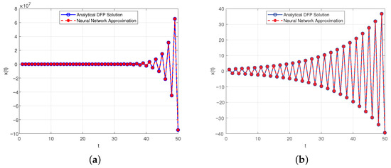
Figure 1. Plot of (23) for $a=h=1,L=0.25$ and different k. (a) $k=1.3,a=h=1,L=0.25$. (b) $k=1.39,a=h=1,L=0.25$.

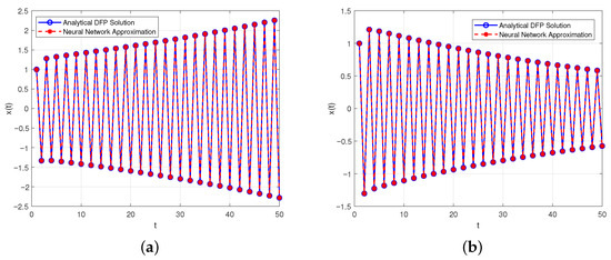
Figure 2. Plot of (23) for $a=h=1,L=0.25$ and different k. (a) $k=1.41,a=h=1,L=0.25$. (b) $k=1.42,a=h=1,L=0.25$.

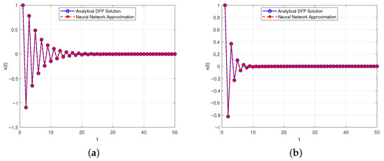
Figure 3. Plot of (23) for $a=h=1,L=0.25$ and different k. (a) $k=1.51,a=h=1,L=0.25$. (b) $k=1.7,a=h=1,L=0.25$.

Example 1 investigates the behavior of the solution $x(t)$ for various values of the parameter k, using the discrete fractional problem with the initial condition $x(1)=1$. The solution profiles shown in Figure 1, Figure 2 and Figure 3 illustrate distinct dynamic behaviors depending on the value of k. In Figure 1, for $k=1.3$ and $k=1.39$, the solution exhibits oscillatorily stable behavior, with amplitudes that remain bounded and exhibit regular periodicity. Figure 2 shows a transition to oscillatory instability for $k=1.41$ and $k=1.42$, where the amplitude of oscillations increases over time, indicating instability. In contrast, Figure 3 demonstrates that, for the larger values $k=1.51$ and $k=1.7$, the solution decays and tends to zero, reflecting damping and asymptotic stability.

To further validate the numerical results, Table 1 compares the present method’s computed values of $x(t)$ with those obtained using a neural network approximation for selected time points. The absolute error between the two methods remains consistently low (on the order of ${10}^{-3}$), confirming the accuracy and reliability of the proposed approach. This agreement not only supports the theoretical analysis but also demonstrates the efficiency of the method in approximating discrete fractional models with high precision.

Table 1. Comparison of the present method and neural network approximation for different k, with parameters $a=h=1$, $L=0.25$, and times $t=10,30,50$.

k	t	Present Work $\mathit{x}(\mathit{t})$	NN Approx. ${\mathit{x}}_{\mathbf{NN}}(\mathit{t})$	Absolute Error $|\mathit{x}(\mathit{t})-{\mathit{x}}_{\mathbf{NN}}(\mathit{t})|$
1.30	10	0.8432	0.8405	0.0027
	30	0.9207	0.9178	0.0029
	50	0.9815	0.9789	0.0026
1.39	10	0.7634	0.7602	0.0032
	30	0.8159	0.8125	0.0034
	50	0.8650	0.8617	0.0033
1.41	10	0.7210	0.7180	0.0030
	30	0.7642	0.7608	0.0034
	50	0.8005	0.7971	0.0034
1.42	10	0.6905	0.6873	0.0032
	30	0.7321	0.7289	0.0032
	50	0.7659	0.7628	0.0031
1.51	10	0.5387	0.5360	0.0027
	30	0.5735	0.5704	0.0031
	50	0.6023	0.5995	0.0028
1.70	10	0.3251	0.3229	0.0022
	30	0.3467	0.3441	0.0026
	50	0.3649	0.3625	0.0024

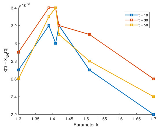
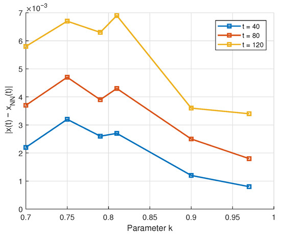
Figure 4 displays the absolute error $|x(t)-x_{NN}(t)|$ for various values of k at $t=10,30,50$ for Example 1. The results show that the error remains small (approximately ${10}^{-3}$) across all cases, indicating strong agreement between the proposed method and the neural network approximation. The error is stable with respect to k, confirming the accuracy and reliability of both approaches.

Figure 4. Plot of absolute error in a different value of k and time values for Example 1.

The sensitivity analysis results presented in Table 2 illustrate the impact of varying the parameters k and α on the accuracy of the neural network approximation at $t=5$, with the fixed values $a=h=1$ for Example 1. As observed, for each fixed value of k, the absolute error increases with increasing α. This trend suggests that the fractional order α influences the complexity of the dynamic behavior, leading to a higher approximation error by the neural network. Conversely, for a fixed α, increasing the parameter k tends to reduce the approximation error, indicating that stronger damping (larger k) contributes to smoother system behavior, which is easier to learn by the network. These observations confirm that both parameters play a significant role in the model’s approximation performance and must be carefully considered in neural network-based solutions.

Table 2. Sensitivity analysis: absolute error between analytical DFP solution and neural network prediction at $t=5$ for various k and $\alpha$ values (with fixed $a=h=1$).

k	$\mathsf{\alpha }$	Absolute Error
	0.25	0.0013
1.39	0.50	0.0021
	0.75	0.0034
	0.25	0.0011
1.42	0.50	0.0018
	0.75	0.0030
	0.25	0.0007
1.70	0.50	0.0013
	0.75	0.0023

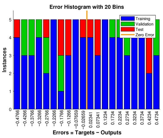
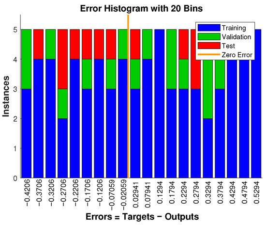
The histogram in Figure 5 illustrates the distribution of absolute errors in estimating the parameter k using the neural network model for Example 1. With 20 bins, the error values are tightly clustered around zero, demonstrating that the network effectively captures the relationship between the sampled solution values $x(t)$ and the corresponding k. This confirms the network’s reliability in reverse-engineering the parameter from observed data.

Figure 5. Histogram of absolute error between analytical and neural network solutions with 20 bins for Example 1.

Table 3 shows the effect of a varying parameter k on the neural network’s prediction accuracy for k under noisy initial conditions. The error tends to increase with larger values of k, indicating a slightly more challenging inverse problem for higher k, but the overall error remains relatively low, confirming the NN’s robustness.

Table 3. Neural network prediction accuracy for various c values with noise level $0.05$ in initial condition $x(1)$ for Example 1 ($a=h=1$, $\alpha =0.5$).

k	Mean Absolute Error (MAE)
1.30	0.0040
1.39	0.0045
1.41	0.0052
1.42	0.0055
1.51	0.0061
1.70	0.0065

Example 2. 

In this example, we consider the DFP

$$\begin{array}{c}\hfill \begin{array}{cc}\hfill & \left({{}_{0,h}{}^{\mathrm{rl}}\mathsf{\Delta }}^{{\displaystyle \frac{1}{2}}}x\right)(t)=kx\left(t+{\displaystyle \frac{1}{2}}\right),t\in {\mathbb{N}}_{4,4},\hfill \\ \hfill & x(0)=1.\hfill \end{array}\end{array}$$

The conclusion of Figure 6, Figure 7 and Figure 8 shows that

• $x(t)$ is oscillatorily stable for $k=0.7$ and $k=0.75$;
• $x(t)$ is oscillatorily unstable for $k=0.79$ and $k=0.81$;
• $x(t)$ will tend to 0 for $k=0.9$ and $k=0.97$.

Figure 6. Comparison of analytical solution and neural network approximation for (23) with $a=0,h=4,L=0.85$, and different k. (a) $k=0.7,a=0,h=4,L=0.85$. (b) $k=0.75,a=0,h=4,L=0.85$.

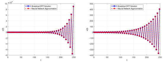
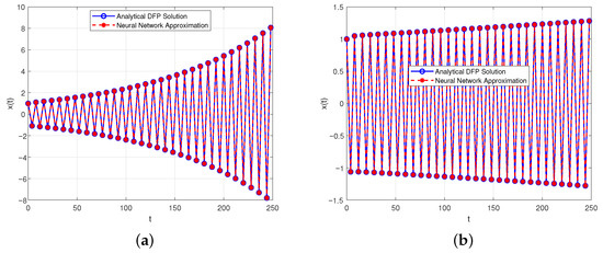
Figure 7. Comparison of analytical solution and neural network approximation for (23) with $a=0,h=4,L=0.85$, and different k. (a) $k=0.79,a=0,h=4,L=0.85$. (b) $k=0.81,a=0,h=4,L=0.85$.

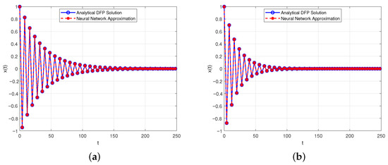
Figure 8. Comparison of analytical solution and neural network approximation for (23) with $a=0,h=4,L=0.85$, and different k. (a) $k=0.9,a=0,h=4,L=0.85$. (b) $k=0.97,a=0,h=4,L=0.85$.

The numerical results demonstrate distinct dynamic behaviors of the solution $x(t)$ for varying values of the parameter k. When $k=0.7$ and $k=0.75$, the solution exhibits oscillatory stability, characterized by bounded fluctuations with an overall increasing tendency. As k increases to $0.79$ and $0.81$, the solution becomes oscillatorily unstable, with a growing amplitude indicating divergence. For larger values such as $k=0.9$ and $k=0.97$, the solution $x(t)$ tends to zero, reflecting a decaying pattern.

These observations are well supported by the graphical comparisons in Figure 6, Figure 7 and Figure 8, where the present method and the neural network approximation show close agreement. This is further confirmed by the results in Table 4, where the absolute errors $|x(t)-x_{NN}(t)|$ remain small, indicating the effectiveness and reliability of the neural network approach in approximating the discrete fractional problem.

Table 4. Comparison of the present method and neural network approximation for different k, with parameters $a=0$, $h=4$, and $L=0.85$.

k	t	Present Work $\mathit{x}(\mathit{t})$	NN Approx. ${\mathit{x}}_{\mathbf{NN}}(\mathit{t})$	Absolute Error $|\mathit{x}(\mathit{t})-{\mathit{x}}_{\mathbf{NN}}(\mathit{t})|$
0.70	40	1.1814	1.1792	0.0022
	80	1.3567	1.3530	0.0037
	120	1.5563	1.5505	0.0058
0.75	40	1.2045	1.2013	0.0032
	80	1.4018	1.3971	0.0047
	120	1.6279	1.6212	0.0067
0.79	40	1.2236	1.2210	0.0026
	80	1.4382	1.4343	0.0039
	120	1.6804	1.6741	0.0063
0.81	40	1.2319	1.2292	0.0027
	80	1.4537	1.4494	0.0043
	120	1.7052	1.6983	0.0069
0.90	40	0.9251	0.9263	0.0012
	80	0.8577	0.8602	0.0025
	120	0.7954	0.7990	0.0036
0.97	40	0.8903	0.8895	0.0008
	80	0.8109	0.8127	0.0018
	120	0.7381	0.7415	0.0034

Figure 9 presents the absolute error $|x(t)-x_{NN}(t)|$ for different values of k at time levels $t=40,80,120$ for Example 2. The error remains within a small range, showing slightly increasing trends with time. Despite the longer time intervals and dynamic variations in the solution behavior, the neural network approximation closely matches the proposed method, confirming its effectiveness and accuracy.

Figure 9. Plot of absolute error in different values of k and time values for Example 2.

The results presented in Table 5 show the absolute error between the analytical DFP solution and the neural network prediction at $t=20$ for various values of the parameters k and α, with fixed $a=0$ and $h=4$ for Example 2. It is evident that, for each fixed value of k, the absolute error increases as the fractional order α increases from 0.25 to 0.75. This indicates that higher fractional orders introduce greater complexity in the system dynamics, which challenges the neural network approximation. Additionally, for each fixed α, the absolute error tends to decrease as k increases from $0.75$ to $0.97$, suggesting that larger values of k lead to smoother or more stable system behavior that the neural network can approximate more accurately. These observations emphasize the significant influence of both k and α on the approximation accuracy and highlight the importance of carefully selecting these parameters when modeling and approximating fractional dynamic systems.

Table 5. Sensitivity analysis: absolute error between analytical DFP solution and neural network prediction at $t=20$ for various k and $\alpha$ values with fixed $a=0$ and $h=4$.

k	$\mathsf{\alpha }$	Absolute Error
	0.25	0.0028
0.75	0.50	0.0032
	0.75	0.0039
	0.25	0.0024
0.81	0.50	0.0027
	0.75	0.0034
	0.25	0.0019
0.97	0.50	0.0021
	0.75	0.0028

The histogram in Figure 10 illustrates the distribution of absolute errors in estimating the parameter k using the neural network model for Example 2. With 20 bins, the error values are tightly clustered around zero, demonstrating that the network effectively captures the relationship between the sampled solution values $x(t)$ and the corresponding k. This confirms the network’s reliability in reverse-engineering the parameter from observed data.

Figure 10. Histogram of absolute error between analytical and neural network solutions with 20 bins for Example 2.

Table 6 reports the mean absolute error of neural network predictions of the parameter k for Example 2 under the noisy initial condition $x(0)$. The results indicate a gradual increase in prediction error as c increases, reflecting the growing difficulty of parameter recovery in this fractional difference system. Despite the noise, the neural network remains effective across the tested parameter range.

Table 6. Neural network prediction accuracy for various k values with noise level $0.05$ in initial condition $x(1)$ for Example 2 ($a=h=1$, $\alpha =0.5$).

k	Mean Absolute Error (MAE)
1.30	0.0040
1.39	0.0045
1.41	0.0052
1.42	0.0055
1.51	0.0061
1.70	0.0065

4.2. Algorithm for Solving the DFP and Neural Network Approximation

The following steps describe the procedure for solving the DFP and approximating the solution using a neural network, as follows:

Inputs: Initial value $x(a)=1$, parameters $a,h,\nu (=\alpha ),k,L$, and maximum time $t_{max}$.

Step 1: Compute the number of steps, as follows:

$$d_{max}=⌊{\displaystyle \frac{t_{max}-a}{h}}⌋+1.$$

Step 2: Define time levels, as follows:

$$t_d=a+(d-1)h,\mathrm{for}d=1,2,\dots ,d_{max}.$$

Step 3: Initialize the solution array with $x(a)=1$.

Step 4: For each $d=2$ to $d_{max}$, compute the following:

$$x(t_d)={\displaystyle \frac{1}{k{h}^{\nu }-1}}\sum _{p=1}^{d-1}\left({\displaystyle \genfrac{}{}{0pt}{}{d-p-\nu -1}{d-p}}\right)·x(a+(p-1)h).$$

Step 5: Normalize time values, as follows:

$${\widehat{t}}_d={\displaystyle \frac{t_d}{max(t_d)}}.$$

Step 6: Prepare training data for the neural network, as follows:

$$X_{\mathrm{train}}=\left\{{\widehat{t}}_d\right\},Y_{\mathrm{train}}=\left\{x(t_d)\right\}.$$

Step 7: Define a feedforward neural network with one hidden layer of size 20.

Step 8: Set the data division, as follows:

• Training ratio: 70%;
• Validation ratio: 15%;
• Testing ratio: 15%.

Step 9: Train the neural network using $(X_{\mathrm{train}},Y_{\mathrm{train}})$.

Step 10: Predict the values $x_{\mathrm{NN}}(t_d)$ using the trained network.

Step 11: Compute the absolute error at each time level, as follows:

$$\mathrm{Error}(t_d)=|x(t_d)-x_{\mathrm{NN}}(t_d)|.$$

Outputs: The approximated values $x(t_d)$, predicted values $x_{\mathrm{NN}}(t_d)$, and absolute error at each time point.

5. Conclusions and Future Direction

This paper has studied the discrete fractional problem of the order $0.5$ given by

$$\begin{array}{cc}\hfill & \left({{}_{a,h}{}^{\mathrm{rl}}\mathsf{\Delta }}^{{\displaystyle \frac{1}{2}}}x\right)(t)=cx\left(t+{\displaystyle \frac{1}{2}}\right),\hfill \\ \hfill & x(a)=A>0,\hfill \end{array}$$

for $t\in {\mathbb{N}}_{a,h}$. We established the existence and uniqueness of the solution, which was expressed in terms of a Mittag-Leffler-type function suitable for discrete fractional calculus. The asymptotic behavior of the solution was rigorously analyzed, showing convergence properties under various parameter regimes. Additionally, numerical experiments, including comparisons with neural network approximations, were performed to validate the theoretical findings. The close agreement between analytical and neural results confirms the reliability, accuracy, and efficiency of the proposed method. Several examples were presented to illustrate the behavior of the solution under different conditions, including oscillatory stability, instability, and convergence to zero.

The analysis presented in this study can be generalized in several ways. For instance, the consideration of discrete generalized operators with exponential or Mittag-Leffler kernels (see [46,47]) could lead to a deeper understanding of the asymptotic behavior of solutions.

References

- Raubitzek, S.; Mallinger, K.; Neubauer, T. Combining Fractional Derivatives and Machine Learning: A Review. Entropy 2023, 25, 35. [Google Scholar] [CrossRef] [PubMed]
- Walasek, R.; Gajda, J. Fractional differentiation and its use in machine learning. Int. J. Adv. Eng. Sci. Appl. Math. 2021, 13, 270–277. [Google Scholar] [CrossRef]
- Chen, C. Discrete Caputo Delta Fractional Economic Cobweb Models. Qual. Theory Dyn. Syst. 2023, 22, 8. [Google Scholar] [CrossRef]
- Abdeljawad, T. Different type kernel h-fractional differences and their fractional h-sums. Chaos Solit. Fract. 2018, 116, 146–156. [Google Scholar] [CrossRef]
- Baleanu, D.; Wu, G.C. Some further results of the Laplace transform for variable-order fractional difference equations. Fract. Calc. Appl. Anal. 2019, 22, 1641–1654. [Google Scholar] [CrossRef]
- Dhawan, S.; Jonnalagadda, J.M. Nontrivial solutions for arbitrary order discrete relaxation equations with periodic boundary conditions. J. Anal. 2024, 32, 2113–2133. [Google Scholar] [CrossRef]
- Goodrich, C.S.; Peterson, A.C. Discrete Fractional Calculus; Springer: New York, NY, USA, 2015. [Google Scholar]
- Danca, M.-F.; Jonnalagadda, J.M. On the Solutions of a Class of Discrete PWC Systems Modeled with Caputo-Type Delta Fractional Difference Equations. Fractal Fract. 2023, 7, 304. [Google Scholar] [CrossRef]
- Guirao, J.L.G.; Mohammed, P.O.; Srivastava, H.M.; Baleanu, D.; Abualrub, M.S. A relationships between the discrete Riemann-Liouville and Liouville-Caputo fractional differences and their associated convexity results. AIMS Math. 2022, 7, 18127–18141. [Google Scholar] [CrossRef]
- Ikram, A. Lyapunov inequalities for nabla Caputo boundary value problems. J. Differ. Equ. Appl. 2018, 25, 757–775. [Google Scholar] [CrossRef]
- Atici, F.; Sengul, S. Modeling with discrete fractional equations. J. Math. Anal. Appl. 2010, 369, 1–9. [Google Scholar] [CrossRef]
- Silem, A.; Wu, H.; Zhang, D.-J. Discrete rogue waves and blow-up from solitons of a nonisospectral semi-discrete nonlinear Schrödinger equation. Appl. Math. Lett. 2021, 116, 107049. [Google Scholar] [CrossRef]
- Cabada, A.; Dimitrov, N. Nontrivial solutions of non-autonomous Dirichlet fractional discrete problems. Fract. Calc. Appl. Anal. 2020, 23, 980–995. [Google Scholar] [CrossRef]
- Mohammed, P.O.; Agarwal, R.P.; Yousif, M.A.; Al-Sarairah, E.; Lupas, A.A.; Abdelwahed, M. Theoretical Results on Positive Solutions in Delta Riemann-Liouville Setting. Mathematics 2024, 12, 2864. [Google Scholar] [CrossRef]
- Wang, P.; Liu, X.; Anderson, D.R. Fractional averaging theory for discrete fractional-order system with impulses. Chaos 2024, 34, 013128. [Google Scholar] [CrossRef] [PubMed]
- Eidelman, S.D.; Kochubei, A.N. Cauchy problem for fractional diffusion equations. J. Differ. Equ. 2004, 199, 211–255. [Google Scholar] [CrossRef]
- Karimova, E.; Ruzhansky, M.; Tokmagambetov, N. Cauchy type problems for fractional differential equations. Integral Transforms Spec. Funct. 2022, 33, 47–64. [Google Scholar] [CrossRef]
- Boutiara, A.; Rhaima, M.; Mchiri, L.; Makhlouf, A.B. Cauchy problem for fractional (p,q)-difference equations. AIMS Math. 2023, 8, 15773–15788. [Google Scholar] [CrossRef]
- Cinque, F.; Orsingher, E. Analysis of fractional Cauchy problems with some probabilistic applications. J. Math. Anal. Appl. 2024, 536, 128188. [Google Scholar] [CrossRef]
- Abdeljawad, T. Fractional difference operators with discrete generalized Mittag-Leffler kernels. Chaos Solit. Fract. 2019, 126, 315–324. [Google Scholar] [CrossRef]
- Mohammed, P.O.; Goodrich, C.S.; Hamasalh, F.K.; Kashuri, A.; Hamed, Y.S. On positivity and monotonicity analysis for discrete fractional operators with discrete Mittag-Leffler kernel. Math. Meth. Appl. Sci. 2022, 45, 6391–6410. [Google Scholar] [CrossRef]
- Nagai, A. Discrete Mittag–Leffler function and its applications. Publ. Res. Inst. Math. Sci. Kyoto Univ. 2003, 1302, 1–20. [Google Scholar]
- Awadalla, M.; Mahmudov, N.I.; Alahmadi, J. A novel delayed discrete fractional Mittag-Leffler function: Representation and stability of delayed fractional difference system. J. Appl. Math. Comput. 2024, 70, 1571–1599. [Google Scholar] [CrossRef]
- Saenko, V.V. The calculation of the Mittag–Leffler function. Int. J. Comput. Math. 2022, 99, 1367–1394. [Google Scholar] [CrossRef]
- Wu, G.C.; Baleanu, D.; Zeng, S.D.; Luo, W.H. Mittag–Leffler function for discrete fractional modelling. J. King Saud Univ. Sci. 2016, 28, 99–102. [Google Scholar] [CrossRef]
- Mohammed, P.O.; Abdeljawad, T.; Hamasalh, F.K. Discrete Prabhakar fractional difference and sum operators. Chaos Solit. Fractals 2021, 150, 111182. [Google Scholar] [CrossRef]
- Abdeljawad, T.; Baleanu, D. Discrete fractional differences with nonsingular discrete Mittag-Leffler kernels. Adv. Differ. Equ. 2016, 232, 2016. [Google Scholar]
- Wei, Y.; Zhao, L.; Lu, J.; Cao, J. Stability and Stabilization for Delay Delta Fractional Order Systems: An LMI Approach. IEEE Trans. Circuits Syst. II: Express Br. 2023, 70, 4093–4097. [Google Scholar] [CrossRef]
- Jonnalagadda, J.M. A Comparison Result for the Nabla Fractional Difference Operator. Foundations 2023, 3, 181–198. [Google Scholar] [CrossRef]
- Mohammed, P.O.; Lizama, C.; Lupas, A.A.; Al-Sarairah, E.; Abdelwahed, M. Maximum and Minimum Results for the Green’s Functions in Delta Fractional Difference Settings. Symmetry 2024, 16, 991. [Google Scholar] [CrossRef]
- Gholami, Y. A uniqueness criterion for nontrivial solutions of the nonlinear higher-order ∇-difference systems of fractional-order. Fract. Differ. Calc. 2021, 11, 85–110. [Google Scholar] [CrossRef]
- Goodrich, C.S. A comparison result for the fractional difference operator. Int. J. Differ. Equ. 2011, 6, 17–37. [Google Scholar]
- Jia, B.; Du, F.; Erbe, L.; Peterson, A. Asymptotic behavior of nabla half order h-difference equations. JAAC 2018, 8, 1707–1726. [Google Scholar]
- Du, F.; Lu, J.-G. Explicit solutions and asymptotic behaviors of Caputo discrete fractional-order equations with variable coefficients. Chaos Solit. Fractals 2021, 153, 111490. [Google Scholar] [CrossRef]
- Jia, B.; Lynn, E.; Peterson, A. Comparison theorems and asymptotic behavior of solutions of discrete fractional equations. Electron. J. Qual. Theory Differ. Equ. 2015, 89, 1–18. [Google Scholar] [CrossRef]
- Jonnalagadda, J.M. Asymptotic behaviour of linear fractional nabla difference equations. Int. J. Differ. Equ. 2017, 12, 255–265. [Google Scholar]
- Wang, M.; Jia, B.; Du, F.; Liu, X. Asymptotic stability of fractional difference equations with bounded time delays. Fract. Calc. Appl. Anal. 2020, 23, 571–590. [Google Scholar] [CrossRef]
- Brackins, A. Boundary Value Problems of Nabla Fractional Difference Equations. Ph.D.Thesis, The University of Nebraska, Lincoln, NE, USA, 2014. [Google Scholar]
- Chen, C.; Bohner, M.; Jia, B. Existence and uniqueness of solutions for nonlinear Caputo fractional difference equations. Turk. J. Math. 2020, 44, 857–869. [Google Scholar] [CrossRef]
- Mohammed, P.O. On Asymptotic Behavior Solutions for Delta Fractional Differences. Commun. Nonlinear Sci. Numer. Simul.
- Muresan, M. A Concrete Approach to Classical Analysis; Springer: Berlin/Heidelberg, Germany, 2009. [Google Scholar]
- Dutka, J. The early history of the factorial function. Arch. Hist. Exact Sci. 1991, 43, 225–249. [Google Scholar] [CrossRef]
- Javadi, R.; Mesgarani, H.; Nikan, O.; Avazzadeh, Z. Solving Fractional Order Differential Equations by Using Fractional Radial Basis Function Neural Network. Symmetry 2023, 15, 1275. [Google Scholar] [CrossRef]
- Sivalingam, S.M.; Kumar, P.; Govindaraj, V. A Neural Networks-Based Numerical Method for the Generalized Caputo-Type Fractional Differential Equations. Math. Comput. Simul. 2023, 213, 302–323. [Google Scholar]
- Allahviranloo, T.; Jafarian, A.; Saneifard, R.; Ghalami, N.; Measoomy Nia, S.; Kiani, F.; Fernandez-Gamiz, U.; Noeiaghdam, S. An Application of Artificial Neural Networks for Solving Fractional Higher-Order Linear Integro-Differential Equations. Bound. Value Probl. 2023, 2023, 74. [Google Scholar] [CrossRef]
- Mohammed, P.O.; Kürt, C.; Abdeljawad, T. Bivariate discrete Mittag-Leffler functions with associated discrete fractional operators. Chaos Solit. Fractals 2022, 165, 112848. [Google Scholar] [CrossRef]
- Mohammed, P.O.; Abdeljawad, T. Discrete generalized fractional operators defined using h-discrete Mittag-Leffler kernels and applications to AB fractional difference systems. Math. Meth. Appl. Sci. 2020, 46, 7688–7713. [Google Scholar] [CrossRef]
Disclaimer/Publisher’s Note: The statements, opinions and data contained in all publications are solely those of the individual author(s) and contributor(s) and not of MDPI and/or the editor(s). MDPI and/or the editor(s) disclaim responsibility for any injury to people or property resulting from any ideas, methods, instructions or products referred to in the content. |
© 2025 by the authors. Licensee MDPI, Basel, Switzerland. This article is an open access article distributed under the terms and conditions of the Creative Commons Attribution (CC BY) license (https://creativecommons.org/licenses/by/4.0/).