Abstract
Eigenvalue problems play a fundamental role in many scientific and engineering disciplines, including structural mechanics, quantum physics, and control theory. In this paper, we propose a fast and stable fractional-order parallel algorithm for solving eigenvalue problems. The method is implemented within a parallel computing framework, allowing simultaneous computations across multiple processors to improve both efficiency and reliability. A theoretical convergence analysis shows that the scheme achieves a local convergence order of , where denotes the Caputo fractional order prescribing the memory depth of the derivative term. Comparative evaluations based on memory utilization, residual error, CPU time, and iteration count demonstrate that the proposed parallel scheme outperforms existing methods in our test cases, exhibiting faster convergence and greater efficiency. These results highlight the method’s robustness and scalability for large-scale eigenvalue computations.
1. Introduction
Eigenvalue computation is a fundamental topic in mathematics and science, with applications in structural mechanics; vibration analysis [1,2,3]; and, more recently, in machine learning, signal processing, quantum physics, and stability analysis [4]. Efficient numerical methods are essential for handling large-scale problems in these fields. Analytical approaches based on solving characteristic polynomials are inherently limited. In most eigenvalue problems, the characteristic equation is a polynomial of degree five or higher. The Abel–Ruffini impossibility theorem [5] states that general polynomials of degree five or higher cannot be solved exactly by radicals, making closed-form analytical factorization impossible. Therefore, numerical methods must be used to compute eigenvalues accurately. Existing numerical techniques, while effective in many cases, can face limitations in computational efficiency, stability, and convergence speed, particularly for large-scale problems or when dealing with clustered or ill-conditioned eigenvalue distributions. These considerations motivate the development of fractional-order parallel algorithms, which leverage fractional calculus and parallel computing to improve accuracy, accelerate convergence, and reduce computational costs.
Classical iterative methods, such as the Power Method and Inverse Iteration, compute one eigenvalue at a time but suffer from several drawbacks:
- Local convergence depends on an appropriate initial guess.
- Performance deteriorates when eigenvalues are closely spaced.
- Convergence slows or stalls when the derivative of the iterative function approaches zero.
- Sequential computation is inefficient for large-scale problems.
On the other hand, parallel algorithms, including both integer- and fractional-order approaches, offer a promising alternative by computing multiple eigenvalues simultaneously while optimizing memory and processing resources. Several parallel techniques have been developed to enhance eigenvalue computation efficiency. The Jacobi and Divide-and-Conquer methods are widely used for symmetric eigenvalue problems. The Divide-and-Conquer algorithm () [6] recursively decomposes the problem into smaller subproblems, facilitating efficient computation on modern multi-core systems, while the Jacobi method [7] applies concurrent rotations for matrix diagonalization. Additionally, QR and Generalized Shur Decomposition Method () algorithms [8] have been parallelized using block matrix operations to accelerate convergence [9,10]. Important advantages of parallel and fractional-order approaches include the following:
- Fractional-order methods incorporate historical information, enhancing convergence speed and accuracy.
- Modern high-performance architectures reduce computation time.
- Improved numerical stability for complex eigenvalue problems.
- Higher precision without sacrificing efficiency.
- Faster convergence with fewer iterations, reducing computational costs.
This evolution in numerical methods continues to drive progress in large-scale eigenvalue computations, enabling more efficient solutions across scientific and engineering disciplines. For large-scale eigenvalue problems, Krylov subspace-based algorithms such as the Parallel Lanczos [11] and Arnoldi methods [12] provide effective solutions by computing multiple eigenvalues within high-performance computing environments. More recent advancements, including Ehrlich techniques [13] and Weierstrass parallel methods [14], distribute the computational load across multiple processors to enhance efficiency. However, when applied to non-Hermitian or large sparse matrices, these approaches often face scaling limitations, numerical instability, and increased memory demands.
This study aims to develop a high-order, fractional Caputo-based parallel scheme that significantly enhances computational efficiency and accuracy. The proposed fractional-order parallel algorithm achieves an optimal convergence order, outperforming conventional techniques in both precision and performance. By leveraging the memory-preserving properties of fractional calculus, the method improves numerical stability while reducing computational overhead. Unlike traditional parallel schemes, the approach minimizes the number of required iterations, optimizing the use of computational resources. In real-world applications, many stability issues are fundamentally linked to eigenvalue problems. For example, in car dynamics, the linearized eigenvalues of the suspension-steering system determine pitch and roll stability, as well as ride comfort; a positive real part indicates a loss of control under disturbances. In aeroelasticity, aircraft wing flutter is diagnosed by monitoring the eigenvalues of the coupled structural–aerodynamic model, with flutter onset identified by the crossing of the imaginary axis by a complex conjugate eigenvalue pair. Since virtually all engineering stability analyses require eigenvalues to be computed with high precision, efficient iterative techniques for nonlinear eigenvalue problems are essential. The proposed scheme is validated on eigenvalue problems related to car stability and aircraft wing flutter, demonstrating its practical relevance. In addition, we introduce the fundamental concepts of fractional calculus that are critical for constructing and analyzing the parallel schemes. In particular, the Caputo derivative is one of the few fractional derivatives that satisfy the condition [15]. The Caputo derivative of order incorporates a weighted history integral that smooths oscillations in the iterative map and prevents the derivative term from vanishing when the ordinary first derivative approaches zero. This feature helps reduce divergence around flat regions or multiple roots, enhancing the robustness of the iterative process.
Definition 1
(Caputo fractional derivative). Let
where , and is the integer part of . The Caputo fractional derivative [16,17] of order is defined as
Here, denotes the Gamma function, given by
Remark 1.
The notation indicates that f is m-times continuously differentiable on the closed interval . This regularity is necessary to ensure that the m-th derivative appearing in (2) exists and is continuous.
The Caputo derivative is adopted in this study because it offers several practical advantages over other fractional derivative definitions:
- The Caputo derivative of a constant is zero, preserving the classical interpretation of steady-state solutions. In contrast, the Grünwald–Letnikov (GL) derivative yields nonzero values, complicating model interpretation.
- Unlike the GL definition, the Caputo derivative requires only integer-order initial conditions. This allows empirically observed values to be directly incorporated without introducing additional fractional history terms.
- Caputo operators improve the stability and convergence of higher-order iterative solvers by ensuring more consistent kernel behavior. Due to these advantages, the Caputo derivative is almost universally preferred in dynamical models and is particularly well suited for parallel fractional framework schemes.
The Taylor series theorem (Appendix A.1) provides a local approximation of a function near its root and serves as the foundation for iterative methods used to solve nonlinear equations. Expanding a function into its Taylor series, including higher-order terms, leads to more accurate and efficient iterative schemes. This approach underpins both function linearization and acceleration towards the root. Each of these classical methods forms the basic foundation for our novel family of fractional schemes. After developing the fractional versions, we incorporate them as correction steps within a parallel architecture capable of approximating all eigenvalues simultaneously in a single iteration step.
Using a Caputo-type fractional variant of Newton’s method (), Candelario et al. [18] introduced the following iteration scheme:
where . For any , the order of convergence of this method is , with the error given by the following:
where and , with
Shams et al. [19] proposed a one-step fractional iterative method with order , given by
which satisfies the error relation
where .
Ali et al. [20] later proposed a modified scheme of the following convergence order:
where
for , satisfying the following error equation:
In [21], a two-step fractional Newton-type method with convergence order was introduced:
where
satisfying the error relation
where , , and , The propagation of the local error from one iteration to the next is described by Equations (5), (7), (9) and (11). A complete derivation is not included here, as it follows the classical fractional Taylor expansion and perturbation arguments provided in [18,19,20,21]. Substituting the series expansion of f about the exact root into the fractional correction step produces a power-law term in , indicating a convergence order that explicitly depends on the fractional parameter.
The rest of this manuscript is structured as follows. Section 2 introduces and analyzes the proposed fractional-order scheme. Section 3 examines the region of percentage convergence using basins of attraction. Section 4 explores engineering applications, evaluating the proposed method in terms of efficiency, stability, and consistency against existing methods. Finally, Section 5 presents conclusions and potential future research directions.
2. Development and Analysis of the Caputo-Type Fractional Schemes
Classical numerical iterative schemes suffer from several drawbacks, such as the omission of memory effects, divergence of higher-order derivatives, slow convergence, and the limitation to computing only real roots in almost all situations. These issues reduce the precision of models for complex systems with long-range dependencies. Fractional-order approaches address these issues by leveraging historical data, enhancing stability, and simulating nonlocal processes. Therefore, they are more suitable for procedures that require higher model accuracy. The memory- and nonlocal-effect approach can be effectively modeled using Caputo fractional derivatives, providing a more realistic simulation of dynamic systems. The weight function dynamically modifies the scheme based on the ratio of function values between current and previous iterations. This dynamic adjustment aids in stabilizing and accelerating convergence, particularly under conditions where classical methods may struggle. To improve the convergence order of the existing technique (10), we propose a modified version that incorporates the weight function into the second step of (10). The updated formulation () is given by the following:
where
and the weight function , which depends on the parameter
is specifically designed to guarantee fourth-order convergence, as demonstrated in Theorem 1.
2.1. Convergence Analysis
Convergence analysis is essential for assessing the reliability and efficiency of numerical methods used to solve nonlinear equations. It establishes the conditions under which an iterative approach converges to the desired solution. The local convergence properties of the proposed method are examined in Theorem 1.
Theorem 1.
Let be a continuous function, where is of order m, for any positive integer m and in the open interval , and let denote the exact root of .
If the initial value is sufficiently close to , and the function satisfies
then the iterative scheme
has a convergence order of at least , with the associated error given by
where
and
is defined in Appendix A.2.
Proof.
Let be a root of , and define , , and . We assume that the function is smooth in a neighborhood of the root , with no discontinuities or singularities in the region under consideration. In particular, should be continuously differentiable up to the required order, and the fractional derivative should also be free from singularities in this region. Expanding and using their Taylor series around and noting that , we obtain.
Taking fractional derivative of (15) yields
Thus,
Expanding around using a Taylor series, we obtain
Expanding as a Taylor series, we obtain
where Thus,
Therefore,
This simplifies to
The coefficients are given by
The expression for is provided in Appendix A.2. By choosing and , we conclude
Thus, the theorem is proven. □
2.2. Some Special Cases of the Proposed Fractional Schemes Are Considered
Weight functions play a crucial role in iterative methods for solving nonlinear equations by enhancing convergence speed and stability. They help regulate the influence of previous iterations, improving accuracy while reducing computational costs. A well-designed weight function adaptively balances efficiency and robustness, leading to more reliable numerical solutions. Building on the conditions established in Theorem 1, we introduce several distinct weight function formulations to optimize iterative algorithms, as outlined below.
Fractional Scheme : By selecting the weight function
which satisfies the conditions of Theorem 1, we derive the following fractional scheme:
where . Here, is defined as
The associated error equation is given by
Fractional Scheme : By selecting the weight function
which satisfies the conditions of Theorem 1, we derive the following fractional scheme:
Here, is defined as
The associated error equation is given by
Fractional Scheme : By selecting the weight function
which satisfies the conditions of Theorem 1, we derive the following fractional scheme:
where . Here, is defined as
The associated error equation is given by
In the following section, we demonstrate how transforming single-eigenvalue methods into parallel fractional approaches enhances computational efficiency by solving for all eigenvalues simultaneously, thereby reducing the number of iterations. This method improves stability and convergence by leveraging interdependencies between eigenvalues, effectively minimizing errors. Moreover, fractional parallel techniques offer a more precise and reliable solution for eigenvalue problems involving clustered or multiple eigenvalues.
3. Parallel Computing Scheme Construction and Theoretical Convergence
Among parallel numerical schemes, the Weierstrass–Durand–Kerner approach [22] is particularly appealing from a computational perspective. In this technique, each eigenvalue contributes to the approximation of the others, allowing for efficient parallel implementation. Its structure allows simultaneous updates, making it ideal for parallel computing architectures. This method is defined a
where
represents Weierstrass’s correction. The method in (37) exhibits local quadratic convergence.
Nedzibov et al. [23] proposed a modified Weierstrass method:
This is also known as the inverse Weierstrass method, which retains quadratic convergence. The inverse parallel scheme in (39) also demonstrates local quadratic convergence.
In 1977, Ehrlich [24] introduced a third-order simultaneous iterative method defined as
Zhang et al. [25] proposed an iterative method with convergence order five, given by
Here, the term is defined as
Using as a correction in (40), Petkovic et al. [26] improved the convergence order from three to six, resulting in the following scheme:
Here, is given by
where
This technique is also applied in biomedical engineering to solve nonlinear equations, enabling the analysis of various problems and treatment methodologies. Here, we consider the following iterative scheme [27] for finding simple roots of nonlinear equations.
The method proposed in [28] has been shown to achieve higher accuracy, faster convergence, robustness, and improved computational efficiency compared to conventional single root-finding techniques. The iterative scheme is defined as
where
The scheme has a convergence order of 6 and satisfies the following local error relation:
where
and
By replacing with in (38) and applying Weierstrass’s correction in (43), we derive a new parallel scheme for simultaneously computing all eigenvalues:
Here, the intermediate values are defined as
Additionally, the correction terms for different schemes are given by
Fractional-order methods are employed as correction terms within the parallel architecture to enhance its reliability. These schemes improve both the convergence and stability of the parallel approach. In particular, when roots are closely spaced, fractional derivatives help prevent the divergence that often occurs in traditional parallel structures. By incorporating these techniques, the parallel root-finding scheme becomes more efficient and yields more accurate and stable solutions to eigenvalue problems. The resulting parallel schemes are denoted as . The methods can be rewritten a
where
For multiple roots, the method is extended as
where
The following theorem defines the local order of convergence for the inverse fractional scheme.
Theorem 2.
Let be simple roots of a nonlinear equation and assume that the initial distinct approximations are sufficiently close to the exact roots. Then, the – method achieves a convergence order of .
Proof.
Let , and represent the errors in , , and , respectively. From the first step of the – method, we obtain
Rewriting in terms of error terms, we obtain
which simplifies to
From the Taylor series expansion, we approximate
Since , we obtain
Thus, we derive
For the second step,
Rewriting in terms of the error terms, we obtain
Since
we obtain the following using the error propagation assumption.
Assuming , we obtain
Since , we conclude
This completes the proof. □
4. Computational Efficiency and Numerical Results
Computational efficiency in parallel iterative methods is crucial for solving complex problems while minimizing computational costs. Analyzing efficiency allows us to identify numerical schemes that require fewer arithmetic operations while maintaining accuracy, stability, and consistency in solving eigenvalue problems. Efficient algorithms reduce execution time, making them particularly well suited for large-scale simulations and real-time applications. Comparing computational performance helps in selecting methods that maximize efficiency without compromising precision. Optimized numerical schemes are especially valuable in high-performance computing and engineering contexts, where computational resources are limited and reliability is essential. The computational efficiency of a parallel scheme is an important metric for evaluating how effectively it solves a problem, especially in terms of resource usage such as time, memory and the number of operations. To quantify this efficiency, we use the expression
where E denotes the computing efficiency, r is the convergence order of the fractional-order parallel scheme, and represents the total computational cost of the algorithm. The cost is computed as the weighted sum of all computational operations performed at each step [29]:
Here, we have the following:
- represents the number of additions and subtractions.
- is the number of multiplications.
- denotes the number of divisions required for a polynomial of degree n.
The constants , , and are weights that reflect the relative computational cost of each operation type (division, multiplication, and addition) in each iteration. These weights are empirically determined based on the performance characteristics of the computing platform or hardware in use. These considerations are critical for analyzing large-scale systems and improving the overall accuracy and robustness of solutions. Based on the data in Table 1, the percentage computational efficiency (65) is calculated using
which can be used to assess the performance of newly developed parallel schemes in comparison to existing methods in the literature. In terms of consistency, stability, and percentage computational efficiency, the following numerical schemes—classified by their convergence order—are analyzed:

Table 1.
Numerical results of parallel schemes for solving eigenvalue problems.
- Perkovic et al.’s method () [30] is as follows:where
- Wang–Wu’s parallel scheme () [31] is as follows:
- The Farmer–Loizou-like technique () [32] is combined with Newton’s method at the first step:where
Table 2 and Figure 1 present the computing efficiency percentage of the newly developed methodology compared to the previous approach. The results indicate that the proposed method requires fewer basic mathematical operations per iteration and consumes less memory compared to other existing schemes.
Table 2.
Percentage computational efficiency and memory utilization of parallel schemes.

Figure 1.
Computational efficiency comparison of the , , , and - parallel architectures.
Using the information from Table 2 and the corresponding stopping criterion
the effectiveness, stability, and consistency of the newly developed method, in relation to existing strategies for biomedical engineering applications, are analyzed in the following sections. Here, represents the absolute error or the norm-2 measure of error.
The eigenvalue problems chosen for numerical experiments, such as automotive suspension systems and aviation wing models, are chosen because of their real-world engineering importance and inherent mathematical complexity. They provide higher-degree characteristic polynomials, making them ideal for validating numerical eigenvalue techniques. Eigenvalues have a direct impact on natural frequency and damping ratio in automobile systems, which in turn affect ride stability and comfort. Eigenvalue-based flutter analysis is used in aircraft constructions to predict critical speeds and the structural reaction to aerodynamic loads. Their decision is based on practical applicability, computational complexity, and potential generalizability to other advanced engineering systems, making them suitable for numerical experimentation. To ensure clarity and reproducibility, Algorithm 1 and flowchart Figure 2 present a step-by-step procedure for approximating all eigenvalues simultaneously.
| Algorithm 1: Fractional order parallel scheme for finding all eigenvalues simultaneously. |
|
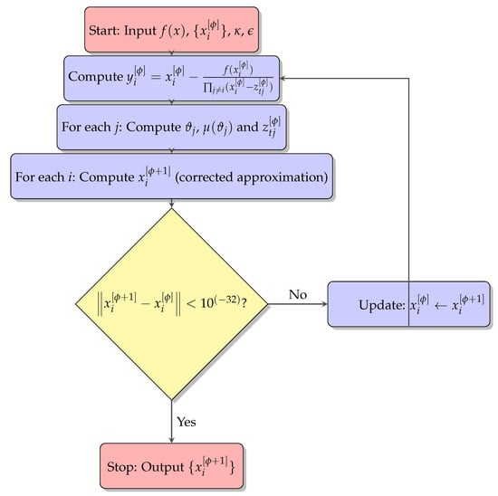
Figure 2.
Flowchart of the fractional-order parallel schemes for simultaneously finding all eigenvalues.
4.1. Mechanical Engineering Model for Automotive Suspension [33]
To solve a mechanical system with multiple degrees of freedom (MDOF), consider the example of an automotive suspension system. In such systems, the governing equations of motion can be formulated and analyzed using eigenvalue techniques. The objective is to derive the governing equations, obtain the characteristic polynomial, and determine the eigenvalues of a polynomial of degree greater than six.
Consider a simplified model of an automotive suspension system, as illustrated in Figure 3a,b [34]. The system consists of a car body (m) mounted on four springs (stiffness k) and dampers (damping coefficient c). While the analysis will be extended to a higher-degree-of-freedom (DOF) system, the initial representation can be approximated as a two-degree-of-freedom (2DOF) system.
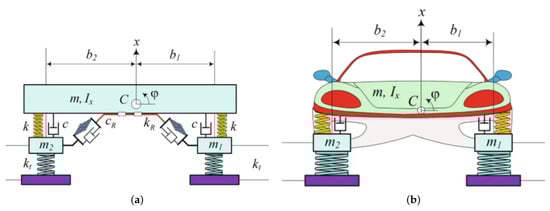
Figure 3.
(a,b) Stability analysis of the car and its corresponding suspension system. (a) Car suspension system; (b) detailed view of the car suspension system.
4.1.1. Model Assumptions
- The system is linear.
- The suspension consists of multiple springs and dampers, each representing a distinct suspension component.
4.1.2. Governing Equations
The equations of motion for a system with multiple degrees of freedom can be expressed in matrix form as follows:
where the following is the case:
- is the displacement vector of the masses.
- is the mass matrix.
- is the damping matrix.
- is the stiffness matrix.
- is the external force vector.
For a system with n degrees of freedom, the mass (), damping (), and stiffness () matrices take the following forms:
Assume a harmonic solution of the form given in Equation (72):
The eigenvalues of the system are obtained by setting , leading to the following characteristic equation:
For a system with n degrees of freedom, the characteristic polynomial of degree n is given by
The above model can be solved for specific cases, such as and degrees of freedom.
4.1.3. Case 1: Two-Degree-of-Freedom (2DOF) System
A two-degree-of-freedom system is represented as
where the mass, damping, and stiffness matrices for specific parameter values are given as follows:
Thus, the determinant simplifies to
The following polynomial is derived after performing determinant calculations and simplifications:
The exact eigenvalues of Equation (83), accurate up to ten decimal places, are given as
The initial eigenvalue approximations, close to the exact solutions, are given by
The sparsity pattern, symmetry, and conditioning are key structural characteristics of the 2DOF system matrix, as detailed in Table 3. Table 4 shows the parameter and values in the proposed scheme for solving Equation (74), derived from the dynamical plane analysis, indicating a wider and faster convergence region.
Table 3.
Characteristics of the eigenvalue problem from a 2DOF mechanical system.
The dynamical analysis shown in Figure 4, with fractals representing the basins of attraction, is also important in determining the method’s convergence behavior. In these basins of attraction, smoothness shows strong global stability, where the majority of the initial points converge to the exact roots with less sensitivity, whereas the fractal or complex boundary reveals the sensitivity to initial conditions. Small perturbations can produce irregular convergence behavior, and the scatter area exhibits chaotic or unstable behavior with slow convergence. This approach helps determine the most appropriate starting values, resulting in more efficient and stable convergence by identifying stable and unstable regions from the initial values. The fractal images clearly depict how initial assumptions can considerably alter the rate of convergence, providing useful information for improving the efficiency of the iterative process. The procedure aids not only in the actual selection of initial values but also in refining knowledge about the method’s behavior in various parts of the solution space. The fractal analysis of the classical and fractional schemes for solving (74) is presented in Table 5.
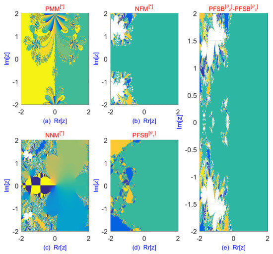
Figure 4.
Dynamical planes of the parallel schemes for solving eigenvalues of Equation (74).
Table 5.
Fractal analysis of the classical and fractional schemes for solving Equation (74).
The enhanced convergence behavior of the classical and fractional parallel schemes is demonstrated through dynamical analysis using fractals, as shown in Table 5 and Figure 4. Fractals of fractional parallel schemes are formed for . In terms of iterations and percentage convergence, the parallel schemes analyzed via fractals exhibit superior convergence behavior compared to existing approaches. Furthermore, fractal analysis plays a crucial role in selecting optimal initial values, allowing for the simultaneous computation of all eigenvalues of the problem.
The numerical results of the proposed scheme for solving the eigenvalue problem (74), using starting values close to the exact eigenvalues, are presented in Table 6. This table clearly demonstrates that the residual error of the scheme is lower compared to the previous method. To evaluate the global convergence behavior of the parallel schemes, we use randomly generated initial vectors produced by MATLAB’s “rand()” function (see Appendix B Table A1). The corresponding numerical results are summarized in Table 7 and Table 8.
Table 6.
Numerical results of parallel schemes using Equation (74).
Table 7.
Memory usage and computation time (C-Time) using random initial values.
Table 8.
Consistency analysis using random initial values for solving Equation (74).
The numerical experiments show that the new proposed technique consistently achieves superior accuracy, numerical stability, and faster performance, especially for large-scale, sparse, or ill-conditioned matrices. In contrast to previous methods, which may suffer from convergence concerns or sensitivity while solving ill-conditioned systems, the novel technique preserves accuracy and stability. In general, the results show that our method is a more stable and efficient solution to complex eigenvalue issues than other analytical methods.
Table 7 and Table 8 demonstrate that the newly developed fractional schemes outperform existing methods when using random initial guess values. This improvement is evident in terms of computational time (C-Time), memory usage (Mem), maximum error (Max-Err), maximum iterations (Max-It), percentage divergence, and the total number of function and derivative evaluations across all iteration steps to solve Equation (74). The approximated roots are computed using 64-digit floating-point algebra, ensuring a high degree of precision for problem simulation. Figure 5 illustrates the residual error when using random initial values, highlighting the superior convergence of the proposed approach compared to existing methods.

Figure 5.
Error graph of the parallel schemes using random initial gusses values for solving (74).
Table 9 provides a detailed theoretical comparison between the newly proposed algorithm and several well-known analytical methods for solving eigenvalue problems, including the QR algorithm (), the Divide-and-Conquer method (), the Generalized Schur Decomposition (), and MATLAB’s built-in function eig() ().
Table 9.
Comparative analysis of eigenvalue computation (74) using analytical and parallel methods.
4.1.4. Analysis of Eigenvalues
- Real eigenvalues: Real eigenvalues indicate stable oscillatory behavior at specific frequencies.
- Complex eigenvalues: The presence of complex eigenvalues suggests damped oscillations, where disturbances gradually decay over time.
4.1.5. Physical Behavioral Interpretation of the Two-Degree-of-Freedom System
- Stable modes: The natural frequencies determine the preferred oscillation modes of the suspension system when disturbed. These modes are crucial for ensuring stability in vehicle dynamics during operation.
- Damping effects: The presence of complex eigenvalues signifies that disturbances will decay over time, leading to a gradual return to equilibrium. This effect is essential for ride comfort, preventing excessive oscillations caused by road irregularities.
- High-frequency response: The highest natural frequency (10.0 Hz) may correspond to the first mode of vibration of the suspension system. This mode is particularly critical for maintaining control and stability at high speeds or during rapid maneuvers.
4.1.6. Case 2: Four-Degree-of-Freedom (4DOF) System
The automotive suspension system is modeled as a four-degree-of-freedom (4DOF) system, representing a more complex vehicle suspension, such as a multi-link suspension. The system consists of two masses representing the car body and two wheel assemblies.
System Parameters
The 4DOF system includes the following mass, damping, and stiffness parameters:
Masses
- kg (car body);
- kg (front-left wheel assembly);
- kg (front-right wheel assembly);
- kg (rear wheel assembly).
Spring Constants
- 80,000 N/m (spring between car body and front axle);
- 60,000 N/m (spring between front axle and ground);
- 60,000 N/m (spring between rear axle and ground).
Damping Coefficients
- 4000 Ns/m (damper between car body and front axle);
- 3000 Ns/m (damper between front axle and ground);
- 3000 Ns/m (damper between rear axle and ground).
Governing Equations
The system’s dynamics are governed by the equation of motion:
where represents the displacement vector
The mass, damping, and stiffness matrices for the 4DOF system are given as
Mass Matrix
Damping Matrix
Stiffness Matrix
To determine the eigenvalues for , we compute the determinant
Expanding the determinant, we obtain
where
The characteristic polynomial is obtained after determinant calculations and simplifications:
The exact eigenvalues of Equation (92), accurate to ten decimal places, are as follows:
The sparsity pattern, symmetry, and conditioning are key structural characteristics of the 2DOF system matrix, as detailed in Table 10.
Table 10.
Characteristics of the eigenvalue problem from a 4DOF mechanical system.
The initial approximations of eigenvalues, close to the exact solutions, are
Dynamical analysis through fractals, as presented in Table 11 and Figure 6, illustrates the improved convergence behavior of both fractional and classical parallel schemes. The fractals of fractional parallel schemes are generated for . In terms of iteration count and percentage convergence, the fractal analysis demonstrates that parallel schemes exhibit superior convergence behavior compared to existing approaches. Moreover, fractal analysis aids in selecting optimal initial values, enabling the simultaneous determination of all eigenvalues in the problem.
Table 11.
Fractal analysis of classical and fractional schemes for solving (92).
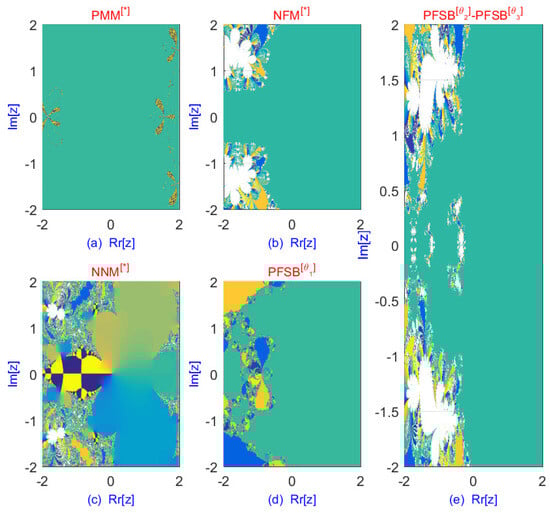
Figure 6.
Dynamical planes of the parallel schemes for solving eigenvalues of (92).
The numerical results of the proposed scheme for solving the eigenvalue problem (92) using initial values close to the exact eigenvalues are presented in Table 12. The data in Table 12 clearly demonstrate that the residual error of the proposed scheme is lower than that of previous methods. To evaluate the global convergence behavior of the parallel schemes, we generate multiple sets of initial vectors using MATLAB’s rand() function (see Appendix B Table A2). The corresponding numerical results, including convergence rates and performance comparisons, are provided in Table 13 and Table 14.
Table 12.
Numerical results of parallel schemes using (92).
Table 13.
Memory usage and computational time (C-Time) using random initial values for solving (92).
Table 14.
Consistency analysis using random initial values for solving (92).
In terms of computational time (in seconds), memory usage, maximum error (see Figure 7), maximum iterations, percentage divergence, and the total number of function and derivative evaluations across all iteration steps for solving (92), Table 13 and Table 14 demonstrate that the newly developed fractional schemes outperform existing methods when using randomly generated initial values. The approximate roots are computed using 64-digit floating-point arithmetic, ensuring a high degree of precision for simulating the problem.
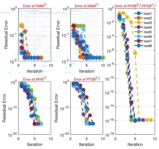
Figure 7.
Error graph of the parallel schemes using random initial guesses values for solving (92).
A detailed theoretical comparison between the newly proposed algorithm and several widely used analytical techniques for solving eigenvalue problems—including the QR algorithm, the Divide-and-Conquer strategy, the Generalized Schur Decomposition, and MATLAB’s built-in function eig() —is presented in Table 15.
Table 15.
Comparative analysis of eigenvalue computation in Equation (92) using analytical and parallel methods.
Simulations demonstrate that the proposed technique consistently achieves higher accuracy, improved numerical stability, and faster performance—particularly for large-scale, sparse, or ill-conditioned matrices—when compared to , , , and , respectively.
4.1.7. Analysis of Eigenvalues for a Four-Degree-of-Freedom Mechanical System
- Stable modes: Real eigenvalues indicate stable modes of oscillation. The frequencies determine how the system naturally oscillates when subjected to disturbances.
- Damped oscillations: Complex eigenvalues signify oscillations that decay over time, representing the damping characteristics of the suspension system. This is crucial for maintaining comfort and ride quality in vehicles.
4.1.8. Physical Interpretation of Eigenvalues in a Four-Degree-of-Freedom System
- Stable modes: The real eigenvalues correspond to natural frequencies ranging from Hz to Hz, where the system exhibits stable oscillations. These modes are critical for ensuring vehicle stability under various loading conditions, particularly when driving over uneven surfaces.
- Damping effects: The presence of complex eigenvalues indicates that the suspension system gradually dissipates energy in response to disturbances, ensuring a smooth return to equilibrium. This characteristic is essential for preventing excessive oscillations that could compromise passenger comfort and vehicle handling.
- Frequency range: The identified natural frequencies define the range of vibrations the suspension system will experience. High-frequency responses (e.g., Hz) correspond to rapid load changes, such as those encountered during cornering or sudden braking.
4.2. Aeroelasticity and Flutter Analysis: Detailed Model and Solution Behavior [35]
Aeroelasticity describes the interaction between aerodynamic forces and structural dynamics, particularly in flexible structures such as aircraft wings, bridges, wind turbine blades, and high-rise buildings. One of the key phenomena studied in aeroelasticity is flutter, a potentially catastrophic oscillatory instability that arises when aerodynamic forces excite the structural modes of a system.
In flutter analysis, the objective is to determine the conditions—such as airspeed or structural stiffness—under which dynamic instability occurs. This is accomplished by solving a coupled system of differential equations that govern the interaction between aerodynamic loads and structural motion. The solution of this system typically reduces to an eigenvalue problem, where the behavior of the eigenvalues indicates whether the system remains stable or becomes unstable.
4.2.1. Flutter Model Overview
Flutter can be modeled using coupled differential equations that describe the interaction between structural and aerodynamic forces acting on a flexible body, such as an aircraft wing. For instance, an airfoil experiencing both bending and torsional motion can be analyzed by formulating equations of motion for structural dynamics and aerodynamic forces governed by potential flow theory.
4.2.2. Equations of Motion
The general form of the structural equations governing the bending and torsional motion of an airfoil is given by
where the following is the case:
- —vertical displacement of the airfoil (bending);
- —angular displacement (torsion);
- m and —mass and moment of inertia of the structure;
- and —damping coefficients;
- and —stiffness coefficients;
- —aerodynamic lift force;
- —aerodynamic pitching moment.
4.2.3. Aerodynamic Forces
The aerodynamic forces, and , depend on the airspeed and the structural motion. For small disturbances, they can be approximated using linearized potential flow theory, leading to the following expressions:
where is the air density, and U is the free-stream airspeed. The aerodynamic forces are coupled to the structural equations, resulting in an interaction between the two modes: bending and torsion.
By selecting specific parameter values, we define the following:
- kg—mass per unit length of the wing;
- kg·m2—moment of inertia of the wing;
- Ns/m—damping coefficient for bending;
- Ns·m/rad—damping coefficient for torsion;
- N/m—bending stiffness;
- Nm/rad—torsional stiffness.
The aerodynamic forces acting on the wing are modeled as linearized functions of the displacements and are computed for the following conditions:
- kg/m3—air density;
- m2—wing surface area.
Using the parameter values in Equation (95), we obtain the following system of coupled differential equations:
These equations describe the bending displacement and torsional rotation . The aerodynamic coupling terms, and , establish the interaction between the bending and torsional motions. This coupling highlights the crucial role of the airspeed U in determining the stability of the system.
4.2.4. Coupled System and Eigenvalue Problem
The governing equation of motion for the aeroelastic system is given by
where the state vector is defined as
The mass matrix , damping matrix , and stiffness matrix are given by
To determine the flutter speed and assess the stability of the system, we assume a solution of the form
where represents the oscillation frequency. Substituting this assumption into Equation (98) leads to the following eigenvalue problem:
The characteristic equation for the eigenvalues is obtained by computing the determinant:
This equation governs the natural frequencies and damping characteristics of the system as a function of the airspeed U, providing insights into the system’s stability and the onset of flutter.
Next, we solve the system at a low airspeed, specifically . Substituting this value into Equation (103) yields
The corresponding characteristic polynomial is given by
The sparsity pattern, symmetry, and conditioning are key structural characteristics of the 2DOF system matrix, as detailed in Table 16. Table 17 shows the parameter and values in the proposed scheme for solving Equation (105), derived from the dynamical plane analysis, indicating a wider and faster convergence region.
Table 16.
Characteristics of the eigenvalue problem from a 2DOF mechanical system.
Table 17.
Values of and in the proposed methods for solving Equation (105).
The exact eigenvalues, computed up to ten decimal places, are
The initial eigenvalues, chosen close to the exact roots, are
The dynamical analysis and fractals, as presented in Table 18 and Figure 8, illustrate the improved convergence behavior of both fractional and classical parallel schemes. The fractal patterns of fractional parallel schemes are generated for , highlighting their enhanced stability and efficiency. In terms of iteration count and percentage convergence, the fractal analysis demonstrates that parallel schemes outperform existing methods, providing superior convergence behavior. Additionally, fractal analysis plays a crucial role in selecting optimal initial values, facilitating the simultaneous computation of all eigenvalues in the system.
Table 18.
Fractal analysis of classical and fractional schemes for solving Equation (105).
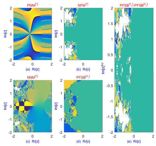
Figure 8.
Dynamical planes of the parallel schemes for solving the eigenvalues of Equation (105).
The numerical results of the proposed numerical scheme for solving the eigenvalue problem (105) using initial values close to the exact eigenvalues are presented in Table 19. As illustrated in Table 19, the scheme exhibits a lower residual error compared to previous methods, as shown in Figure 9. Matlab’s Rand() function is used to generate a set of random initial vectors (see Appendix B Table A3), which are then utilized to compute the rate of convergence and assess the global convergence behavior of the parallel schemes. The corresponding numerical results are summarized in Table 20 and Table 21.
Table 19.
Numerical results of parallel schemes using Equation (105).
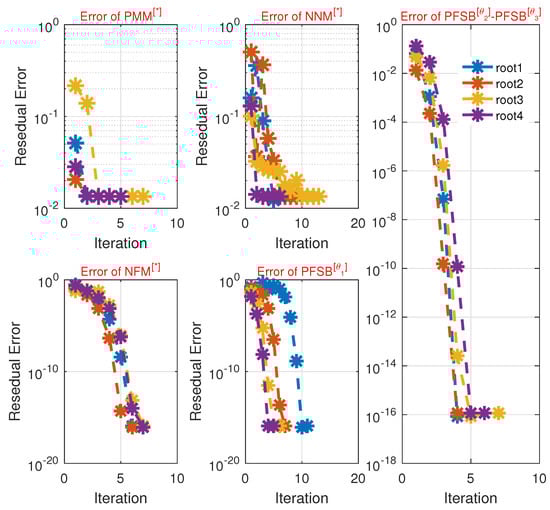
Figure 9.
Error graph of the parallel schemes using random initial guesses for solving Equation (105).
Table 20.
Memory usage and computational time (C-Time) for different schemes using random initial values for solving Equation (105).
Table 21.
Consistency analysis using random initial values for solving Equation (105).
The newly developed fractional schemes demonstrate superior performance compared to existing methods when using random initial guesses, as shown in Table 20 and Table 21. This improvement is evident when evaluating key computational metrics such as execution time (in seconds), memory usage, maximum error, maximum iterations, percentage divergence, and the number of function and derivative evaluations across all iteration steps required to solve (105). The approximated roots are computed using 64-digit floating-point arithmetic, ensuring a high degree of precision in simulating the problem.
The theoretical comparison between the newly developed parallel approach and several analytical techniques—including the QR algorithm, the Divide-and-Conquer strategy, the Generalized Schur Decomposition, and MATLAB’s eig() function—is presented in Table 22.
Table 22.
Comparative analysis of eigenvalue computation in Equation (105) using analytical and parallel methods.
Our proposed approach outperforms conventional techniques in terms of accuracy, stability, and the handling of sparse or ill-conditioned matrices, as demonstrated by the numerical results. These findings highlight the effectiveness and reliability of the newly developed strategy for solving difficult eigenvalue problems.
4.2.5. Solution Behavior and Physical Interpretation
- Stable regime (below flutter speed): For , the system remains stable. The real parts of all eigenvalues are negative, indicating that oscillations decay over time due to damping. The system naturally returns to equilibrium after disturbances, ensuring structural stability.
- Flutter point (at critical speed): At , the system reaches a marginally stable state. The real part of one pair of eigenvalues approaches zero, meaning that the damping effect vanishes. Oscillations neither grow nor decay, marking the flutter onset speed. Beyond this point, the wing loses its ability to return to a stable state once disturbed.
- Unstable regime (above flutter speed): For , the real part of at least one pair of eigenvalues becomes positive, leading to exponentially growing oscillations. This marks the onset of the flutter regime, where both bending and torsional oscillations increase uncontrollably, potentially causing structural failure unless corrective action, such as reducing airspeed, is taken.
4.3. Limitations of Fractional-Order Parallel Schemes for Eigenvalue Problems
The proposed fractional-order parallel techniques offer a strong framework for tackling complex eigenvalue problems while improving convergence behavior. By integrating fractional dynamics and parallel iteration, these methods estimate all eigenvalues with high accuracy. Their efficiency is particularly apparent in high-degree and complex eigenvalue problem, where existing schemes may not work well. Here are some limitations of the proposed fractional-order parallel scheme:
- The techniques can perform worse on matrices with clustered or closely spaced eigenvalues, resulting in slower convergence or instability.
- Optimal convergence and higher accuracy require reasonable initial approximations, which are difficult to produce for nonsymmetric or ill-conditioned matrices.
- The inclusion of fractional-order terms increases computing time, especially for sparse or nontrivially large matrix problems.
- Optimal initialization using fractal analysis is problem-specific and does not provide generic automation.
- Implementation and visualization may require significant computational power and expertise.
To improve the proposed fractional-order parallel algorithms, future studies should focus on memory-reducing fractional operators, GPU/multicore parallelization for large-scale problems, and adaptive parameter adaption using machine learning or optimization techniques. Effective initialization strategies, as well as hybrid methods using error estimators, will improve accuracy and reliability. In addition, theoretical extensions to nonlinear systems and fractional PDEs will increase when utilizing the technique and scope.
5. Conclusions
In this work, we developed novel fractional-order numerical methods for computing single eigenvalues and extended them into parallel schemes capable of determining all eigenvalues simultaneously. The proposed – schemes achieve a theoretical convergence order of , demonstrating their efficiency and accuracy in solving eigenvalue problems. Numerical experiments confirm that the proposed fractional schemes outperform existing methods, including , , and , particularly when initialized with accurate eigenvalue estimates. The computational efficiency of these fractional parallel schemes is evident in their reduced number of arithmetic operations, making them more suitable for large-scale applications. Dynamical analysis highlights that the percentage of convergence zones in fractal structures is significantly improved, effectively identifying optimal initial eigenvalue estimates for parallel computations. Furthermore, the fractional methods demonstrate strong global convergence properties, exhibiting robustness even for random initial values. In terms of computational cost and accuracy, the fractional methods outperform existing numerical solvers across multiple metrics, including memory usage, residual error, function and derivative evaluations, iteration count, and convergence–divergence behavior. These findings establish fractional-order parallel schemes as highly efficient and reliable alternatives for solving eigenvalue problems in scientific computing, engineering, and applied mathematics.
Future research may focus on optimizing parameter selection, extending the approach to generalized eigenvalue problems, and investigating real-world applications such as quantum mechanics, stability analysis, and computational fluid dynamics. The strong numerical performance of fractional-order methods suggests significant potential for further advancements in large-scale numerical computations.
Author Contributions
Conceptualization, M.S. and B.C.; methodology, M.S.; software, M.S.; validation, M.S.; formal analysis, B.C.; investigation, M.S.; resources, B.C.; writing—original draft preparation, M.S. and B.C.; writing—review and editing, B.C.; visualization, M.S. and B.C.; supervision, B.C.; project administration, B.C.; funding acquisition, B.C. All authors have read and agreed to the published version of the manuscript.
Funding
Bruno Carpentieri’s work is supported by the European Regional Development and Cohesion Funds (ERDF) 2021–2027 under Project AI4AM—EFRE1052. He is a member of the Gruppo Nazionale per il Calcolo Scientifico (GNCS) of the Istituto Nazionale di Alta Matematica (INdAM), and this work was partially supported by INdAM-GNCS under the Progetti di Ricerca 2024 program.
Data Availability Statement
Data are contained within the article.
Conflicts of Interest
The authors declare no conflicts of interest.
Notations
| CPU-time | Computational time seconds |
| Max-It | Maximum iterations |
| Max-Err | Maximum error |
| Per-Convergence | Percentage convergence |
| Existing parallel methods | |
| Residual error | |
| Newly developed methods |
Appendix A
Appendix A.1
Theorem A1.
Suppose that for , where . Then, the Generalized Taylor Formula [36] is given by
where
and
- Consider the Taylor expansion of around as
- Factoring out , we obtainwhere
- Around , the Caputo-type derivative of is given by
- These expansions are used to analyze the convergence of the methods.
Appendix A.2
The coefficients of were used in the proof of Theorem 2.
Appendix B
The random initial starting vector is used in Eigenvalue Problem 1 to demonstrate the global convergence of numerical techniques, as shown in Appendix B and Table A1.
Table A1.
Random starting vectors in parallel schemes.
Table A1.
Random starting vectors in parallel schemes.
| Ran-Test | ||||
|---|---|---|---|---|
| 1 | ||||
| 2 | ||||
| 3 | ||||
| 5 |
The random initial starting vector is used in Eigenvalue Problem 1 to demonstrate the global convergence of numerical techniques, as shown in Appendix B and Table A2.
Table A2.
Random initial vectors for fractional and classical schemes.
Table A2.
Random initial vectors for fractional and classical schemes.
| Ran-Test | ||||||||
|---|---|---|---|---|---|---|---|---|
| 1 | ||||||||
| 2 | ||||||||
| 3 | ||||||||
| 5 |
The random initial starting vector is used in Eigenvalue Problem 1 to demonstrate the global convergence of numerical techniques, as shown in Appendix B Table A3.
Table A3.
Random starting vectors in parallel schemes.
Table A3.
Random starting vectors in parallel schemes.
| Ran-Test | ||||
|---|---|---|---|---|
| 1 | ||||
| 2 | ||||
| 3 | ||||
| ⋮ |
References
- Guglielmi, N.; De Marinis, A.; Savostianov, A.; Tudisco, F. Contractivity of neural ODEs: An eigenvalue optimization problem. Math. Comput. 2025. [Google Scholar]
- Meng, F.; Wang, Z.; Zhang, M. Pissa: Principal singular values and singular vectors adaptation of large language models. Adv. Neural Inf. Process. Syst. 2024, 37, 121038–121072. [Google Scholar]
- Ciftci, H.; Hall, R.L.; Saad, N. Construction of exact solutions to eigenvalue problems by the asymptotic iteration method. J. Phys. A Math. Gen. 2005, 38, 1147. [Google Scholar]
- Zhang, Y.; Chen, C.; Ding, T.; Li, Z.; Sun, R.; Luo, Z. Why transformers need adam: A hessian perspective. Adv. Neural Inf. Process. Syst. 2024, 37, 131786–131823. [Google Scholar]
- Ramond, P. The Abel–Ruffini theorem: Complex but not complicated. Am. Math. Mon. 2022, 129, 231–245. [Google Scholar]
- Gidiotis, A.; Tsoumakas, G. A divide-and-conquer approach to the summarization of long documents. IEEE/ACM Trans. Audio Speech Lang. Process. 2020, 28, 3029–3040. [Google Scholar] [CrossRef]
- Goldstine, H.H.; Murray, F.J.; Von Neumann, J. The Jacobi method for real symmetric matrices. J. ACM (JACM) 1959, 6, 59–96. [Google Scholar]
- Fokkema, D.R.; Sleijpen, G.L.; Van der Vorst, H.A. Jacobi–Davidson style QR and QZ algorithms for the reduction of matrix pencils. SIAM J. Sci. Comput. 1998, 20, 94–125. [Google Scholar]
- Lu, Z.; Niu, Y.; Liu, W. Efficient block algorithms for parallel sparse triangular solve. In Proceedings of the 49th International Conference on Parallel Processing, Edmonton, AB, Canada, 17–20 August 2020; pp. 1–11. [Google Scholar]
- Zhang, Z.; Wang, H.; Han, S.; Dally, W.J. Sparch: Efficient architecture for sparse matrix multiplication. In Proceedings of the 2020 IEEE International Symposium on High Performance Computer Architecture (HPCA), San Diego, CA, USA, 22–26 February 2020; pp. 261–274. [Google Scholar]
- Bašić, J.; Blagojevixcx, B.; Baxsxixcx, M.; Sikora, M. Parallelism and Iterative bi-Lanczos Solvers. In Proceedings of the 2021 6th International Conference on Smart and Sustainable Technologies (SpliTech), Split & Bol, Croatia, 8–11 September 2021; pp. 1–6. [Google Scholar]
- Wu, G.; Wei, Y. A Power–Arnoldi algorithm for computing PageRank. Numer. Linear Algebra Appl. 2007, 14, 521–546. [Google Scholar]
- Nourein, A.W. An improvement on Nourein’s method for the simultaneous determination of the zeroes of a polynomial (an algorithm). J. Comput. Appl. Math. 1977, 3, 109–112. [Google Scholar]
- Falcão, M.I.; Miranda, F.; Severino, R.; Soares, M.J. Weierstrass method for quaternionic polynomial root-finding. Math. Methods Appl. Sci. 2018, 41, 423–437. [Google Scholar]
- Kipouros, T.; Jaeggi, D.; Dawes, B.; Parks, G.; Savill, M.A.; Clarkson, P.J. Insight into high-quality aerodynamic design spaces through multi-objective optimization. CMES Comput. Model. Eng. Sci. 2008, 37, 1–23. [Google Scholar]
- Landman, D.; Simpson, J.; Vicroy, D.; Parker, P. Response surface methods for efficient complex aircraft configuration aerodynamic characterization. J. Aircraf. 2007, 44, 1189–1195. [Google Scholar]
- Liu, Y. Bibliometric Analysis of Weather Radar Research from 1945 to 2024: Formations. Develop. Trends Sens. 2024, 24, 3531. [Google Scholar]
- Jajarmi, A.; Baleanu, D. A new iterative method for the numerical solution of high-order non-linear fractional boundary value problems. Front. Phys. 2020, 8, 220. [Google Scholar]
- Sazaklioglu, A.U. An iterative numerical method for an inverse source problem for a multidimensional nonlinear parabolic equation. Appl. Numer. Math. 2024, 198, 428–447. [Google Scholar]
- Akgül, A.; Cordero, A.; Torregrosa, J.R. A fractional Newton method with 2αth-order of convergence and its stability. Appl. Math. Lett. 2019, 98, 344–351. [Google Scholar]
- Batiha, B. Innovative Solutions for the Kadomtsev–Petviashvili Equation via the New Iterative Method. Math. Prob. Eng. 2024, 2024, 5541845. [Google Scholar]
- Weierstrass, K. Neuer Beweis des Satzes, dass jede ganze rationale Function einer Verän derlichen dargestellt werden kann als ein Product aus linearen Functionen derselben Verän derlichen. Sitzungsberichte KöNiglich Preuss. Akad. Der Wiss. Berl. 1981, 2, 1085–1101. [Google Scholar]
- Nedzhibov, G.H. Inverse Weierstrass–Durand–Kerner Iterative Method. Int. J. Appl. Math. 2013, 28, 1258–1264. [Google Scholar]
- Nourein, A.W.M. An improvement on two iteration methods for simultaneous determinationof the zeros of a polynomial. Int. J. Comput. Math. 1977, 6, 241–252. [Google Scholar]
- Zhang, X.; Peng, H.; Hu, G. A high order iteration formula for the simultaneous inclusion of polynomial zeros. Appl. Math. Comput. 2006, 179, 545–552. [Google Scholar]
- Petkovic, M. Iterative Methods for Simultaneous Inclusion of Polynomial Zeros; Springer: Berlin/Heidelberg, Germany, 2006; Volume 1387. [Google Scholar]
- Zein, A. A general family of fifth-order iterative methods for solving nonlinear equations. Eur. J. Pure Appl. Math. 2023, 16, 2323–2347. [Google Scholar]
- Halilu, A.S.; Waziri, M.Y. A transformed double step length method for solving large-scale systems of nonlinear equations. J. Numer. Math. Stochastics 2021, 9, 20–23. [Google Scholar]
- Rafiq, N.; Akram, S.; Shams, M.; Mir, N.A. Computer geometries for finding all real zeros of polynomial equations simultaneously. Comput. Mater. Contin. 2021, 69, 2636–2651. [Google Scholar]
- Petković, M.S.; Petković, L.D.; Džunić, J. On an efficient simultaneous method for finding polynomial zeros. Appl. Math. Lett. 2014, 28, 60–65. [Google Scholar]
- Wang, D.R.; Wu, Y.J. Some modifications of the parallel Halley iteration method and their convergence. Computing 1987, 38, 75–87. [Google Scholar]
- Petković, M.S.; Rančić, L.; Milošević, M. The improved Farmer–Loizou method for finding polynomial zeros. Int. J. Comput. Math. 2012, 89, 499–509. [Google Scholar]
- Gillespie, T. Fundamentals of Vehicle Dynamics; SAE: Warrendale, PA, USA, 2000. [Google Scholar]
- Reimpell, J.; Stoll, H.; Betzler, J. The Automotive Chassis: Engineering Principles; Elsevier: Amsterdam, The Netherlands, 2001. [Google Scholar]
- Prohl, M.A. A general method for calculating critical speeds of flexible rotors. J. Appl. Mech. 1945, 12, A142–A148. [Google Scholar]
- Shams, M.; Carpentieri, B. On highly efficient fractional numerical method for solving nonlinear engineering models. Mathematics 2023, 11, 4914. [Google Scholar] [CrossRef]
Disclaimer/Publisher’s Note: The statements, opinions and data contained in all publications are solely those of the individual author(s) and contributor(s) and not of MDPI and/or the editor(s). MDPI and/or the editor(s) disclaim responsibility for any injury to people or property resulting from any ideas, methods, instructions or products referred to in the content. |
© 2025 by the authors. Licensee MDPI, Basel, Switzerland. This article is an open access article distributed under the terms and conditions of the Creative Commons Attribution (CC BY) license (https://creativecommons.org/licenses/by/4.0/).