Abstract
In this paper, we propose an approach for constructing quasiparticle-like asymptotic solutions within the weak diffusion approximation for the generalized population Fisher–Kolmogorov–Petrovskii–Piskunov (Fisher–KPP) equation, which incorporates nonlocal quadratic competitive losses and a fractal time derivative of non-integer order (, where ). This approach is based on the semiclassical approximation and the principles of the Maslov method. The fractal time derivative is introduced in the framework of calculus. The Fisher–KPP equation is decomposed into a system of nonlinear equations that describe the dynamics of interacting quasiparticles within classes of trajectory-concentrated functions. A key element in constructing approximate quasiparticle solutions is the interplay between the dynamical system of quasiparticle moments and an auxiliary linear system of equations, which is coupled with the nonlinear system. General constructions are illustrated through examples that examine the effect of the fractal parameter () on quasiparticle behavior.
Keywords:
fractals; fractal derivatives and integrals; nonlocal Fisher–KPP equation; semiclassical approximation; quasiparticles; Maslov method MSC:
28A80; 26A33; 81Q20; 92D25
1. Introduction
The modeling of reaction–diffusion (RD) systems serves as a fundamental theoretical framework for studying nonlinear phenomena across diverse fields, including physics, chemistry, biology, and engineering [1]. To accurately describe RD processes in complex physical and biological systems exhibiting anomalous diffusion and memory effects, a fractal derivative with respect to time is often introduced in the mathematical formulation.
Diffusion processes in fragmented media, as well as under random external influences, are characterized by complexity and diversity of dynamics. In systems with internal multiscale geometric or physical inhomogeneities, diffusion deviates from the standard behavior described by Fick’s law and is, instead, classified as anomalous diffusion (AD). In nonlinear processes occurring in physical and biological systems, AD plays a fundamental role and has been extensively studied. Numerous authors have contributed to the field, and there is a wealth of excellent reference books and reviews available on the topic. We do not aim to provide a comprehensive review here; instead, we refer to a relatively recent work [2]. This review includes, among other things, a historical overview of the topic and a detailed discussion of applications of AD models to fundamental problems in nonlinear physics, such as turbulence and random walks. It also examines the physical mechanisms underlying fractional AD, which are described using diffusion equations with fractional time derivatives. Models of complex nonlinear phenomena in biological systems involving fractional analysis have been discussed in detail in previous reviews [3,4]. It is important to note that fractional derivatives are nonlocal operators acting on continuous and differentiable functions of continuous variables. While they are not defined directly on fractals, they indirectly capture the fractal properties of the modeled system through the fractional order of the derivative, which reflects the system’s fractal dimension.
Over the past few decades, the development of fractal calculus has enabled the direct formulation of model equations for physical and biological processes and systems in terms of fractal operators, such as derivatives and integrals, much like in ordinary calculus. The basic concepts of fractal calculus are outlined, for instance, in [5,6,7]. Subsequent works [8,9] explored local and nonlocal aspects of the basic constructions of fractal calculus, and the relationship between the fractal derivative and the fractional Caputo derivative was discussed in [10]. A comprehensive review of fractal analysis, including recent developments and applications, is available in [11] and the references therein.
These advancements have sparked a growing interest in research into physical phenomena on fractal objects, as partially demonstrated in [9,11]. In particular, fractal calculus provides an adequate framework for simulating the dynamics of reaction–diffusion (RD) systems in media with complex properties and irregular influences.
The emergence of model equations incorporating fractal operators poses significant challenges for the development of methods to analyze these equations and to obtain both exact and approximate solutions.
In the study of biological populations comprising a single species, the classical Fisher–Kolmogorov–Petrovskii–Piskunov (Fisher–KPP) equation of the RD type that accounts for local competitive losses was introduced in [12,13] to describe population waves. Incorporating nonlocal competitive losses, which enable long-range interactions within the population [1], expands the range of dynamic regimes that can be modeled.
A recent review [14] presented the state of the art in the study of nonlocal RD models in biological systems across multiple scales, including microbiological populations and neural fields. Notably, the nonlocal Fisher–KPP equation has been incorporated into models of cancer cell dynamics. The modified Fisher–KPP equation with nonlocal competitive losses provides a framework for describing the formation and evolution of patterns in single-species populations. Similar nonlocal kinetic models have been primarily studied through numerical simulations (e.g., [1,15,16]). Analytical methods have been developed under appropriate approximations. The formalism for constructing asymptotic solutions within the weak diffusion approximation was developed in [17,18,19] for the nonlocal Fisher–KPP equation, which includes the standard first-order time derivative:
In [20], examples of asymptotic solutions to Equation (1) constructed within the framework of this method were presented.
Here, the equation is written in dimensionless form, a real smooth function () is the population density, and as ; , , and ; and are infinitely smooth, increasing functions, as no faster than polynomially; and is a real nonlinearity parameter. The term stands for the nonlocal competition losses and is characterized by an influence function (), coefficient stands for the reproduction rate, and is the diffusion coefficient. In the case of local competitive losses, the integral term in Equation (1) is replaced by .
In [21], the approach developed in [17,18], which utilizes the Maslov method (see, e.g., Refs. [22,23]), was generalized to construct asymptotic solutions for Equation (1) in the form of two quasiparticles. These solutions characterize the dynamics of interacting local modes of population density.
In this paper, we extend the formalism developed in [17,18,19,21] to the nonlocal Fisher–KPP equation with a fractal time derivative of fractional order . Within the weak diffusion approximation, we derive asymptotic solutions that capture the fractal dynamics of quasiparticles. Preliminary results were presented in [24].
Note that the concepts and techniques of the Maslov method, originally developed in quantum theory, have found broad applications in a range of linear and nonlinear mathematical physics problems. For further details, refer to [21,22,23], along with the references therein. However, this approach has not been previously applied to problems involving fractal dynamics.
Fractional powers in dimensional indices emerge when describing fractal media. In such media, unlike in continuous media, a randomly walking particle can move away from its starting point more slowly because not all directions of motion are accessible—only those aligned with the fractal structure (e.g., on a plane or in space). The slowdown of diffusion in fractal media may manifest itself in such a way that physical quantities evolve more slowly than the first space derivative would suggest. This effect can be captured either through an integro-differential equation involving a fractional-order space derivative or, more logically, by directly employing a fractal derivative defined explicitly on the fractal structure. In the case of temporal fractality, the random motion of a particle occurs, in a certain sense, in a jumpy manner at moments associated with the fractal time interval. This behavior might be expected to accelerate diffusion.
The properties of fractional derivatives, which reflect the “memory” characteristics of a process, and fractal derivatives, which characterize local self-similarity, have been extensively discussed and applied to RD-type equations, including the Fisher–KPP equation, in numerous publications, such as [25,26,27], as well as in recent works, for example, [11,28,29].
The relationship between the Caputo fractional derivative commonly used in the Fisher–KPP model (e.g., [28]) and the fractal derivative, as defined in [5,6], was examined in [10]. The authors showed that the Caputo derivative can be interpreted as a continuous approximation of the fractal derivative. Moreover, the derivative of a fractional function under this approximation yields a Caputo-like form. Based on this observation, we may conjecture that fractional and fractal derivatives both capture essential aspects of fractal dynamics and can be viewed as complementary. This motivates the study of the Fisher–KPP equation with a fractal time derivative within the framework of calculus [5,6,11], where the parameter represents the fractal dimension of a domain (F) associated with variation in the independent variable.
The structure of this paper is outlined as follows: Section 2 provides a brief overview of the necessary basic concepts and notations from fractal calculus and introduces the nonlocal Fisher–KPP equation with a fractal time derivative. In Section 3, we introduce the class of trajectory-concentrated functions in which asymptotic solutions are sought. A definition of quasiparticles is provided, and the Fisher–KPP equation under consideration is decomposed into a system of equations describing the fractal dynamics of interacting quasiparticles. In Section 4, we derive estimates for operators in the class of trajectory-concentrated functions and introduce the moments that characterize quasiparticles. Expansions of the coefficients of the operators in the equation are performed within this function class. In Section 5, we derive a fractal dynamical system for the moments of quasiparticles and discuss its properties. Using the general solution of the dynamical system of moments, in Section 6, we introduce a system of linear equations with a fractal time derivative associated with the equations for quasiparticles. In Section 7, we explore the relationship between the Cauchy problem for the fractal nonlocal Fisher–KPP equation and the associated linear system under certain conditions. In the asymptotic approximation, we derive the Green function for the associated linear system, which generates approximate solutions to the original nonlinear system describing the quasiparticles. In Section 8, we illustrate the general results with examples of the dynamics of two quasiparticles and examine the influence of the fractal derivative parameter on quasiparticle dynamics. In Section 9, we provide our concluding remarks.
2. Fisher–KPP Equation with Fractal Time Derivative
In Equation (1), we assume that time (t) does not evolve continuously but, rather, on a fractal set (, where (with ) is a closed interval of the real line ()). In this context, the time derivative () in (1) must be replaced by an appropriate time derivative on F. To accomplish this, we employ the calculus, as developed in [5,6], with additional insights from [11]. For the fractal set (F) we consider a Cantor set (see, e.g., [5,6,11] and recent works [10,30,31]). Here, we provide a brief overview of the calculus, primarily following [5,6,31].
The indicator (flag) function of the set (F) and is given as
Let , , , , , be a partition of the interval (I).
For a parameter () and partitions () of I, the coarse-grained mass function () is given by the following expression:
and the Hausdorff mass measure is defined as
The infimum in (3) is taken over all partitions () of the interval (I), and is Euler’s Gamma function. Then, the fractal (γ) dimension of the set (F) (the value of at which is finite) is defined by the following condition:
For a fixed number (), the integral staircase function () on F is defined as
The function increases monotonically with x, , is continuous on , and is a constant in when .
For a function (, ) and , the number (l) is termed the F limit of the function (f) through the set (F) as , , if , there exists such that when [5]. The following notation is used: .
The function (f) is F-continuous at the point () if . Note that F continuity is not defined for .
Using the integral staircase function () for the set (F), we can introduce the important concept of an -perfect set. This set can be constructed algorithmically for F and represents its essential fractal properties. For -perfect set F, the following property holds: if , then is different from at all points (y) on at least one side of x (see [5] for details). This property makes it possible to define the derivative on a fractal set. An example of an -perfect set is the middle Cantor set for , where is the Hausdorff dimension of —in particular, for the -middle Cantor set (dim ) (e.g., [11]).
For a perfect set (F) and a function (f), the derivative of f at x is defined as [5]
when the F limit exists.
Some basic rules for -differentiation are given below following [5].
The derivative of a constant function is zero: if , c is a real constant, , then .
The derivative of the integral staircase function (, ) is the characteristic function () of F:
Let f and g be functions defined on , and suppose derivatives and exist for all ; then, the following properties hold.
Linearity: Derivatives and exist, where c is a constant. Moreover, and .
Leibniz rule: Derivative exists and satisfies
Chain rule: The chain rule for the fractal derivative is expressed as follows (see [32]):
In particular, .
Let denote the class of bounded functions on F. Next, to introduce the integral of a function () on , the following definitions are used (see, e.g., [5,11]):
The upper sum () and the lower sum () over the subdivision () of the interval (I) for a function () and the finite function (, ) are given by the following expressions:
Then, the -integral of a function () is defined as
If the integral (13) exists, the function () is called -integrable on .
The -integral has the obvious property of linearity, and . Below, we present some basic properties that characterize the specifics of the integral (see [5] for details).
For a continuous and -differentiable function (), there exist an -perfect set (F) and F-continuous function () such that , and the following equality holds:
Also, we have
3. Trajectory-ConcentratedFunctions and Decomposition of the Equation
We investigate the influence of time fractality on the dynamics described by Equation (17). Specifically, we analyze the asymptotic solutions of Equation (17) under the weak diffusion approximation, considering the parameter as a small asymptotic parameter ().
Let and be -continuous and -differentiable real functions of t in the sense of calculus (Section 2) that regularly depend on as , , . The dependence on t in the and functions is mediated by the integral staircase function ().
Asymptotic solutions for Equation (17), as well as for Equation (1), can be constructed in the limit as within the framework of the so-called trajectory concentrated functions (TCFs) [18,19]. The class () of these functions is defined by its common element as follows:
where , ; real functions and are functional parameters of the class, regularly depends on as , and belongs to the Schwartz space with respect to the argument ().
The functions of the class are localized within a neighborhood of a point that moves in the phase space of a dynamical system associated with the moments of the equation solution. Furthermore, characterizes the spatial trajectory of this point (for details, see [17,18]).
We also note that the class of trajectory-concentrated functions has previously been used in quantum mechanics (see [33] and references therein). In this context, approximate solutions of quantum equations constructed within this class are interpreted as semiclassical solutions. By analogy, we adopt this terminology for the Fisher–KPP Equations (1) and (17).
To construct quasiparticle solutions to Equation (17), we employ a collection of the classes, i.e.,
with functional parameters and . Here, , and K denotes the number of quasiparticles. The function corresponds to the trajectory of the s-th quasiparticle.
We seek a solution to Equation (17) in the form of
where functions are governed by the following equations:
The summation of Equation (21) yields Equation (17) for the function defined in (20). Notably, the function in (20) cannot be regarded as a superposition of the functions, since these functions are interdependent. Here, represents the s-th quasiparticle. Accordingly, we refer to Equation (21) as the quasiparticle decomposition system (QDS) for K quasiparticles.
Next, to construct a solution to Equation (17), we define estimates of corresponding operators in the classes.
4. Estimates of Operators and Moments
In accordance with [17,18,21], an operator () acting on functions () from the class are estimated as if
where is the norm of .
From Equation (22), we directly obtain the following estimates for the products and powers of operators and :
and, in particular,
just as in the case of Equation (1) [17,18,21].
Note that we cannot directly obtain an estimate for the time-derivative operator () in Equation (21) within the class when functional parameters and are arbitrary. However, an estimate can be obtained for a “prolonged” time-derivative operator:
which accounts for both the structure of functions from class and the properties of the derivative (), such as linearity, the Leibniz rule (9), and the properties of the chain rule (10).
4.1. The Moments
For functions () belonging to the class, we define the moments as
which exist by virtue of the definitions (18) and (19) of .
Here, and are the zeroth-order and first-order moments, respectively, and is the l-th central moment of . We also impose the following condition on the functional parameter () of the class [17,18,21]:
Then, the function is concentrated in the space neighborhood of the curve expressed as . The second moment () characterizes the relative deviation of normalized to .
To simplify the notation, we drop the dependence on the variables and the subscript in what follows, which avoids confusion. Specifically, we write , , .
Setting in (27), we have
4.2. Expansion of Equation Coefficients
To construct asymptotic solutions to Equation (17), we expand the and coefficients into formal power series in the neighborhood of the trajectory () [18,21]:
where , and
For the coefficients of the expansions in (32), we use the simplified notations of , , and .
The solution u to Equation (17) within the semiclassical framework is characterized by its asymptotic expansion in powers of . The leading term and the first two corrections in this expansion describe the essential features of the solution with an accuracy of (see [17,18,19]). To construct explicit analytical expressions for these asymptotic terms, the zeroth-order moment (), the first-order moment (), and the second-order moment () are computed, each with an accuracy of .
Given this, the analysis can be limited to equations for moments up to the second order, as higher-order moments do not contribute to the solution at the desired level of accuracy. This simplification aligns with the semiclassical approach, where higher-order terms in the asymptotic series are typically negligible for practical purposes.
5. The Dynamical System of Moments
Let us apply derivative to in Equation (27) and substitute , where , into the right-hand side of the relation obtained from Equation (21). This yields
Consider in a neighborhood of the trajectory expressed as . Expand in terms of and using expansions (31) and (32), along with Equation (27). Then, for the case of , we can express (34) as a formal series:
In view of estimates (24), (29), and (30), expansion (35) can be written accurately for as
where , ; ; , . Then, according to (36), we have
Here, we keep in mind that , , and .
Equation (41) and similar equations can be treated as approximations with a specified accuracy in , provided we restrict ourselves to a finite number of terms in the infinite sums of (41) while considering the estimates (29).
By neglecting terms of order and higher in Equation (41) and incorporating (38), we derive the following evolution equation for , which includes moments up to the second order:
By applying the derivative operator () to the first-order moment () and carrying out the necessary calculations, we arrive at the following equation:
Then, we have
Using expression (39), we obtain the following evolutionary equation for , which includes moments up to the second order:
Similarly, the equations for higher-order moments are derived in the following form:
By neglecting terms of order and higher in Equation (46), we derive the following evolution equation for the second-order moment ():
We observe that the dynamical system of moments defined by Equations (41), (45), and (47) characterizes the localization trajectory of an asymptotic solution (u) to Equation (17). This solution is found with an accuracy of within the class of functions () in the form of (18) (see, for example, [17,18]).
5.1. The Fractal Einstein–Ehrenfest System of the Second Order
Consider Equations (42), (45), and (47) as templates and introduce a dynamical system where the variables are not moments of the solutions () to the nonlinear system (21).
Let
be a vector consisting of functions , , and , which are not moments of any function (). We assume that the functions (48) are -differentiable in the sense of the definition (7).
Let us replace moments , , and in Equations (42), (45), and (47) with the corresponding functions (48). Then, we obtain the following dynamical system for functions (48):
5.2. On the “Prolongation” of the Fractal Time Derivative
When constructing asymptotic solutions to Equation (21) within the classes (19), it is more convenient to apply estimates of the operators (22) defined not on arbitrary functions () from the class (19) but on solutions () of Equation (21) with .
In this case, the estimates (24) for operators and remain unchanged. However, the functional parameter (), as determined by (28), is governed by Equation (45) (or (44)), from which it follows that . Thus, the operator (), which is included in the “prolonged” operator () in the form of (25), receives the estimate (), which exceeds the estimate (26) for the operator (). This allows us to simplify the “prolonged” operator () by removing the operator without violating the estimate for .
Additional simplifications are obtained by imposing the following condition on the functional parameter () from the class (19):
Thus, in what follows, instead of the operator () in the form of Equation (25), we use the simplified “prolonged” fractal time-derivative operator, i.e,
with and estimate of
6. Associated Fractal Linear Equations
Consider the nonlinear system of Equation (21), along with expansions (31), (32), and (35) in the following form:
Let us derive the linear system of equations associated with an approximate nonlinear system (56), where a finite number of terms is retained in the formal sums based on estimates (23), (26), and (29).
To achieve this, we restrict ourselves to moments up to the second order and replace moments , , and in Equation (56) with the corresponding functions (, , and , respectively) from the general solution (52) of the fractal Einstein–Ehrenfest system. This yields the following system of linear equations, parameterized by the arbitrary integration constants ():
where
where is a solution to Equation (58) and , are given by (32), where and are components of the general solution to the FlEES. The operator expressed as is given by (54), where is replaced by .
We refer to linear Equation (58) as the associated fractal linear equation (AFlLE) for the fractal Fisher–KPP Equation (21) associated with the s quasiparticle.
Accurate Expansion of Linear Operator to
Let us expand the operator () associated linear Equations (57) and (58) given by (59), taking into account estimates (23), (24), (29), (54), and (55). Then, we have
where , , , and
7. The Cauchy Problem
Then, the corresponding Cauchy conditions for FlEES (49), (50), and (51) are defined as
where , , and are given by (27) for and .
Let us impose conditions of
on the integration constants () in the general solution (52) and take into account (69). Under these conditions, the integration constants () become functionals () that depend on the initial functions () of all quasiparticles, where (for ) represents the initial function of the s-th quasiparticle.
Following the works reported in [17,18,21] and considering the FlEES Equations (49)–(51), the expansions of operators (60)–(63), and the solution given by (64), it can be directly found that the approximate asymptotic solution to the system of Equation (21), subject to the initial conditions (68), is given as
Here,
and the functions () are determined by Equations (65)–(67), where represents arbitrary constants and the solution depends on the specified initial conditions:
The accuracy of in Equation (71) arises from the fact that we restrict ourselves to the second-order FlEES (49)–(51) and the corresponding expansions in Equations (60) and (64).
The Green Function
Let us construct asymptotic solutions to the Equations (65)–(67) using the Green function and the Duhamel integral.
For brevity, we denote .
Consider the following Cauchy conditions:
where the initial function () belongs to the class defined in (18) at . For generality, may also depend on arbitrary constants ().
The solution to the Cauchy problem for the Equations (65)–(67), subject to conditions (76) and (77), is given by the following expressions:
To simplify the notation, we omit the explicit dependence on in functions where doing so does not lead to ambiguity.
In Duhamel integrals (79) and (80), we use the relationship between the fractal differentiation (7) and integration (13), (14) (see [5]).
The sum of the first three terms in expansion (64), with the , , and function given by (78)–(80), respectively, yields the asymptotic solution accurate to for associate linear Equation (57).
Let us substitute the explicit form of the operator from (61) and from (54) into Equation (74). Then, the Green function (), defined by the conditions (74) and (75), reads
The solution to Equations (81) and (82) is obtained in the same way as for the case involving the usual first-order time derivative, and it has the following form (see also [5]):
For , we can write
8. Example
Consider an example of the construction of an asymptotic solution accurate to in the form of quasiparticles (see Equation (20)) for the Fisher–KPP Wquation (Equation (17)) with a fractal time derivative () on the interval of , where , is the Cantor set of the Hausdorff dimension (). This example illustrates the general approach outlined in Section 2, Section 3, Section 4, Section 5, Section 6 and Section 7. For simplicity, we restrict our analysis to the case of two interacting quasiparticles ( in (20), where ). The quasiparticle functions () are governed by the QDS (Equations (21)), and the initial conditions are chosen in the form of Gaussian wave packets, i.e,
which are localized in the neighborhood of for the s-th quasiparticle, with a normalization parameter of . The parameter characterizes the width of the Gaussian distribution. We also choose the coefficients () in Gaussian form and as a constant in Equation (17):
where represents the amplitude of the influence function () and characterizes the width of the distribution given in Equation (85). The present example can be compared to a similar case in [21] for the parameter in the QDS described by Equation (21), which corresponds to a first-order time derivative. It is worth noting that in [20,21], a comparative analysis of numerical and asymptotic solutions of Equation (1) was conducted in the case of the integer-order derivatives. The results demonstrated the validity of the asymptotics constructed within the framework of the approach under consideration at small time scales.
The asymptotic solution (20) of Equation (17), accurate to for two quasiparticles (), as described by (71), (72), and (73), is given by
where
The functions (, , ) in (87) are given in the form of (78)–(80). The integration constants (), which appear in the general solution (52) of the FlEES (Equations (49)–(51)) are determined by condition (70).
To write explicit expressions for the functions (), we introduce the following notation:
Note that , and the function is determined from Equation (53).
Using Equations (78)–(80) and (83), we obtain
where , , , and
The FlEES, as expressed by Equations (49)–(52), takes the following form in this case:
Equation (94) yields
where the initial value () is one of the arbitrary constants included in the set () of integration constants for the system (92)–(94). The remaining Equations (93) and (92) are analyzed numerically.
Using the conditions (70), the arbitrary constants () in the general solution (52) of the fractal Einstein–Ehrenfest system (Equations (93)–(95)) can be written in terms of the initial conditions:
To illustrate the solutions given by Equation (87) with the initial conditions specified in (84) and described by the expressions in (88)–(91) and (96), we use the following values as model parameters:
To study the behavior of asymptotic solutions with a fractional derivative, we introduce the consideration of moments and asymptotic solutions with an explicit dependence on the parameter, setting , , , and . The case of corresponds to analytical solutions with the standard first-order time derivative. To illustrate the influence of fractality on the behavior of quasiparticles, we consider the following values of the parameter: , , , , and .
In this example, the corresponding fifth-generation prefractals are taken as approximate Cantor sets. The integral staircase function () is constructed using (3)–(6) with time partitions of .
Figure 1 shows that as the parameter decreases, the evolution of the zeroth- and first-order moments accelerates: the zeroth-order moments () reach quasi-stationarity faster as t increases, and the trajectories () of quasiparticles also diverge more quickly compared to the analytical solutions for moments with the ordinary time derivative ( and , as shown in Figure 1, panel f).
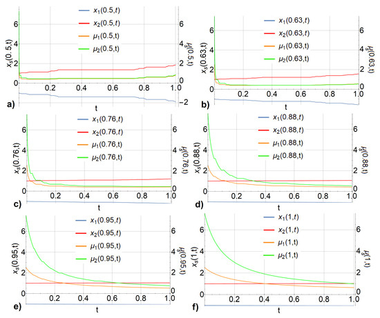
Figure 1.
The zeroth- and first-order moments, ( and , respectively) for two quasiparticles with: (a) , (b) , (c) , (d) , (e) , and (f) for and .
Figure 2 also illustrates that a decrease in the parameter accelerates the evolution of the zeroth-order moment. Additionally, as increases, the total zeroth-order moment approaches the value obtained from the ordinary (first-order) time derivative.
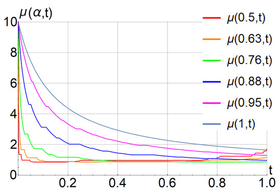
Figure 2.
The zeroth-order moments () for , and 1 and .
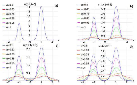
Figure 3 shows the asymptotic solutions () from Equation (20) corresponding to (86) of Equation (17), accurate to for a set of parameters given in (97) and for , , , , , and 1. The solutions are presented at (a) t = 0, (b) t = 0.3, (c) t = 0.6, and (d) t = 1 over the Cantor (set , where ). During the evolution, the asymmetric initial condition (, as shown in Figure 3) evolves toward a symmetric form. As decreases, the evolution of the asymptotic solutions accelerates. In Figure 3, one can observe how the processes of diffusion and growth of the total zeroth-order moment (Figure 2) destroy the dynamics of quasiparticles for . In this case, two local peaks merge in a Gaussian-like function, as shown in panel (d) of Figure 3.
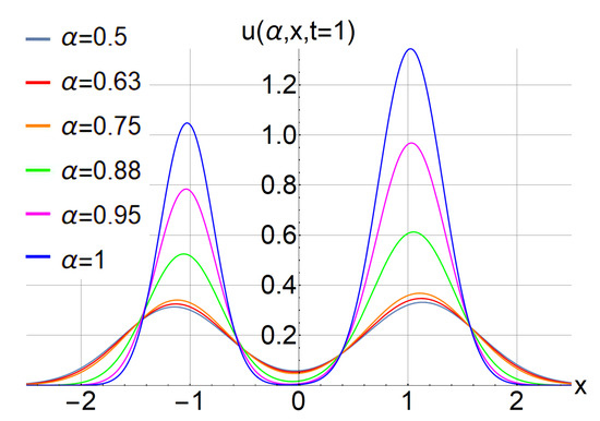
For further investigation, Figure 4 shows asymptotic solutions () (20) constructed on a seventh-generation prefractal with an analogous partition () and parameters (97) at . Comparing these solutions with those for the fifth-generation prefractal in Figure 4, it can be observed that the acceleration in the evolution rate of the asymptotic solutions as decreases diminishes with increasing prefractal generation.
9. Conclusions
In this paper, we extend the methodology proposed in [24] for the construction of asymptotic solutions within the weak diffusion approximation to the nonlocal generalized Fisher–KPP Equation (17). This equation incorporates a fractal time derivative of non-integer order , where . The fractal time derivative is defined within the framework of calculus [5,6,7], incorporating the concept of the Maslov method as discussed in [22,23].
The constructed asymptotic solutions exhibit a nontrivial geometric structure, as represented in (20). Each solution comprises a finite number of localized distributions (quasiparticles), with each quasiparticle concentrated within a distinct spatial neighborhood that defines its coordinates.
The example presented in Section 8 illustrates the impact of fractality on physical diffusion processes in population dynamics through a solution comprising two quasiparticles. Each quasiparticle initially follows a Gaussian density distribution within the framework of the Fisher–KPP model (17). The primary objective of this analysis is to examine how the characteristics of these quasiparticles depend on the parameter of the fractal time derivative (). The graphs in Figure 1, Figure 2 and Figure 3 reveal that diffusion governed by the fractal time derivative () with progresses more rapidly than diffusion described by the standard first-order derivative (). This acceleration arises from the nature of the underlying time intervals: while ordinary diffusion () evolves continuously over time, fractal diffusion () proceeds discontinuously, with events occurring at discrete points within a fractal Cantor-like time set (F). However, we note that as the prefractal order increases, the enhancement in the diffusion rate diminishes (Figure 4). This observation aligns with the conceptual understanding of fractal time intervals, since higher-order prefractals contain an increased number of discrete points, resulting in reduced jump magnitudes during diffusion.
The Einstein–Ehrenfest fractal dynamical system (49)–(51)) plays a crucial role in constructing asymptotic solutions for Equation (21). This system governs the moments (27) of the solutions sought for the system (21) that describes quasiparticles and is formulated within function classes of in the form of (19). The FlEES serves as an analog of the equations of fractal classical mechanics for a system of quasiparticles corresponding to the solution (20) of Equation (17). The interaction between quasiparticles is determined by the structure of Equation (17).
The mathematical properties of the FlEES are of significant interest in the theory of fractal differential equations, as this system emerges in physical and biological models that describe real-world systems with complex structural properties. Furthermore, the formalism developed here for the construction of asymptotic solutions to fractal Equation (17) can be naturally extended to its multidimensional case and applied to other nonlocal generalizations of nonlinear reaction–diffusion dynamics, as demonstrated in studies such as [34,35,36], among others. However, since the asymptotic solutions are constructed within the class of functions defined by Equations (18) and (19), which comprises spatially localized functions, the asymptotics do not work well when the solutions lose their localization properties. This imposes limitations on the temporal scale where the asymptotics are effective. In the model example presented in Section 8, the kernel function () in Equation (17) was chosen to be Gaussian (85) for the sake of simplicity. More generally, the proposed approach is applicable to any smooth function () that grows no faster than a polynomial as , .
Note that for the analysis of dynamical systems of the FlEES type, as well as systems of the AFlLE type (described by Equations (57) and (58)), it appears promising to employ various ideas and approaches from the symmetry analysis of integer-order partial differential equations (e.g., [37,38]), methods of integral transformations (e.g., [39]), various types of approximations (e.g., [29]), and other approaches.
The results presented here provide a foundation for the development of approximate methods for the nonlocal Fisher–KPP equation with fractal spatial partial derivatives, a topic of particular interest in both the theory of fractal equations and their applications in biology and physics.
Author Contributions
Conceptualization, A.V.S. and S.A.S.; methodology, A.V.S. and S.A.S.; software, S.A.S.; validation, A.V.S. and S.A.S.; formal analysis, A.V.S. and S.A.S.; investigation, A.V.S. and S.A.S.; writing—original draft preparation, A.V.S. and S.A.S.; writing—review and editing, A.V.S. and S.A.S.; visualization, S.A.S.; supervision, A.V.S.; project administration, A.V.S. All authors have read and agreed to the published version of the manuscript.
Funding
This research received no external funding.
Data Availability Statement
Data are contained within the article.
Conflicts of Interest
The authors declare no conflicts of interest.
References
- Murray, J.D. Mathematical Biology. I. An Introduction; Springer: New York, NY, USA, 2002. [Google Scholar] [CrossRef]
- dos Santos, M.A.F. Analytic approaches of the anomalous diffusion: A review. Chaos Solitons Fractals 2019, 124, 86–96. [Google Scholar] [CrossRef]
- Ionescu, C.; Lopes, A.; Copot, D.; Machado, J.A.T.; Bates, J.H.T. The role of fractional calculus in modelling biological phenomena: A review. Commun. Nonlin. Sci. Numer. Simul. 2017, 51, 141–159. [Google Scholar] [CrossRef]
- Hafez, M.; Alshowaikh, F.; Wan Niu Voon, B.; Alkhazaleh, S.; Al-Faiz, H. Review on recent advances in fractional differentiation and its applications. Progr. Fract. Differ. Appl. 2025, 11, 245–261. [Google Scholar] [CrossRef]
- Parvate, A.; Gangal, A.D. Calculus on fractal subsets of real line—I: Formulation. Fractals 2009, 17, 53–81. [Google Scholar] [CrossRef]
- Parvate, A.; Gangal, A.D. Calculus on fractal subsets of real line—II: Conjugacy with ordinary calculus. Fractals 2011, 19, 271–290. [Google Scholar] [CrossRef]
- Parvate, A.; Satin, S.; Gangal, A.D. Calculus on fractal curves in Rn. Fractals 2011, 19, 15–27. [Google Scholar] [CrossRef]
- Golmankhaneh, A.K.; Tunç, C.; Nia, S.M.; Golmankhaneh, A.K. A review on local and non-local fractal calculus. Num. Com. Meth. Sci. Eng. 2019, 1, 19–31. [Google Scholar]
- Golmankhaneh, A.K. A review on application of the local fractal calculus. Num. Com. Meth. Sci. Eng. 2019, 1, 57–66. [Google Scholar]
- Deppman, A.; Megias, E.; Pasechnik, R. Fractal derivatives, fractional derivatives and q-deformed calculus. Entropy 2023, 25, 1008. [Google Scholar] [CrossRef]
- Golmankhaneh, A.K. Fractal Calculus and Its Applications. Fα-Calculus; World Scientific: Singapore, 2022; p. 328. [Google Scholar] [CrossRef]
- Fisher, R.A. The wave of advance of advantageous genes. Annu. Eugen. 1937, 7, 255–369. [Google Scholar] [CrossRef]
- Kolmogorov, A.N.; Petrovskii, I.; Piskunov, N. A study of the diffusion equation with increase of substance, and its application to a biological problem. Bull. Univ. Moscow Ser. Int. A 1937, 1, 1–26. [Google Scholar]
- Banerjee, M.; Kuznetsov, M.; Udovenko, O.; Volpert, V. Nonlocal Reaction-Diffusion Equations in Biomedical Applications. Acta Biotheor. 2022, 70, 12. [Google Scholar] [CrossRef]
- Paulau, P.V.; Gomila, D.; Lopez, C.; Hernandez-Garcia, E. Self-localized states in species competition. Phys. Rev. E 2014, 89, 032724. [Google Scholar] [CrossRef] [PubMed]
- Sequeira, T.F.; Lima, P.M. Numerical simulations of one- and two-dimensional stochastic neural field equations with delay. J. Comput. Neurosci. 2022, 50, 299–311. [Google Scholar] [CrossRef]
- Trifonov, A.Y.; Shapovalov, A.V. The one-dimensional Fisher–Kolmogorov equation with a nonlocal nonlinearity in a semiclassical approximation. Russ. Phys. J. 2009, 52, 899–911. [Google Scholar] [CrossRef]
- Shapovalov, A.V.; Trifonov, A.Y. An application of the Maslov complex germ method to the one-dimensional nonlocal Fisher–KPP equation. Int. J. Geom. Methods Mod. Phys. (IJGMMP) 2018, 15, 1850102. [Google Scholar] [CrossRef]
- Shapovalov, A.V.; Trifonov, A.Y. Approximate solutions and symmetry of a two-component nonlocal reaction-diffusion population model of the Fisher–KPP type. Symmetry 2019, 11, 366. [Google Scholar] [CrossRef]
- Siniukov, S.A.; Trifonov, A.Y.; Shapovalov, A.V. Examples of asymptotic solutions obtained by the complex germ method for the one-dimensional nonlocal Fisher–Kolmogorov–Petrovskii–Piskunov equation. Russ. Phys. J. 2021, 64, 1542–1552. [Google Scholar] [CrossRef]
- Kulagin, A.E.; Shapovalov, A.V. Quasiparticles for the one-dimensional nonlocal Fisher-Kolmogorov-Petrovskii-Piskunov equation. Physica Scripta 2024, 99, 045228. [Google Scholar] [CrossRef]
- Maslov, V.P. The Complex WKB Method for Nonlinear Equations. I. Linear Theory; Birkhauser Verlag: Basel, Switzerland, 1994. [Google Scholar] [CrossRef]
- Belov, V.V.; Dobrokhotov, S.Y. Semiclassical Maslov asymptotics with complex phases. I. General approach. Theor. Math. Phys. 1992, 92, 843–868. [Google Scholar] [CrossRef]
- Shapovalov, A.V.; Siniukov, S.A. Fractal dynamics of solution moments for the KPP–Fisher equation. Russ. Phys. J. 2024, 67, 1827–1837. [Google Scholar] [CrossRef]
- Kolwankar, K.M.; Gangal, A.D. Local fractional Fokker–Planck equation. Phys. Rev. Lett. 1998, 80, 214–217. [Google Scholar] [CrossRef]
- Barlow, M.T. Diffusion on Fractals; Lecture Notes in Mathematics; Springer: Berlin/Heidelberg, Germany, 1998; Volume 1690, pp. 1–121. [Google Scholar] [CrossRef]
- Yang, X.-J.; Zhang, Z.-Z.; Machado, J.A.T.; Baleanu, D. On local fractional operators view of computational complexity. Diffusion and relaxation defined on Cantor sets. Therm. Sci. 2016, 20, 755–767. [Google Scholar] [CrossRef]
- Ishii, H. Propagating front solutions in a time-fractional Fisher-KPP equation. Discret. Contin. Dyn. Syst.-B 2024, 30, 2460–2482. [Google Scholar] [CrossRef]
- Awonusika, R.O. Approximate analytical solution of a class of highly nonlinear time-fractional-order partial differential equations. Partial. Differ. Equ. Appl. Math. 2025, 13, 101090. [Google Scholar] [CrossRef]
- Golmankhaneh, A.K.; Fernandez, A.A.; Golmankhaneh, A.K.; Baleanu, D. Diffusion on middle-ζ Cantor sets. Entropy 2018, 20, 504. [Google Scholar] [CrossRef]
- Shapovalov, A.V.; Brons, R. Invariance properties of the one-dimensional diffusion equation with a fractal time derivative. Russ. Phys. J. 2021, 64, 704–716. [Google Scholar] [CrossRef]
- Ashrafi, S.; Golmankhaneh, A.K. Dimension of quantum mechanical path, chain rule, and extension of Landau’s energy straggling method using Fα-calculus. Turk. J. Phys. 2018, 42, 104–115. [Google Scholar] [CrossRef]
- Bagrov, V.G.; Belov, V.V.; Trifonov, A.Y. Semiclassical trajectory-coherent approximation in quantum mechanics: I. High order corrections to multidimensional time-dependent equations of Schrödinger type. Ann. Phys. 1996, 246, 231–280. [Google Scholar] [CrossRef]
- Bessonov, N.; Bocharov, G.; Meyerhans, A.; Popov, V.; Volpert, V. Nonlocal reaction-diffusion model of viral evolution: Emergence of virus strains. Mathematics 2020, 8, 117. [Google Scholar] [CrossRef]
- Banerjee, M.; Petrovskii, S.V.; Volpert, V. Nonlocal reaction-riffusion models of heterogeneous wealth distribution. Mathematics 2021, 9, 351. [Google Scholar] [CrossRef]
- Roquejoffre, J.-M. The Dynamics of Front Propagation in Nonlocal Reaction-Diffusion Equations; Springer: Cham, Switzerland, 2024. [Google Scholar] [CrossRef]
- Obukhov, V. Algebra of symmetry operators for Klein-Gordon-Fock equation. Symmetry 2021, 13, 727. [Google Scholar] [CrossRef]
- Obukhov, V. Algebras of integrals of motion for the Hamilton–Jacobi and Klein–Gordon–Fock equations in spacetime with four-parameter groups of motions in the presence of an external electromagnetic field. J. Math. Phys. 2022, 63, 023505. [Google Scholar] [CrossRef]
- Golmankhaneh, A.K.; Şevli, H.; Cattani, C.; Vidović, Z. Fractal Hankel Transform. Fractal Fract. 2025, 9, 135. [Google Scholar] [CrossRef]
Disclaimer/Publisher’s Note: The statements, opinions and data contained in all publications are solely those of the individual author(s) and contributor(s) and not of MDPI and/or the editor(s). MDPI and/or the editor(s) disclaim responsibility for any injury to people or property resulting from any ideas, methods, instructions or products referred to in the content. |
© 2025 by the authors. Licensee MDPI, Basel, Switzerland. This article is an open access article distributed under the terms and conditions of the Creative Commons Attribution (CC BY) license (https://creativecommons.org/licenses/by/4.0/).