An Approximate Analytical View of Fractional Physical Models in the Frame of the Caputo Operator

Abstract

The development of numerical or analytical solutions for fractional mathematical models describing specific phenomena is an important subject in physics, mathematics, and engineering. This paper’s main objective is to investigate the approximation of the fractional order Caudrey–Dodd–Gibbon ($CDG$) nonlinear equation, which appears in the fields of laser optics and plasma physics. The physical issue is modeled using the Caputo derivative. Adomian and homotopy polynomials facilitate the handling of the nonlinear term. The main innovation in this paper is how the recurrence relation, which generates the series solutions after just a few iterations, is handled. We examined the assumed model in fractional form in order to demonstrate and verify the efficacy of the new methods. Moreover, the numerical simulation is used to show how the physical behavior of the suggested method’s solution has been represented in plots and tables for various fractional orders. We provide three problems of each equation to check the validity of the offered schemes. It is discovered that the outcomes derived are close to the accurate result of the problems illustrated. Additionally, we compare our results with the Laplace residual power series method (LRPSM), the natural transform decomposition method (NTDM), and the homotopy analysis shehu transform method (HASTM). From the comparison, our methods have been demonstrated to be more accurate than alternative approaches. The results demonstrate the significant benefit of the established methodologies in achieving both approximate and accurate solutions to the problems. The results show that the technique is extremely methodical, accurate, and very effective for examining the nature of nonlinear differential equations of arbitrary order that have arisen in related scientific fields.

1. Introduction

The past few years have seen a rise in the awareness of fractional calculus (FC) in theoretical physics and scientific applications, as well as an increase in its apparent accessibility. To categorize FC as exclusively teenage research would be completely false. Its strengths in modeling and wide range of applications to real concerns have led to its increasing usage worldwide and sparked the interest of researchers [1]. A few months of talk between Leibniz and L’Hospital led to the creation of this version of calculus, which is a development of ordinary calculus. It is assumed that the discussion of fractional derivatives would continue even in their absence [2]. The most remarkable advancements in engineering and science over the past thirty years have been discovered within the FC framework. The complexity of heterogeneity phenomena has led to the development of the fractional derivative idea. The behavior of complex media with a diffusion process can be modeled by fractional differential operators. It has been a very useful tool, and differential equations of any order can be used to more easily and precisely depict a variety of issues. As opposed to fractional calculus, which examines and analyzes problem behavior based on past data, classical calculus characterizes the essence of the problem by taking into account its current condition. Fractional calculus is thus one of the diverse fields of mathematics that is both effective and current, dealing with real-world issues with ease and achieving results that are truly remarkable. The behavior of issues emerging in biology, chemistry, plasma physics, engineering, mathematical physics, laser optics, etc. can be demonstrated extremely effectively using fractional order derivatives and integrals [3,4,5,6,7,8].

Nonlinear PDEs are essential in order to simulate real-world systems, capture rich dynamics and behaviors, analyze stability, model and understand complicated events, and advance mathematical theory. Compared to linear PDEs, researchers have found that this approach provides a deeper understanding of the behavior of many mathematical and physical systems, including the Schrödinger equation, which governs wave-duality in quantum physics and optics, the Allen–Cahn equation, which governs oil pollution dynamics in oceanography [9], the nonlinear KdV–Burgers equation [10], the nonlinear Kaup–Kupershmidt equation [11], the Zakharov–Kuznetsov equations [12], and the nonlinear Lax’s Korteweg-de Vries equation [13]. Nonlinear PDEs are widely used in the modeling of complex physical, biological, and engineering processes. Many real-world scenarios exhibit nonlinear behavior, and linear partial differential equations (PDEs) provide simplified approximations. In order to properly describe complex systems, nonlinear PDEs must be effective in capturing the nonlinear interactions, feedback processes, and linkages. Nonlinear wave propagation, turbulent fluid flow, pattern creation, and nonlinear reaction-diffusion processes are a few examples. Systems having nonlinear interactions are frequently investigated using nonlinear PDEs to study emergent behavior. Novel phenomena like solitons, shocks, instabilities, and pattern development can arise as a result of nonlinearities. Researchers can learn more about the underlying mechanisms behind the creation of these complicated and interesting behaviors by examining the solutions of nonlinear PDEs [14,15,16,17]. The treatment of PDEs describing nonlinear and evolutionary notions has made the theory of solitary waves more popular recently. Nonlinear phenomena can be seen in a wide range of scientific disciplines, including solid state physics, plasma physics, fluid dynamics, mathematical biology, and chemical kinetics. The diffusion process, convection–advection, dispersive effects, and dissipative effects are the characteristics of nonlinear issues. These issues were handled using a wide range of analytical solution techniques, including the inverse scattering method, the Bäcklund transformation method, Hirota’s bilinear scheme [18,19,20], the Jacobi elliptic method [21], the tanh method [22], the pseudo spectral method [23], Painleve analysis [24], and other techniques.

Unfortunately, due to the laborious work involved, some of these analytical solutions are difficult to use. It can be difficult and important to understand how nonlinear partial differential equations behave in the physical sciences. Despite this, fractional calculus is crucial for the understanding of nonlinear problems. Accurate solutions to FPDEs are crucial in many scientific fields, including applied mathematics. The majority of FPDE issues typically lack closed-form precise solutions, and finding exact solutions is exceedingly challenging. As a result, numerous numerical techniques have been created to solve both linear and nonlinear FPDEs. For example, Oqielat et al. [25] proposed the Laplace residual power series method to solve the general fractional modified KdV system. Yadav and Singh [26] familiarized themselves with the new alternative variational iteration Elzaki transform method time-fractional generalized Burgers–Fisher equation. Aboodh [27] announced the homotopy perturbation transform method for addressing the porous medium equation. Gao et al. [28] presents a semi-analytical solution to the time-fractional Black Scholes equation (TFBSE) using the homotopy analysis fractional Sumudu transform method. Wang et al. [29] presents the q-homotopy analysis transform method for solving (2+1)-dimensional coupled fractional nonlinear Schrödinger equations. Other applications are listed in the literature [30,31,32,33]. As a result, we are inspired by this scenario to investigate the behavior and approximate solution of the Korteweg-de Vries (KdV) equation in a specific situation [34].

In general, the fifth order KdV equation is given below:

$${\mathbf{w}}_{\varrho }(\varkappa ,\varrho )+\eta {\mathbf{w}}_{\varkappa \varkappa \varkappa \varkappa \varkappa }(\varkappa ,\varrho )+a\mathbf{w}(\varkappa ,\varrho ){\mathbf{w}}_{\varkappa \varkappa \varkappa }(\varkappa ,\varrho )+b{\mathbf{w}}_{\varkappa }(\varkappa ,\varrho ){\mathbf{w}}_{\varkappa \varkappa }(\varkappa ,\varrho )+c{\mathbf{w}}^2(\varkappa ,\varrho ){\mathbf{w}}_{\varkappa }(\varkappa ,\varrho )=0$$

(1)

Here $a,b,c$ and $\eta$ are non-zero arbitrary real parameters, and ${\mathbf{w}}_{\varrho }(\varkappa ,\varrho )$ is a variable. Here, we give approximations to solutions for a specific case of this problem when $a=30$, $b=30$, $c=180$, and $\eta$ = 1. The KdV equation can be written for these specific values as

$${\mathbf{w}}_{\varrho }(\varkappa ,\varrho )+{\mathbf{w}}_{\varkappa \varkappa \varkappa \varkappa \varkappa }(\varkappa ,\varrho )+30\mathbf{w}(\varkappa ,\varrho ){\mathbf{w}}_{\varkappa \varkappa \varkappa }(\varkappa ,\varrho )+30{\mathbf{w}}_{\varkappa }(\varkappa ,\varrho ){\mathbf{w}}_{\varkappa \varkappa }(\varkappa ,\varrho )+180{\mathbf{w}}^2(\varkappa ,\varrho ){\mathbf{w}}_{\varkappa }(\varkappa ,\varrho )=0$$

(2)

The $CDG$ equation is represented by Equation (2). Due to the fact that the fractional Caputo derivative [35] describes the memory of the system at earlier historical phases, this derivative of arbitrary order is useful for illustrating innovative real-world phenomena like atmospheric physics, earthquakes, ocean climate, vibration, dynamical systems, and polymers. Thus, the Caputo type of the $CDG$ equation can be represented as

$$\begin{array}{cc}\hfill & D_{\varrho }^{\beta }\mathbf{w}(\varkappa ,\varrho )+{\mathbf{w}}_{\varkappa \varkappa \varkappa \varkappa \varkappa }(\varkappa ,\varrho )+30\mathbf{w}(\varkappa ,\varrho ){\mathbf{w}}_{\varkappa \varkappa \varkappa }(\varkappa ,\varrho )+30{\mathbf{w}}_{\varkappa }(\varkappa ,\varrho ){\mathbf{w}}_{\varkappa \varkappa }(\varkappa ,\varrho )+180{\mathbf{w}}^2(\varkappa ,\varrho ){\mathbf{w}}_{\varkappa }(\varkappa ,\varrho )\hfill \\ \hfill & =0,0<\beta \le 1,\hfill \end{array}$$

(3)

where $D_{\varrho }^{\beta }$ illustrates the non-integer caputo derivative. The basic $CDG$ equation, which was presented by Caudrey, Dodd, and Gibbon [36], is represented by Equation (3) for $\beta =1$. This nonlinear equation’s fractional model was investigated as a theoretical representation of shallow density-stratified fluid internal waves and shallow water surface waves with tiny amplitudes and long wavelengths. It is particularly significant in laser optics and plasma physics. Since significant factors like convergence, divergence, and the effectiveness of solutions in numerical evaluation are equally relevant in the modeling of nonlinear partial differential equations. Hence, a variety of numerical and analytical techniques are offered for solving the nonlinear PDEs in order to yield more achievable and efficient solutions [37,38,39,40]. Numerous scholars have suggested a wide range of solutions to the $CDG$ equation [40,41,42,43,44]. However, each of these approaches has its own problems and restrictions, such as the need for extensive computational effort, extra memory, time, and inconsistent results.

The use of the Yang transform decomposition method (YTDM) and homotopy perturbation transform method (HPTM), which combine the Yang Transform (YT), ADM, and HPM for solving the fractional $CDG$ problem, is the achievement of this work. Adomain polynomials and He’s polynomials are used to decompose the nonlinear terms after the differential equations are transformed into algebraic equations with the aid of the Yang transform. In summary, the fractional Caputo derivative is approximated using the Yang transform method, converting the original FPDE into its corresponding PDE. By applying the homotopy perturbation methodology and the adomian decomposition method to the resulting PDE, the initial FPDE may be solved rapidly and simply. It is a practical and effective mathematical tool for resolving nonlinear equations, primarily yielding a very accurate solution after just one iteration. These novel strategies were put out to minimize the effort and cost of computing. By using the suggested procedures, convergent series solutions were achieved. The given work is organized as follows: Section 2 discusses the Yang transform as well as arbitrary order derivatives in the Caputo sense. The basic concept of the procedures under consideration is covered in Section 3 and Section 4. In Section 5, we offer the existence results of the proposed methods. In Section 6, the proposed methods with the validity of the error bound theorem are applied. The fractional $CDG$ model’s solution is presented in Section 7. In Section 8, we discuss the graphical and numerical behavior of the proposed methods. In Section 9, we conclude with some final comments.

2. Preliminaries

Here, we define the basic notion of fractional derivatives and Yang transform.

Definition 1.

The expression denoting the Riemann fractional integral of the function $\mathit{w}(\varkappa ,\varrho )$ can be represented by

$$\begin{array}{cc}\hfill & I_{\varrho }^{\beta }\left[\mathit{w}(\varkappa ,\varrho )\right]={\displaystyle \frac{1}{\mathrm{\Gamma }\left(\beta \right)}}{\int }_0^{\varrho }{(\varrho -\lambda )}^{\beta -1}\mathit{w}(\varkappa ,\lambda )d\lambda ,\hfill \\ \hfill & and{I}_0^{\beta }\left[\mathit{w}(\varkappa ,\varrho )\right]=\mathit{w}(\varkappa ,\varrho ).\hfill \end{array}$$

(4)

Definition 2.

The Caputo fractional operator is as [45]

$$\begin{array}{cc}\hfill & D_{\varrho }^{\beta }\mathit{w}(\varkappa ,\varrho )={\displaystyle \frac{1}{\mathrm{\Gamma }(k-\beta )}}{\int }_0^{\varrho }{(\varrho -\beta )}^{k-\beta -1}{\mathit{w}}^{\left(k\right)}(\varkappa ,\lambda )d\lambda ,k-1<\beta \le k,k\in N.\hfill \end{array}$$

(5)

Lemma 1.

For $n<\beta \le 1$, $\varrho \ge 0$ and $k\in R$, we have

$$\begin{array}{cc}\hfill & \left(a\right)D_{\varrho }^{\beta }{\varrho }^k={\displaystyle \frac{\mathrm{\Gamma }(k+1)}{\mathrm{\Gamma }(k+1-\beta )}}{\varrho }^{k-\beta }.\hfill \\ \hfill & \left(b\right)D_{\varrho }^{\beta }{I}_{\varrho }^{\beta }\left[\mathit{w}(\varkappa ,\varrho )\right]=\mathit{w}(\varkappa ,\varrho ).\hfill \\ \hfill & \left(c\right)I_{\varrho }^{\beta }{\varrho }^k={\displaystyle \frac{\mathrm{\Gamma }(k+1)}{\mathrm{\Gamma }(k+1+\beta )}}{\varrho }^{k+\beta }.\hfill \\ \hfill & \left(d\right)I_{\varrho }^{\beta }{D}_{\varrho }^{\beta }\left[\mathit{w}(\varkappa ,\varrho )\right]=\mathit{w}(\varkappa ,\varrho )-\sum _{i=0}^{n-1}{\partial }^i\mathit{w}(\varkappa ,0){\displaystyle \frac{{\varrho }^i}{i!}}.\hfill \end{array}$$

Definition 3.

The YT of the given function is [46]

$$Y\left\{\mathit{w}\left(\varrho \right)\right\}=M\left(u\right)={\int }_0^{\infty }{e}^{{\displaystyle \frac{-\varrho }{u}}}\mathit{w}\left(\varrho \right)d\varrho ,\varrho >0,u\in (-{\varrho }_1,{\varrho }_2),$$

(6)

representing inverse YT as

$$Y^{-1}\left\{M\left(u\right)\right\}=\mathit{w}\left(\varrho \right).$$

(7)

Definition 4.

The YT of the given nth order derivative function is [46]

$$Y\left\{{\mathit{w}}^n\left(\varrho \right)\right\}={\displaystyle \frac{M\left(u\right)}{u^n}}-\sum _{k=0}^{n-1}{\displaystyle \frac{{\mathit{w}}^k\left(0\right)}{u^{n-k-1}}},\forall n=1,2,3,\cdots$$

(8)

Definition 5.

The YT of the given function with fractional order derivative is [46]

$$Y\left\{{\mathit{w}}^{\beta }\left(\varrho \right)\right\}={\displaystyle \frac{M\left(u\right)}{u^{\beta }}}-\sum _{k=0}^{n-1}{\displaystyle \frac{{\mathit{w}}^k\left(0\right)}{u^{\beta -(k+1)}}},0<\beta \le n.$$

(9)

3. Construction of HPTM

To illustrate the basic concept of HPTM, we consider the below differential equation:

$$D_{\varrho }^{\beta }\mathbf{w}(\varkappa ,\varrho )={\mathcal{S}}_1\left[\varkappa \right]\mathbf{w}(\varkappa ,\varrho )+{\mathcal{T}}_1\left[\varkappa \right]\mathbf{w}(\varkappa ,\varrho ),1<\beta \le 2,$$

(10)

with the initial conditions

$$\mathbf{w}(\varkappa ,0)=\xi \left(\varkappa \right),{\displaystyle \frac{\partial }{\partial \varrho }}\mathbf{w}(\varkappa ,0)=\zeta \left(\varkappa \right).$$

Here $D_{\varrho }^{\beta }={\displaystyle \frac{{\partial }^{\beta }}{\partial {\varrho }^{\beta }}}$ represented Caputo fractional derivative, ${\mathcal{S}}_1\left[\varkappa \right]$, ${\mathcal{T}}_1\left[\varkappa \right]$ are linear and nonlinear operators.

On operating YT, we obtain

$$Y\left[D_{\varrho }^{\beta }\mathbf{w}(\varkappa ,\varrho )\right]=Y[{\mathcal{S}}_1\left[\varkappa \right]\mathbf{w}(\varkappa ,\varrho )+{\mathcal{T}}_1\left[\varkappa \right]\mathbf{w}(\varkappa ,\varrho )],$$

(11)

$${\displaystyle \frac{1}{u^{\beta }}}\{M\left(u\right)-u\mathbf{w}\left(0\right)-u^2{\mathbf{w}}^{\prime }\left(0\right)\}=Y[{\mathcal{S}}_1\left[\varkappa \right]\mathbf{w}(\varkappa ,\varrho )+{\mathcal{T}}_1\left[\varkappa \right]\mathbf{w}(\varkappa ,\varrho )].$$

(12)

After simplification, we have

$$M\left(\mathbf{w}\right)=u\mathbf{w}\left(0\right)+u^2{\mathbf{w}}^{\prime }\left(0\right)+u^{\beta }Y[{\mathcal{S}}_1\left[\varkappa \right]\mathbf{w}(\varkappa ,\varrho )+{\mathcal{T}}_1\left[\varkappa \right]\mathbf{w}(\varkappa ,\varrho )].$$

(13)

By operating inverse YT, we have

$$\mathbf{w}(\varkappa ,\varrho )=\mathbf{w}\left(0\right)+{\mathbf{w}}^{\prime }\left(0\right)+Y^{-1}\left[u^{\beta }Y[{\mathcal{S}}_1\left[\varkappa \right]\mathbf{w}(\varkappa ,\varrho )+{\mathcal{T}}_1\left[\varkappa \right]\mathbf{w}(\varkappa ,\varrho )]\right].$$

(14)

Now by means of HPM, we obtain

$$\mathbf{w}(\varkappa ,\varrho )=\sum _{k=0}^{\infty }{ϵ}^k{\mathbf{w}}_k(\varkappa ,\varrho ),$$

(15)

with $ϵ\in [0,1]$.

The nonlinear term is stated as

$${\mathcal{T}}_1\left[\varkappa \right]\mathbf{w}(\varkappa ,\varrho )=\sum _{k=0}^{\infty }{ϵ}^k{H}_n\left(\mathbf{w}\right).$$

(16)

Also, $H_k\left(\mathbf{w}\right)$ denotes He’s polynomials and is

$$H_n({\mathbf{w}}_0,{\mathbf{w}}_1,...,{\mathbf{w}}_n)={\displaystyle \frac{1}{\mathrm{\Gamma }(n+1)}}{D}_{ϵ}^k{\left[{\mathcal{T}}_1\left(\sum _{k=0}^{\infty }{ϵ}^i{\mathbf{w}}_i\right)\right]}_{ϵ=0},$$

(17)

where $D_{ϵ}^k={\displaystyle \frac{{\partial }^k}{\partial {ϵ}^k}}.$

By substituting (15) and (16) in (14), we obtain

$$\sum _{k=0}^{\infty }{ϵ}^k{\mathbf{w}}_k(\varkappa ,\varrho )=\mathbf{w}\left(0\right)+{\mathbf{w}}^{\prime }\left(0\right)+ϵ\times \left(Y^{-1}\left[u^{\beta }Y\{{\mathcal{S}}_1\sum _{k=0}^{\infty }{ϵ}^k{\mathbf{w}}_k(\varkappa ,\varrho )+\sum _{k=0}^{\infty }{ϵ}^k{H}_k\left(\mathbf{w}\right)\}\right]\right).$$

(18)

By the comparison of coefficients of $ϵ$ on both sides, we obtain

$$\begin{array}{cc}\hfill & {ϵ}^0:{\mathbf{w}}_0(\varkappa ,\varrho )=\mathbf{w}\left(0\right)+{\mathbf{w}}^{\prime }\left(0\right),\hfill \\ \hfill & {ϵ}^1:{\mathbf{w}}_1(\varkappa ,\varrho )=Y^{-1}\left[u^{\beta }Y({\mathcal{S}}_1\left[\varkappa \right]{\mathbf{w}}_0(\varkappa ,\varrho )+H_0\left(\mathbf{w}\right))\right],\hfill \\ \hfill & {ϵ}^2:{\mathbf{w}}_2(\varkappa ,\varrho )=Y^{-1}\left[u^{\beta }Y({\mathcal{S}}_1\left[\varkappa \right]{\mathbf{w}}_1(\varkappa ,\varrho )+H_1\left(\mathbf{w}\right))\right],\hfill \\ \hfill & .\hfill \\ \hfill & .\hfill \\ \hfill & .\hfill \\ \hfill & {ϵ}^k:{\mathbf{w}}_k(\varkappa ,\varrho )=Y^{-1}\left[u^{\beta }Y({\mathcal{S}}_1\left[\varkappa \right]{\mathbf{w}}_{k-1}(\varkappa ,\varrho )+H_{k-1}\left(\mathbf{w}\right))\right],\hfill \\ \hfill k>0,k\in N.\end{array}$$

(19)

At the end, the approximate solution ${\mathbf{w}}_k(\varkappa ,\varrho )$ is given by

$$\mathbf{w}(\varkappa ,\varrho )=\underset{M\to \infty }{lim}\sum _{k=1}^M{\mathbf{w}}_k(\varkappa ,\varrho ).$$

(20)

4. Construction of YTDM

To illustrate the basic concept of HPTM, we consider the below differential equation:

$$D_{\varrho }^{\beta }\mathbf{w}(\varkappa ,\varrho )={\mathcal{S}}_1(\varkappa ,\varrho )+{\mathcal{T}}_1(\varkappa ,\varrho ),1<\beta \le 2,$$

(21)

with the initial conditions

$$\mathbf{w}(\varkappa ,0)=\xi \left(\varkappa \right),{\displaystyle \frac{\partial }{\partial \varrho }}\mathbf{w}(\varkappa ,0)=\zeta \left(\varkappa \right).$$

Here $D_{\varrho }^{\beta }={\displaystyle \frac{{\partial }^{\beta }}{\partial {\varrho }^{\beta }}}$ represents the Caputo fractional derivative, and ${\mathcal{S}}_1$, ${\mathcal{T}}_1$ are linear and nonlinear operators.

On operating YT, we obtain

$$\begin{array}{cc}\hfill & Y\left[D_{\varrho }^{\beta }\mathbf{w}(\varkappa ,\varrho )\right]=Y[{\mathcal{S}}_1(\varkappa ,\varrho )+{\mathcal{T}}_1(\varkappa ,\varrho )],\hfill \\ \hfill & {\displaystyle \frac{1}{u^{\beta }}}\{M\left(u\right)-u\mathbf{w}\left(0\right)-u^2{\mathbf{w}}^{\prime }\left(0\right)\}=Y[{\mathcal{S}}_1(\varkappa ,\varrho )+{\mathcal{T}}_1(\varkappa ,\varrho )].\hfill \end{array}$$

(22)

After simplification, we have

$$M\left(\mathbf{w}\right)=u\mathbf{w}\left(0\right)+u^2{\mathbf{w}}^{\prime }\left(0\right)+u^{\beta }Y[{\mathcal{S}}_1(\varkappa ,\varrho )+{\mathcal{T}}_1(\varkappa ,\varrho )].$$

(23)

By operating inverse YT, we have

$$\mathbf{w}(\varkappa ,\varrho )=\mathbf{w}\left(0\right)+{\mathbf{w}}^{\prime }\left(0\right)+Y^{-1}[u^{\beta }Y[{\mathcal{S}}_1(\varkappa ,\varrho )+{\mathcal{T}}_1(\varkappa ,\varrho )].$$

(24)

Now by means of YTDM, we obtain

$$\mathbf{w}(\varkappa ,\varrho )=\sum _{m=0}^{\infty }{\mathbf{w}}_m(\varkappa ,\varrho ).$$

(25)

The nonlinear term is stated as

$${\mathcal{T}}_1(\varkappa ,\varrho )=\sum _{m=0}^{\infty }{\mathcal{A}}_m,$$

(26)

with

$${\mathcal{A}}_m={\displaystyle \frac{1}{m!}}{\left[{\displaystyle \frac{{\partial }^m}{\partial {\ell }^m}}\left\{{\mathcal{T}}_1\left(\sum _{k=0}^{\infty }{\ell }^k{\varkappa }_k,\sum _{k=0}^{\infty }{\ell }^k{\varrho }_k\right)\right\}\right]}_{\ell =0}.$$

(27)

By substituting (25) and (26) into (24), we obtain

$$\sum _{m=0}^{\infty }{\mathbf{w}}_m(\varkappa ,\varrho )=\mathbf{w}\left(0\right)+{\mathbf{w}}^{\prime }\left(0\right)+Y^{-1}{u}^{\beta }\left[Y\left\{{\mathcal{S}}_1(\sum _{m=0}^{\infty }{\varkappa }_m,\sum _{m=0}^{\infty }{\varrho }_m)+\sum _{m=0}^{\infty }{\mathcal{A}}_m\right\}\right].$$

(28)

Hence, the analytical solution is then approximated as

$${\mathbf{w}}_0(\varkappa ,\varrho )=\mathbf{w}\left(0\right)+\varrho {\mathbf{w}}^{\prime }\left(0\right),$$

(29)

$${\mathbf{w}}_1(\varkappa ,\varrho )=Y^{-1}\left[u^{\beta }{Y}^{+}\{{\mathcal{S}}_1({\varkappa }_0,{\varrho }_0)+{\mathcal{A}}_0\}\right].$$

Thus, in general for $m\ge 1$, we have

$${\mathbf{w}}_{m+1}(\varkappa ,\varrho )=Y^{-1}\left[u^{\beta }{Y}^{+}\{{\mathcal{S}}_1({\varkappa }_m,{\varrho }_m)+{\mathcal{A}}_m\}\right].$$

5. Convergence Analysis

Here, we illustrated the suggested techniques existence results.

Theorem 1.

Suppose the precise solution of (10) is $\mathrm{\Psi }(\varkappa ,\varrho )$ and let $\mathrm{\Psi }(\varkappa ,\varrho )$, ${\mathrm{\Psi }}_n(\varkappa ,\varrho )\in H$ and $\beta \in (0,1)$, with H illustrates the Hilbert space. The attained solution ${\sum }_{q=0}^{\infty }{\mathrm{\Psi }}_q(\varkappa ,\varrho )$ tends to $\mathrm{\Psi }(\varkappa ,\varrho )$ if ${\mathrm{\Psi }}_q(\varkappa ,\varrho )\le {\mathrm{\Psi }}_{q-1}(\varkappa ,\varrho )\forall q>A$, i.e., for all $\varkappa >0\exists A>0$, such that $\left|\right|{\mathrm{\Psi }}_{q+n}(\varkappa ,\varrho )\left|\right|\le \beta ,\forall q,n\in N.$

Proof. 

Consider a sequence of ${\sum }_{q=0}^{\infty }{\mathrm{\Psi }}_q(\varkappa ,\varrho ).$

$$\begin{array}{cc}\hfill {\mathcal{Z}}_0(\varkappa ,\varrho )=& {\mathrm{\Psi }}_0(\varkappa ,\varrho ),\hfill \\ \hfill {\mathcal{Z}}_1(\varkappa ,\varrho )=& {\mathrm{\Psi }}_0(\varkappa ,\varrho )+{\mathrm{\Psi }}_1(\varkappa ,\varrho ),\hfill \\ \hfill {\mathcal{Z}}_2(\varkappa ,\varrho )=& {\mathrm{\Psi }}_0(\varkappa ,\varrho )+{\mathrm{\Psi }}_1(\varkappa ,\varrho )+{\mathrm{\Psi }}_2(\varkappa ,\varrho ),\hfill \\ \hfill {\mathcal{Z}}_3(\varkappa ,\varrho )=& {\mathrm{\Psi }}_0(\varkappa ,\varrho )+{\mathrm{\Psi }}_1(\varkappa ,\varrho )+{\mathrm{\Psi }}_2(\varkappa ,\varrho )+{\mathrm{\Psi }}_3(\varkappa ,\varrho ),\hfill \\ \hfill & ⋮\hfill \\ \hfill {\mathcal{Z}}_q(\varkappa ,\varrho )=& {\mathrm{\Psi }}_0(\varkappa ,\varrho )+{\mathrm{\Psi }}_1(\varkappa ,\varrho )+{\mathrm{\Psi }}_2(\varkappa ,\varrho )+\cdots +{\mathrm{\Psi }}_q(\varkappa ,\varrho ).\hfill \end{array}$$

(30)

We have to prove that ${\mathcal{Z}}_q(\varkappa ,\varrho )$ forms a “Cauchy sequence” to attain the desired outcome. Assume

$$\begin{array}{cc}\hfill \left|\right|{\mathcal{Z}}_{q+1}(\varkappa ,\varrho )-{\mathcal{Z}}_q(\varkappa ,\varrho )\left|\right|& =\left|\right|{\mathrm{\Psi }}_{q+1}(\varkappa ,\varrho )\left|\right|\le \beta \left|\right|{\mathrm{\Psi }}_q(\varkappa ,\varrho )\left|\right|\le {\beta }^2\left|\right|{\mathrm{\Psi }}_{q-1}(\varkappa ,\varrho )\left|\right|\le {\beta }^3\left|\right|{\mathrm{\Psi }}_{q-2}(\varkappa ,\varrho )\left|\right|\cdots \hfill \\ \hfill & \le {\beta }_{q+1}\left|\right|{\mathrm{\Psi }}_0(\varkappa ,\varrho )\left|\right|.\hfill \end{array}$$

(31)

For $q,n\in N$, we have

$$\begin{array}{cc}\hfill \left|\right|{\mathcal{Z}}_q(\varkappa ,\varrho )-{\mathcal{Z}}_n(\varkappa ,\varrho )\left|\right|=& \left|\right|{\mathrm{\Psi }}_{q+n}(\varkappa ,\varrho )\left|\right|=\left|\right|{\mathcal{Z}}_q(\varkappa ,\varrho )-{\mathcal{Z}}_{q-1}(\varkappa ,\varrho )+({\mathcal{Z}}_{q-1}(\varkappa ,\varrho )-{\mathcal{Z}}_{q-2}(\varkappa ,\varrho ))\hfill \\ \hfill & +({\mathcal{Z}}_{q-2}(\varkappa ,\varrho )-{\mathcal{Z}}_{q-3}(\varkappa ,\varrho ))+\cdots +({\mathcal{Z}}_{n+1}(\varkappa ,\varrho )-{\mathcal{Z}}_n(\varkappa ,\varrho ))\left|\right|\hfill \\ \hfill \le & \left|\right|{\mathcal{Z}}_q(\varkappa ,\varrho )-{\mathcal{Z}}_{q-1}(\varkappa ,\varrho )\left|\right|+\left|\right|({\mathcal{Z}}_{q-1}(\varkappa ,\varrho )-{\mathcal{Z}}_{q-2}(\varkappa ,\varrho ))\left|\right|\hfill \\ \hfill & +\left|\right|({\mathcal{Z}}_{q-2}(\varkappa ,\varrho )-{\mathcal{Z}}_{q-3}(\varkappa ,\varrho ))\left|\right|+\cdots +\left|\right|({\mathcal{Z}}_{n+1}(\varkappa ,\varrho )-{\mathcal{Z}}_n(\varkappa ,\varrho ))\left|\right|\hfill \\ \hfill \le & {\beta }^q\left|\right|{\mathrm{\Psi }}_0(\varkappa ,\varrho )\left|\right|+{\beta }^{q-1}\left|\right|{\mathrm{\Psi }}_0(\varkappa ,\varrho )\left|\right|+\cdots +{\beta }^{q+1}\left|\right|{\mathrm{\Psi }}_0(\varkappa ,\varrho )\left|\right|\hfill \\ \hfill =& \left|\right|{\mathrm{\Psi }}_0(\varkappa ,\varrho )\left|\right|({\beta }^q+{\beta }^{q-1}+{\beta }^{q+1})\hfill \\ \hfill =& \left|\right|{\mathrm{\Psi }}_0(\varkappa ,\varrho )\left|\right|{\displaystyle \frac{1-{\beta }^{q-n}}{1-{\beta }^{q+1}}}{\beta }^{n+1}.\hfill \end{array}$$

(32)

If $0<\beta <1$, and ${\mathrm{\Psi }}_0(\varkappa ,\varrho )$ are bound, then, assuming $\beta =1-\beta /(1-{\beta }_{q-n}){\beta }^{n+1}\left|\right|{\mathrm{\Psi }}_0(\varkappa ,\varrho )\left|\right|$, we obtain

$$\left|\right|{\mathrm{\Psi }}_{q+n}(\varkappa ,\varrho )\left|\right|\le \beta ,\forall q,n\in N.$$

(33)

Hence, ${\left\{{\mathrm{\Psi }}_q(\varkappa ,\varrho )\right\}}_{q=0}^{\infty }$ forms a “Cauchy sequence” in H, which proves that the sequence ${\left\{{\mathrm{\Psi }}_q(\varkappa ,\varrho )\right\}}_{q=0}^{\infty }$ is a convergent sequence in the limit ${lim}_{q\to \infty }{\mathrm{\Psi }}_q(\varkappa ,\varrho )=\mathrm{\Psi }(\varkappa ,\varrho )$ for $\exists \mathrm{\Psi }(\varkappa ,\varrho )\in \mathcal{H}$, which completes the proof. □

Theorem 2.

Assume that ${\sum }_{h=0}^k{\mathrm{\Psi }}_h(\varkappa ,\varrho )$ is finite and $\mathrm{\Psi }(\varkappa ,\varrho )$ reveal the series solution. Considering $\beta >0$ with $\left|\right|{\mathrm{\Psi }}_{h+1}(\varkappa ,\varrho )\left|\right|\le \left|\right|{\mathrm{\Psi }}_h(\varkappa ,\varrho )\left|\right|$, the maximum absolute error is illustrated as

$$\left|\right|\mathrm{\Psi }(\varkappa ,\varrho )-\sum _{h=0}^k{\mathrm{\Psi }}_h(\varkappa ,\varrho )\left|\right|<{\displaystyle \frac{{\beta }^{k+1}}{1-\beta }}\left|\right|{\mathrm{\Psi }}_0(\varkappa ,\varrho )\left|\right|.$$

(34)

Proof. 

Let ${\sum }_{h=0}^k{\mathrm{\Psi }}_h(\varkappa ,\varrho )$ be finite, which indicates that ${\sum }_{h=0}^k{\mathrm{\Psi }}_h(\varkappa ,\varrho )<\infty$.

Assume

$$\begin{array}{cc}\hfill \left|\right|\mathrm{\Psi }(\varkappa ,\varrho )-\sum _{h=0}^k{\mathrm{\Psi }}_h(\varkappa ,\varrho )\left|\right|=& \left|\right|\sum _{h=k+1}^{\infty }{\mathrm{\Psi }}_h(\varkappa ,\varrho )\left|\right|\hfill \\ \hfill \le & \sum _{h=k+1}^{\infty }\left|\right|{\mathrm{\Psi }}_h(\varkappa ,\varrho )\left|\right|\hfill \\ \hfill \le & \sum _{h=k+1}^{\infty }{\beta }^h\left|\right|{\mathrm{\Psi }}_0(\varkappa ,\varrho )\left|\right|\hfill \\ \hfill \le & {\beta }^{k+1}(1+\beta +{\beta }^2+\cdots )\left|\right|{\mathrm{\Psi }}_0(\varkappa ,\varrho )\left|\right|\hfill \\ \hfill \le & {\displaystyle \frac{{\beta }^{k+1}}{1-\beta }}\left|\right|{\mathrm{\Psi }}_0(\varkappa ,\varrho )\left|\right|,\hfill \end{array}$$

(35)

which is proved. □

Theorem 3.

The outcome of (21) is unique at $0<({\varkappa }_1+{\varkappa }_2)\left({\displaystyle \frac{{\varrho }^{\beta }}{\mathrm{\Gamma }(\beta +1)}}\right)<1.$

Proof. 

Suppose $H=\left(C\right[J],||.|\left|\right)$ with the norm $\left|\right|\varphi \left(\varrho \right)\left|\right|={max}_{\varrho \in J}\left|\varphi \left(\varrho \right)\right|$ is a Banach space, ∀ continuous function on J. Let $I:H\to H$ be a non-linear mapping, thus

$${\mathbf{w}}_{l+1}^C={\mathbf{w}}_0^C+Y^{-1}\left[u^{\beta }Y[{\mathcal{S}}_1\left({\mathbf{w}}_l(\varkappa ,\varrho )\right)+{\mathcal{T}}_1\left({\mathbf{w}}_l(\varkappa ,\varrho )\right)]\right],l\ge 0.$$

Suppose that $|{\mathcal{S}}_1\left(\mathbf{w}\right)-{\mathcal{S}}_1\left({\mathbf{w}}^{*}\right)|<{\varkappa }_1|\mathbf{w}-{\mathbf{w}}^{*}|$ and $|{\mathcal{T}}_1\left(\mathbf{w}\right)-{\mathcal{T}}_1\left({\mathbf{w}}^{*}\right)|<{\varkappa }_2|\mathbf{w}-{\mathbf{w}}^{*}|$, where $\mathbf{w}:=\mathbf{w}(\varkappa ,\varrho )$ and ${\mathbf{w}}^{*}:={\mathbf{w}}^{*}(\varkappa ,\varrho )$ are two separate function values and ${\varkappa }_1$, ${\varkappa }_2$ are Lipschitz constants.

$$\begin{array}{cc}\hfill \left|\right|I\mathbf{w}-I{\mathbf{w}}^{*}\left|\right|& \le ma{x}_{t\in J}|Y^{-1}[u^{\beta }Y[{\mathcal{S}}_1\left(\mathbf{w}\right)-{\mathcal{S}}_1\left({\mathbf{w}}^{*}\right)]\hfill \\ \hfill & +u^{\beta }Y[{\mathcal{T}}_1\left(\mathbf{w}\right)-{\mathcal{T}}_1\left({\mathbf{w}}^{*}\right)]\left]\right|\hfill \\ \hfill & \le ma{x}_{\varrho \in J}[{\varkappa }_1{Y}^{-1}[u^{\beta }Y[|\mathbf{w}-{\mathbf{w}}^{*}\left|\right]]\hfill \\ \hfill & +{\varkappa }_2{Y}^{-1}[u^{\beta }Y[|\mathbf{w}-{\mathbf{w}}^{*}\left|\right]\left]\right]\hfill \\ \hfill & \le ma{x}_{t\in J}({\varkappa }_1+{\varkappa }_2)\left[Y^{-1}[u^{\beta }Y|\mathbf{w}-{\mathbf{w}}^{*}\left|\right]\right]\hfill \\ \hfill & \le ({\varkappa }_1+{\varkappa }_2)\left[Y^{-1}[u^{\beta }Y\left|\right|\mathbf{w}-{\mathbf{w}}^{*}\left|\right|]\right]\hfill \\ \hfill & =({\varkappa }_1+{\varkappa }_2)\left({\displaystyle \frac{{\varrho }^{\beta }}{\mathrm{\Gamma }(\beta +1)}}\right)\left|\right|\mathbf{w}-{\mathbf{w}}^{*}\left|\right|\hfill \end{array}$$

(36)

I is contraction as $0<({\varkappa }_1+{\varkappa }_2)\left({\displaystyle \frac{{\varrho }^{\beta }}{\mathrm{\Gamma }(\beta +1)}}\right)<1$. The outcome of (21) is unique in terms of the Banach fixed point theorem. □

Theorem 4.

The outcome of (21) is convergent.

Proof. 

Assume ${\mathbf{w}}_m={\sum }_{r=0}^m{\mathbf{w}}_r(\varkappa ,\varrho )$. To show that ${\mathbf{w}}_m$ is a Cauchy sequence in H. Consider

$$\begin{array}{cc}\hfill \left|\right|{\mathbf{w}}_m-{\mathbf{w}}_n\left|\right|& =ma{x}_{\varrho \in J}|\sum _{r=n+1}^m{\mathbf{w}}_r|,n=1,2,3,\cdots \hfill \\ \hfill & \le ma{x}_{\varrho \in J}\left|Y^{-1}\left[u^{\beta }Y\left[\sum _{r=n+1}^m({\mathcal{S}}_1\left({\mathbf{w}}_{r-1}\right)+{\mathcal{T}}_1\left({\mathbf{w}}_{r-1}\right))\right]\right]\right|\hfill \\ \hfill & =ma{x}_{\varrho \in J}\left|Y^{-1}\left[u^{\beta }Y\left[\sum _{r=n+1}^{m-1}({\mathcal{S}}_1\left({\mathbf{w}}_r\right)+{\mathcal{T}}_1\left({\mathbf{w}}_r\right))\right]\right]\right|\hfill \\ \hfill & \le ma{x}_{\varrho \in J}\left|Y^{-1}\left[u^{\beta }Y\left[({\mathcal{S}}_1\left({\mathbf{w}}_{m-1}\right)-{\mathcal{S}}_1\left({\mathbf{w}}_{n-1}\right)+{\mathcal{T}}_1\left({\mathbf{w}}_{m-1}\right)-{\mathcal{T}}_1\left({\mathbf{w}}_{n-1}\right))\right]\right]\right|\hfill \\ \hfill & \le {\varkappa }_{1}ma{x}_{\varrho \in J}\left|Y^{-1}\left[u^{\beta }Y\left[({\mathcal{S}}_1\left({\mathbf{w}}_{m-1}\right)-{\mathcal{S}}_1\left({\mathbf{w}}_{n-1}\right))\right]\right]\right|\hfill \\ \hfill & +{\varkappa }_{2}ma{x}_{\varrho \in J}\left|Y^{-1}\left[u^{\beta }Y\left[({\mathcal{T}}_1\left({\mathbf{w}}_{m-1}\right)-{\mathcal{T}}_1\left({\mathbf{w}}_{n-1}\right))\right]\right]\right|\hfill \\ \hfill & =({\varkappa }_1+{\varkappa }_2)\left({\displaystyle \frac{{\varrho }^{\beta }}{\mathrm{\Gamma }(\beta +1)}}\right)\left|\right|{\mathbf{w}}_{m-1}-{\mathbf{w}}_{n-1}\left|\right|\hfill \end{array}$$

(37)

Let $m=n+1$. Then

$$\begin{array}{c}\hfill \left|\right|{\mathbf{w}}_{n+1}-{\mathbf{w}}_n\left|\right|\le \varkappa \left|\right|{\mathbf{w}}_n-{\mathbf{w}}_{n-1}\left|\right|\le {\varkappa }^2\left|\right|{\mathbf{w}}_{n-1}{\mathbf{w}}_{n-2}\left|\right|\le \cdots \le {\varkappa }^n\left|\right|{\mathbf{w}}_1-{\mathbf{w}}_0\left|\right|,\end{array}$$

(38)

where $\varkappa =({\varkappa }_1+{\varkappa }_2)\left({\displaystyle \frac{{\varrho }^{\beta }}{\mathrm{\Gamma }(\beta +1)}}\right)$. Similarly, we have

$$\begin{array}{cc}\hfill \left|\right|{\mathbf{w}}_m-{\mathbf{w}}_n\left|\right|& \le \left|\right|{\mathbf{w}}_{n+1}-{\mathbf{w}}_n\left|\right|+\left|\right|{\mathbf{w}}_{n+2}{\mathbf{w}}_{n+1}\left|\right|+\cdots +\left|\right|{\mathbf{w}}_m-{\mathbf{w}}_{m-1}\left|\right|,\hfill \\ \hfill & ({\varkappa }^n+{\varkappa }^{n+1}+\cdots +{\varkappa }^{m-1})\left|\right|{\mathbf{w}}_1-{\mathbf{w}}_0\left|\right|\hfill \\ \hfill & \le {\varkappa }^n\left({\displaystyle \frac{1-{\varkappa }^{m-n}}{1-\varkappa }}\right)\left|\right|{\mathbf{w}}_1\left|\right|.\hfill \end{array}$$

(39)

As $0<\varkappa <1$, we obtain $1-{\varkappa }^{m-n}<1$. Hence,

$$\begin{array}{c}\hfill \left|\right|{\mathbf{w}}_m-{\mathbf{w}}_n\left|\right|\le {\displaystyle \frac{{\varkappa }^n}{1-\varkappa }}ma{x}_{\varrho \in J}\left|\right|{\mathbf{w}}_1\left|\right|.\end{array}$$

(40)

Since $\left|\right|{\mathbf{w}}_1\left|\right|<\infty ,\left|\right|{\mathbf{w}}_m-{\mathbf{w}}_n\left|\right|\to 0$ when $n\to \infty$. Hence, ${\mathbf{w}}_m$ is a Cauchy sequence in H, demonstrating the series ${\mathbf{w}}_m$ is convergent. □

6. Error Estimation

To examine the precision and effectiveness of the suggested approaches, we present error functions in this section. Assuming that $\mathbf{w}\left(\varrho \right)$ is the precise solution and ${\mathbf{w}}_n\left(\varrho \right)$ is the nth-order approximation of $\mathbf{w}\left(\varrho \right)$ that is generated by the suggested methods, the absolute error $\left(E_n\right)$ in the nth-order approximation is as follows:

$$E_n\left(\varrho \right)=|\mathbf{w}\left(\varrho \right)-{\mathbf{w}}_n\left(\varrho \right)|,$$

(41)

and the maximum absolute error $\left(M{E}_n\right)$ is

$$M{E}_n=ma{x}_{\varrho \in [0,1]}|\mathbf{w}\left(\varrho \right)-{\mathbf{w}}_n\left(\varrho \right)|.$$

(42)

The authors of [47,48,49] used well-known theorems and lemmas to discuss the error bound for their numerical approaches. Using the following theorem, we present an upper bound of absolute error for the suggested methods.

Theorem 5.

(Error bound) Suppose $\mathit{w}\left(\varrho \right)\in C^{(n+1)}[0,1]$ and ${\mathit{w}}_n\left(\varrho \right)={\sum }_{i=0}^n{c}_i{\varrho }^i$ illustrate the accurate and nth-order estimated solution of (10) and (21). Then an upper bound of the absolute error is

$$\left|\right|\mathit{w}\left(\varrho \right)-{\mathit{w}}_n{\left(\varrho \right)\left|\right|}_{\infty }\le {\displaystyle \frac{M}{(n+1)!}}+ma{x}_{0\le i\le n}\left|a_i\right|,$$

(43)

where $M=ma{x}_{0\le t\le 1}\left|{\mathit{w}}^{n+1}\left(\varrho \right)\right|,a_i={\sum }_{i=0}^n\left({\displaystyle \frac{{\mathit{w}}^i\left(0\right)}{i!}}-c_i\right)$.

Proof. 

Assume $\mathbf{w}$ is a continuous function on $[0,1]$. Then the upper bound of $\left|\mathbf{w}\right|$ is taken as

$${\left|\right|\mathbf{w}\left|\right|}_{\infty }=\underset{\varrho \in [0,1]}{sup}\left|\mathbf{w}\left(\varrho \right)\right|.$$

(44)

Employing the norm property, we can obtain

$$\left|\right|\mathbf{w}\left(\varrho \right)-{\mathbf{w}}_n{\left(\varrho \right)\left|\right|}_{\infty }\le \left|\right|\mathbf{w}\left(\varrho \right)-{\mathbf{w}}_n^{*}{\left(\varrho \right)\left|\right|}_{\infty }+\left|\right|{\mathbf{w}}_n^{*}\left(\varrho \right)-\mathbf{w}\left(\varrho \right){\left|\right|}_{\infty }$$

(45)

Since $\mathbf{w}\left(\varrho \right)\in C^{(n+1)}[0,1]$, by the Taylor expansion, we obtain

$$\mathbf{w}\left(\varrho \right)={\mathbf{w}}_n^{*}\left(\varrho \right)+{\displaystyle \frac{{\mathbf{w}}^{n+1}\left({\varrho }_0\right)}{(n+1)!}}{\varrho }^{n+1},{\varrho }_0\in (0,1),$$

(46)

with ${\mathbf{w}}_n^{*}\left(\varrho \right)={\sum }_{i=0}^n{\displaystyle \frac{{\mathbf{w}}^i\left(0\right)}{i!}}{\varrho }^i.$

From (46), we can obtain

$$\begin{array}{cc}\hfill & \left|\right|\mathbf{w}\left(\varrho \right)-{\mathbf{w}}_n^{*}{\left(\varrho \right)\left|\right|}_{\infty }=\underset{0\le \varrho \le 1}{max}\left|{\displaystyle \frac{{\mathbf{w}}^{n+1}\left(\varrho \right)}{(n+1)!}}{\varrho }^{n+1}\right|\hfill \\ \hfill & \le {\displaystyle \frac{1}{(n+1)!}}\underset{0\le \varrho \le 1}{max}\left|{\mathbf{w}}^{n+1}\left(\varrho \right)\right|.\hfill \end{array}$$

(47)

Now we find the value of $\left|\right|\mathbf{w}\left(\varrho \right)-{\mathbf{w}}_n^{*}\left(\varrho \right){\left|\right|}_{\infty }$.

Let $A=(a_0,a_1,\cdots ,a_n),T={(t_0,t_1,\cdots ,t_n)}^T$, with $a_i={\displaystyle \frac{{\mathbf{w}}^i\left(0\right)}{i!}}-c_i,i=0,1,\cdots ,n$. Thus,

$$\begin{array}{cc}\hfill & \parallel {\mathbf{w}}_n^{*}\left(\varrho \right)-{\mathbf{w}}_n\left(\varrho \right)\parallel =\parallel {\displaystyle \sum _{i=0}^n}{\displaystyle \frac{{\mathbf{w}}^i\left(0\right)}{i!}}{\varrho }^i-{\displaystyle \sum _{i=0}^n}{c}_i{\varrho }^i\parallel =\parallel {\displaystyle \sum _{i=0}^n}\left({\displaystyle \frac{{\mathbf{w}}^i\left(0\right)}{i!}}-c_i\right){\varrho }^i\parallel \hfill \\ \hfill & {\parallel A\parallel }_{\infty }.{\parallel T\parallel }_{\infty },\hfill \\ \hfill & \parallel {\mathbf{w}}_n^{*}\left(\varrho \right)-{\mathbf{w}}_n{\left(\varrho \right)\parallel =\parallel A\parallel }_{\infty }.{\parallel T\parallel }_{\infty }.\hfill \end{array}$$

(48)

From (45), (47), and (48) we can obtain

$$\begin{array}{cc}\hfill & \parallel \mathbf{w}\left(\varrho \right)-{\mathbf{w}}_n\left(\varrho \right)\parallel \le \le {\displaystyle \frac{1}{(n+1)!}}\underset{0\le \varrho \le 1}{max}|{\mathbf{w}}^{n+1}{\left(\varrho \right)|+\parallel A\parallel }_{\infty }.{\parallel T\parallel }_{\infty },\hfill \\ \hfill & \parallel \mathbf{w}\left(\varrho \right)-{\mathbf{w}}_n\left(\varrho \right)\parallel \le \le {\displaystyle \frac{M}{(n+1)!}}+\underset{0\le i\le n}{max}\left|a_i\right|,\hfill \end{array}$$

(49)

which completes the proof. □

7. Test Examples

7.1. Example

Assume the fractional nonlinear $CDG$ equation as

$$\begin{array}{cc}\hfill & D_{\varrho }^{\beta }\mathbf{w}(\varkappa ,\varrho )+{\mathbf{w}}_{\varkappa \varkappa \varkappa \varkappa \varkappa }(\varkappa ,\varrho )+30\mathbf{w}(\varkappa ,\varrho ){\mathbf{w}}_{\varkappa \varkappa \varkappa }(\varkappa ,\varrho )+30{\mathbf{w}}_{\varkappa }(\varkappa ,\varrho ){\mathbf{w}}_{\varkappa \varkappa }(\varkappa ,\varrho )+180{\mathbf{w}}^2(\varkappa ,\varrho ){\mathbf{w}}_{\varkappa }(\varkappa ,\varrho )\hfill \\ \hfill & =0,0<\beta \le 1,\hfill \end{array}$$

(50)

having the initial guess

$$\mathbf{w}(\varkappa ,0)={\displaystyle \frac{15+\sqrt{105}}{30}}-{tanh}^2\left(\varkappa \right).$$

• Application of HPTM

On operating YT, we obtain

$$\begin{array}{cc}\hfill & Y\left({\displaystyle \frac{{\partial }^{\beta }\mathbf{w}}{\partial {\varrho }^{\beta }}}\right)=Y(-{\mathbf{w}}_{\varkappa \varkappa \varkappa \varkappa \varkappa }(\varkappa ,\varrho )-30\mathbf{w}(\varkappa ,\varrho ){\mathbf{w}}_{\varkappa \varkappa \varkappa }(\varkappa ,\varrho )-30{\mathbf{w}}_{\varkappa }(\varkappa ,\varrho ){\mathbf{w}}_{\varkappa \varkappa }(\varkappa ,\varrho )-180{\mathbf{w}}^2(\varkappa ,\varrho )\hfill \\ \hfill & {\mathbf{w}}_{\varkappa }(\varkappa ,\varrho )).\hfill \end{array}$$

(51)

By the process of simplification,

$$\begin{array}{cc}\hfill & {\displaystyle \frac{1}{u^{\beta }}}\{M\left(u\right)-u\mathbf{w}\left(0\right)\}=Y(-{\mathbf{w}}_{\varkappa \varkappa \varkappa \varkappa \varkappa }(\varkappa ,\varrho )-30\mathbf{w}(\varkappa ,\varrho ){\mathbf{w}}_{\varkappa \varkappa \varkappa }(\varkappa ,\varrho )-30{\mathbf{w}}_{\varkappa }(\varkappa ,\varrho ){\mathbf{w}}_{\varkappa \varkappa }(\varkappa ,\varrho )-180\hfill \\ \hfill & {\mathbf{w}}^2(\varkappa ,\varrho ){\mathbf{w}}_{\varkappa }(\varkappa ,\varrho )),\hfill \\ \hfill & M\left(u\right)=u\mathbf{w}\left(0\right)+u^{\beta }(-{\mathbf{w}}_{\varkappa \varkappa \varkappa \varkappa \varkappa }(\varkappa ,\varrho )-30\mathbf{w}(\varkappa ,\varrho ){\mathbf{w}}_{\varkappa \varkappa \varkappa }(\varkappa ,\varrho )-30{\mathbf{w}}_{\varkappa }(\varkappa ,\varrho ){\mathbf{w}}_{\varkappa \varkappa }(\varkappa ,\varrho )-180\hfill \\ \hfill & {\mathbf{w}}^2(\varkappa ,\varrho ){\mathbf{w}}_{\varkappa }(\varkappa ,\varrho )).\hfill \end{array}$$

(52)

By operating inverse YT, we have

$$\begin{array}{cc}\hfill & \mathbf{w}(\varkappa ,\varrho )=\mathbf{w}\left(0\right)-Y^{-1}\left[u^{\beta }\right\{Y({\mathbf{w}}_{\varkappa \varkappa \varkappa \varkappa \varkappa }(\varkappa ,\varrho )+30\mathbf{w}(\varkappa ,\varrho ){\mathbf{w}}_{\varkappa \varkappa \varkappa }(\varkappa ,\varrho )+30{\mathbf{w}}_{\varkappa }(\varkappa ,\varrho ){\mathbf{w}}_{\varkappa \varkappa }(\varkappa ,\varrho )+180\hfill \\ \hfill & {\mathbf{w}}^2(\varkappa ,\varrho ){\mathbf{w}}_{\varkappa }(\varkappa ,\varrho )\left)\right\}],\hfill \\ \hfill & \mathbf{w}(\varkappa ,\varrho )={\displaystyle \frac{15+\sqrt{105}}{30}}-{tanh}^2\left(\varkappa \right)-Y^{-1}[u^{\beta }\{Y({\mathbf{w}}_{\varkappa \varkappa \varkappa \varkappa \varkappa }(\varkappa ,\varrho )+30\mathbf{w}(\varkappa ,\varrho ){\mathbf{w}}_{\varkappa \varkappa \varkappa }(\varkappa ,\varrho )+30{\mathbf{w}}_{\varkappa }(\varkappa ,\varrho )\hfill \\ \hfill & {\mathbf{w}}_{\varkappa \varkappa }(\varkappa ,\varrho )+180{\mathbf{w}}^2(\varkappa ,\varrho ){\mathbf{w}}_{\varkappa }(\varkappa ,\varrho )\left)\right\}].\hfill \end{array}$$

(53)

Now by means of HPM, we obtain

$$\begin{array}{cc}\hfill & \sum _{k=0}^{\infty }{ϵ}^k{\mathbf{w}}_k(\varkappa ,\varrho )={\displaystyle \frac{15+\sqrt{105}}{30}}-{tanh}^2\left(\varkappa \right)-ϵ\left(Y^{-1}\right[u^{\beta }Y[{\left(\sum _{k=0}^{\infty }{ϵ}^k{\mathbf{w}}_k(\varkappa ,\varrho ))\right)}_{\varkappa \varkappa \varkappa \varkappa \varkappa }+30\left(\sum _{k=0}^{\infty }{ϵ}^k{H}_k\left(\mathbf{w}\right)\right)+\hfill \\ \hfill & 30\left(\sum _{k=0}^{\infty }{ϵ}^k{H}_k\left(\mathbf{w}\right)\right)+180\left(\sum _{k=0}^{\infty }{ϵ}^k{H}_k\left(\mathbf{w}\right)\right)\left]\right]).\hfill \end{array}$$

(54)

By the comparison of coefficients of $ϵ$ on both sides, we obtain

$$\begin{array}{cc}\hfill & {ϵ}^0:{\mathbf{w}}_0(\varkappa ,\varrho )={\displaystyle \frac{15+\sqrt{105}}{30}}-{tanh}^2\left(\varkappa \right),\hfill \\ \hfill & {ϵ}^1:{\mathbf{w}}_1(\varkappa ,\varrho )=4(11-\sqrt{105}){sech}^2\left(\varkappa \right)tanh\left(\varkappa \right){\displaystyle \frac{{\varrho }^{\beta }}{\mathrm{\Gamma }(\beta +1)}}\hfill \\ \hfill & {ϵ}^2:{\mathbf{w}}_2(\varkappa ,\varrho )={\displaystyle \frac{8(-11+\sqrt{105})(2\sqrt{105}{cosh}^2-22{cosh}^2-3\sqrt{105}+33)}{{cosh}^4}}{\displaystyle \frac{{\varrho }^{2\beta }}{\mathrm{\Gamma }(2\beta +1)}}\hfill \\ \hfill & ⋮\hfill \end{array}$$

At the end, the approximate solution $\mathbf{w}(\varkappa ,\varrho )$ is given by

$$\begin{array}{cc}\hfill & \mathbf{w}(\varkappa ,\varrho )={\mathbf{w}}_0(\varkappa ,\varrho )+{\mathbf{w}}_1(\varkappa ,\varrho )+{\mathbf{w}}_2(\varkappa ,\varrho )+\cdots \hfill \\ \hfill & \mathbf{w}(\varkappa ,\varrho )={\displaystyle \frac{15+\sqrt{105}}{30}}-{tanh}^2\left(\varkappa \right)+4(11-\sqrt{105}){sech}^2\left(\varkappa \right)tanh\left(\varkappa \right){\displaystyle \frac{{\varrho }^{\beta }}{\mathrm{\Gamma }(\beta +1)}}+\hfill \\ \hfill & {\displaystyle \frac{8(-11+\sqrt{105})(2\sqrt{105}{cosh}^2-22{cosh}^2-3\sqrt{105}+33)}{{cosh}^4}}{\displaystyle \frac{{\varrho }^{2\beta }}{\mathrm{\Gamma }(2\beta +1)}}+\cdots \hfill \end{array}$$

• Application of YTDM

On operating YT, we obtain

$$\begin{array}{cc}\hfill & Y\left\{{\displaystyle \frac{{\partial }^{\beta }\mathbf{w}}{\partial {\varrho }^{\beta }}}\right\}=Y(-{\mathbf{w}}_{\varkappa \varkappa \varkappa \varkappa \varkappa }(\varkappa ,\varrho )-30\mathbf{w}(\varkappa ,\varrho ){\mathbf{w}}_{\varkappa \varkappa \varkappa }(\varkappa ,\varrho )-30{\mathbf{w}}_{\varkappa }(\varkappa ,\varrho ){\mathbf{w}}_{\varkappa \varkappa }(\varkappa ,\varrho )-180{\mathbf{w}}^2(\varkappa ,\varrho )\hfill \\ \hfill & {\mathbf{w}}_{\varkappa }(\varkappa ,\varrho )).\hfill \end{array}$$

(55)

After simplification, we have

$$\begin{array}{cc}\hfill & {\displaystyle \frac{1}{u^{\beta }}}\{M\left(u\right)-u\mathbf{w}\left(0\right)\}=Y(-{\mathbf{w}}_{\varkappa \varkappa \varkappa \varkappa \varkappa }(\varkappa ,\varrho )-30\mathbf{w}(\varkappa ,\varrho ){\mathbf{w}}_{\varkappa \varkappa \varkappa }(\varkappa ,\varrho )-30{\mathbf{w}}_{\varkappa }(\varkappa ,\varrho ){\mathbf{w}}_{\varkappa \varkappa }(\varkappa ,\varrho )-180\hfill \\ \hfill & {\mathbf{w}}^2(\varkappa ,\varrho ){\mathbf{w}}_{\varkappa }(\varkappa ,\varrho )),\hfill \\ \hfill & M\left(u\right)=u\mathbf{w}\left(0\right)+u^{\beta }Y(-{\mathbf{w}}_{\varkappa \varkappa \varkappa \varkappa \varkappa }(\varkappa ,\varrho )-30\mathbf{w}(\varkappa ,\varrho ){\mathbf{w}}_{\varkappa \varkappa \varkappa }(\varkappa ,\varrho )-30{\mathbf{w}}_{\varkappa }(\varkappa ,\varrho ){\mathbf{w}}_{\varkappa \varkappa }(\varkappa ,\varrho )-180\hfill \\ \hfill & {\mathbf{w}}^2(\varkappa ,\varrho ){\mathbf{w}}_{\varkappa }(\varkappa ,\varrho )).\hfill \end{array}$$

(56)

By operating inverse YT, we have

$$\begin{array}{cc}\hfill & \mathbf{w}(\varkappa ,\varrho )=\mathbf{w}\left(0\right)+Y^{-1}\left[u^{\beta }\right\{Y({\mathbf{w}}_{\varkappa \varkappa \varkappa \varkappa \varkappa }(\varkappa ,\varrho )+30\mathbf{w}(\varkappa ,\varrho ){\mathbf{w}}_{\varkappa \varkappa \varkappa }(\varkappa ,\varrho )+30{\mathbf{w}}_{\varkappa }(\varkappa ,\varrho ){\mathbf{w}}_{\varkappa \varkappa }(\varkappa ,\varrho )+180\hfill \\ \hfill & {\mathbf{w}}^2(\varkappa ,\varrho ){\mathbf{w}}_{\varkappa }(\varkappa ,\varrho )\left)\right\}],\hfill \\ \hfill & \mathbf{w}(\varkappa ,\varrho )={\displaystyle \frac{15+\sqrt{105}}{30}}-{tanh}^2\left(\varkappa \right)-Y^{-1}[u^{\beta }\{Y({\mathbf{w}}_{\varkappa \varkappa \varkappa \varkappa \varkappa }(\varkappa ,\varrho )+30\mathbf{w}(\varkappa ,\varrho ){\mathbf{w}}_{\varkappa \varkappa \varkappa }(\varkappa ,\varrho )+30{\mathbf{w}}_{\varkappa }(\varkappa ,\varrho )\hfill \\ \hfill & {\mathbf{w}}_{\varkappa \varkappa }(\varkappa ,\varrho )+180{\mathbf{w}}^2(\varkappa ,\varrho ){\mathbf{w}}_{\varkappa }(\varkappa ,\varrho )\left)\right\}].\hfill \end{array}$$

(57)

Now by means of YTDM, we obtain

$$\mathbf{w}(\varkappa ,\varrho )=\sum _{m=0}^{\infty }{\mathbf{w}}_m(\varkappa ,\varrho ).$$

(58)

The nonlinear term is stated as $\mathbf{w}(\varkappa ,\varrho ){\mathbf{w}}_{\varkappa \varkappa \varkappa }(\varkappa ,\varrho )={\sum }_{m=0}^{\infty }{\mathcal{A}}_m,{\mathbf{w}}_{\varkappa }(\varkappa ,\varrho ){\mathbf{w}}_{\varkappa \varkappa }(\varkappa ,\varrho )={\sum }_{m=0}^{\infty }{\mathcal{B}}_m,{\mathbf{w}}^2(\varkappa ,\varrho ){\mathbf{w}}_{\varkappa }(\varkappa ,\varrho )={\sum }_{m=0}^{\infty }{\mathcal{C}}_m$. Therefore, we have

$$\begin{array}{cc}\hfill & \sum _{m=0}^{\infty }{\mathbf{w}}_m(\varkappa ,\varrho )=\mathbf{w}(\varkappa ,0)-Y^{-1}\left[u^{\beta }Y\left[{\mathbf{w}}_{\varkappa \varkappa \varkappa \varkappa \varkappa }(\varkappa ,\varrho )+30\left(\sum _{m=0}^{\infty }{\mathcal{A}}_m\right)+30\left(\sum _{m=0}^{\infty }{\mathcal{B}}_m\right)+180\left(\sum _{m=0}^{\infty }{\mathcal{C}}_m\right)\right]\right],\hfill \\ \hfill & \sum _{m=0}^{\infty }{\mathbf{w}}_m(\varkappa ,\varrho )={\displaystyle \frac{15+\sqrt{105}}{30}}-{tanh}^2\left(\varkappa \right)-Y^{-1}\left[u^{\beta }Y\right[{\mathbf{w}}_{\varkappa \varkappa \varkappa \varkappa \varkappa }(\varkappa ,\varrho )+30\left(\sum _{m=0}^{\infty }{\mathcal{A}}_m\right)+30\left(\sum _{m=0}^{\infty }{\mathcal{B}}_m\right)+\hfill \\ \hfill & 180\left(\sum _{m=0}^{\infty }{\mathcal{C}}_m\right)\left]\right].\hfill \end{array}$$

(59)

Hence, the analytical solution is then approximated as

$${\mathbf{w}}_0(\varkappa ,\varrho )={\displaystyle \frac{15+\sqrt{105}}{30}}-{tanh}^2\left(\varkappa \right).$$

On $m=0$,

$${\mathbf{w}}_1(\varkappa ,\varrho )=4(11-\sqrt{105}){sech}^2\left(\varkappa \right)tanh\left(\varkappa \right){\displaystyle \frac{{\varrho }^{\beta }}{\mathrm{\Gamma }(\beta +1)}}.$$

On $m=1$,

$${\mathbf{w}}_2(\varkappa ,\varrho )={\displaystyle \frac{8(-11+\sqrt{105})(2\sqrt{105}{cosh}^2-22{cosh}^2-3\sqrt{105}+33)}{{cosh}^4}}{\displaystyle \frac{{\varrho }^{2\beta }}{\mathrm{\Gamma }(2\beta +1)}}.$$

By continuing the same procedure we can achieve the remaining terms for $(m\ge 3)$ as

$$\mathbf{w}(\varkappa ,\varrho )=\sum _{m=0}^{\infty }{\mathbf{w}}_m(\varkappa ,\varrho )={\mathbf{w}}_0(\varkappa ,\varrho )+{\mathbf{w}}_1(\varkappa ,\varrho )+{\mathbf{w}}_2(\varkappa ,\varrho )+\cdots$$

$$\begin{array}{cc}\hfill & \mathbf{w}(\varkappa ,\varrho )={\displaystyle \frac{15+\sqrt{105}}{30}}-{tanh}^2\left(\varkappa \right)+4(11-\sqrt{105}){sech}^2\left(\varkappa \right)tanh\left(\varkappa \right){\displaystyle \frac{{\varrho }^{\beta }}{\mathrm{\Gamma }(\beta +1)}}+\hfill \\ \hfill & {\displaystyle \frac{8(-11+\sqrt{105})(2\sqrt{105}{cosh}^2-22{cosh}^2-3\sqrt{105}+33)}{{cosh}^4}}{\displaystyle \frac{{\varrho }^{2\beta }}{\mathrm{\Gamma }(2\beta +1)}}+\cdots \hfill \end{array}$$

By choosing $\beta =1$, we have

$$\mathbf{w}(\varkappa ,\varrho )={\displaystyle \frac{15+\sqrt{105}}{30}}-{tanh}^2(\varkappa -2(11-\sqrt{105})\varrho )$$

(60)

7.2. Example

Assume the fractional nonlinear $CDG$ equation as

$$\begin{array}{cc}\hfill & D_{\varrho }^{\beta }\mathbf{w}(\varkappa ,\varrho )+{\mathbf{w}}_{\varkappa \varkappa \varkappa \varkappa \varkappa }(\varkappa ,\varrho )+30\mathbf{w}(\varkappa ,\varrho ){\mathbf{w}}_{\varkappa \varkappa \varkappa }(\varkappa ,\varrho )+30{\mathbf{w}}_{\varkappa }(\varkappa ,\varrho ){\mathbf{w}}_{\varkappa \varkappa }(\varkappa ,\varrho )+180{\mathbf{w}}^2(\varkappa ,\varrho ){\mathbf{w}}_{\varkappa }(\varkappa ,\varrho )\hfill \\ \hfill & =0,\hfill \\ \hfill 0<\beta \le 1,\end{array}$$

(61)

having the initial guess

$$\mathbf{w}(\varkappa ,0)={\displaystyle \frac{1}{4}}{\kappa }^2{sech}^2\left({\displaystyle \frac{1}{2}}\kappa \varkappa +\mathit{c}\right).$$

• Application of HPTM

On operating YT, we obtain

$$\begin{array}{cc}\hfill & Y\left({\displaystyle \frac{{\partial }^{\beta }\mathbf{w}}{\partial {\varrho }^{\beta }}}\right)=Y(-{\mathbf{w}}_{\varkappa \varkappa \varkappa \varkappa \varkappa }(\varkappa ,\varrho )-30\mathbf{w}(\varkappa ,\varrho ){\mathbf{w}}_{\varkappa \varkappa \varkappa }(\varkappa ,\varrho )-30{\mathbf{w}}_{\varkappa }(\varkappa ,\varrho ){\mathbf{w}}_{\varkappa \varkappa }(\varkappa ,\varrho )-180{\mathbf{w}}^2(\varkappa ,\varrho )\hfill \\ \hfill & {\mathbf{w}}_{\varkappa }(\varkappa ,\varrho )).\hfill \end{array}$$

(62)

By the process of simplification,

$$\begin{array}{cc}\hfill & {\displaystyle \frac{1}{u^{\beta }}}\{M\left(u\right)-u\mathbf{w}\left(0\right)\}=Y(-{\mathbf{w}}_{\varkappa \varkappa \varkappa \varkappa \varkappa }(\varkappa ,\varrho )-30\mathbf{w}(\varkappa ,\varrho ){\mathbf{w}}_{\varkappa \varkappa \varkappa }(\varkappa ,\varrho )-30{\mathbf{w}}_{\varkappa }(\varkappa ,\varrho ){\mathbf{w}}_{\varkappa \varkappa }(\varkappa ,\varrho )-180\hfill \\ \hfill & {\mathbf{w}}^2(\varkappa ,\varrho ){\mathbf{w}}_{\varkappa }(\varkappa ,\varrho )),\hfill \\ \hfill & M\left(u\right)=u\mathbf{w}\left(0\right)+u^{\beta }(-{\mathbf{w}}_{\varkappa \varkappa \varkappa \varkappa \varkappa }(\varkappa ,\varrho )-30\mathbf{w}(\varkappa ,\varrho ){\mathbf{w}}_{\varkappa \varkappa \varkappa }(\varkappa ,\varrho )-30{\mathbf{w}}_{\varkappa }(\varkappa ,\varrho ){\mathbf{w}}_{\varkappa \varkappa }(\varkappa ,\varrho )-180\hfill \\ \hfill & {\mathbf{w}}^2(\varkappa ,\varrho ){\mathbf{w}}_{\varkappa }(\varkappa ,\varrho )).\hfill \end{array}$$

(63)

By operating inverse YT, we have

$$\begin{array}{cc}\hfill & \mathbf{w}(\varkappa ,\varrho )=\mathbf{w}\left(0\right)-Y^{-1}\left[u^{\beta }\right\{Y({\mathbf{w}}_{\varkappa \varkappa \varkappa \varkappa \varkappa }(\varkappa ,\varrho )+30\mathbf{w}(\varkappa ,\varrho ){\mathbf{w}}_{\varkappa \varkappa \varkappa }(\varkappa ,\varrho )+30{\mathbf{w}}_{\varkappa }(\varkappa ,\varrho ){\mathbf{w}}_{\varkappa \varkappa }(\varkappa ,\varrho )+180\hfill \\ \hfill & {\mathbf{w}}^2(\varkappa ,\varrho ){\mathbf{w}}_{\varkappa }(\varkappa ,\varrho )\left)\right\}],\hfill \\ \hfill & \mathbf{w}(\varkappa ,\varrho )={\displaystyle \frac{1}{4}}{\kappa }^2{sech}^2\left({\displaystyle \frac{1}{2}}\kappa \varkappa +\mathit{c}\right)-Y^{-1}[u^{\beta }\{Y({\mathbf{w}}_{\varkappa \varkappa \varkappa \varkappa \varkappa }(\varkappa ,\varrho )+30\mathbf{w}(\varkappa ,\varrho ){\mathbf{w}}_{\varkappa \varkappa \varkappa }(\varkappa ,\varrho )+30{\mathbf{w}}_{\varkappa }(\varkappa ,\varrho )\hfill \\ \hfill & {\mathbf{w}}_{\varkappa \varkappa }(\varkappa ,\varrho )+180{\mathbf{w}}^2(\varkappa ,\varrho ){\mathbf{w}}_{\varkappa }(\varkappa ,\varrho )\left)\right\}].\hfill \end{array}$$

(64)

Now by means of HPM, we obtain

$$\begin{array}{cc}\hfill & \sum _{k=0}^{\infty }{ϵ}^k{\mathbf{w}}_k(\varkappa ,\varrho )={\displaystyle \frac{1}{4}}{\kappa }^2{sech}^2\left({\displaystyle \frac{1}{2}}\kappa \varkappa +\mathit{c}\right)-ϵ\left(Y^{-1}\right[u^{\beta }Y[{\left(\sum _{k=0}^{\infty }{ϵ}^k{\mathbf{w}}_k(\varkappa ,\varrho ))\right)}_{\varkappa \varkappa \varkappa \varkappa \varkappa }+30\left(\sum _{k=0}^{\infty }{ϵ}^k{H}_k\left(\mathbf{w}\right)\right)+\hfill \\ \hfill & 30\left(\sum _{k=0}^{\infty }{ϵ}^k{H}_k\left(\mathbf{w}\right)\right)+180\left(\sum _{k=0}^{\infty }{ϵ}^k{H}_k\left(\mathbf{w}\right)\right)\left]\right]).\hfill \end{array}$$

(65)

By the comparison of coefficients of $ϵ$ on both sides, we obtain

$$\begin{array}{cc}\hfill & {ϵ}^0:{\mathbf{w}}_0(\varkappa ,\varrho )={\displaystyle \frac{1}{4}}{\kappa }^2{sech}^2\left({\displaystyle \frac{1}{2}}\kappa \varkappa +\mathit{c}\right),\hfill \\ \hfill & {ϵ}^1:{\mathbf{w}}_1(\varkappa ,\varrho )={\displaystyle \frac{1}{4}}{\displaystyle \frac{sinh\left(\frac{1}{2}\kappa \varkappa +\mathit{c}\right){\kappa }^7}{{cosh}^3\left(\frac{1}{2}\kappa \varkappa +\mathit{c}\right)}}{\displaystyle \frac{{\varrho }^{\beta }}{\mathrm{\Gamma }(\beta +1)}}\hfill \\ \hfill & {ϵ}^2:{\mathbf{w}}_2(\varkappa ,\varrho )={\displaystyle \frac{1}{8}}{\displaystyle \frac{{\kappa }^{12}\left(2{cosh}^2\left(\frac{1}{2}\kappa \varkappa +\mathit{c}\right)-3\right)}{{cosh}^4\left(\frac{1}{2}\kappa \varkappa +\mathit{c}\right)}}{\displaystyle \frac{{\varrho }^{2\beta }}{\mathrm{\Gamma }(2\beta +1)}}\hfill \\ \hfill & ⋮\hfill \end{array}$$

At the end, the approximate solution $\mathbf{w}(\varkappa ,\varrho )$ is given by

$$\begin{array}{cc}\hfill & \mathbf{w}(\varkappa ,\varrho )={\mathbf{w}}_0(\varkappa ,\varrho )+{\mathbf{w}}_1(\varkappa ,\varrho )+{\mathbf{w}}_2(\varkappa ,\varrho )+\cdots \hfill \\ \hfill & \mathbf{w}(\varkappa ,\varrho )={\displaystyle \frac{1}{4}}{\kappa }^2{sech}^2\left({\displaystyle \frac{1}{2}}\kappa \varkappa +\mathit{c}\right)+{\displaystyle \frac{1}{4}}{\displaystyle \frac{sinh\left(\frac{1}{2}\kappa \varkappa +\mathit{c}\right){\kappa }^7}{{cosh}^3\left(\frac{1}{2}\kappa \varkappa +\mathit{c}\right)}}{\displaystyle \frac{{\varrho }^{\beta }}{\mathrm{\Gamma }(\beta +1)}}+\hfill \\ \hfill & {\displaystyle \frac{1}{8}}{\displaystyle \frac{{\kappa }^{12}\left(2{cosh}^2\left(\frac{1}{2}\kappa \varkappa +\mathit{c}\right)-3\right)}{{cosh}^4\left(\frac{1}{2}\kappa \varkappa +\mathit{c}\right)}}{\displaystyle \frac{{\varrho }^{2\beta }}{\mathrm{\Gamma }(2\beta +1)}}+\cdots \hfill \end{array}$$

• Application of YTDM

On operating YT, we obtain

$$\begin{array}{cc}\hfill & Y\left\{{\displaystyle \frac{{\partial }^{\beta }\mathbf{w}}{\partial {\varrho }^{\beta }}}\right\}=Y(-{\mathbf{w}}_{\varkappa \varkappa \varkappa \varkappa \varkappa }(\varkappa ,\varrho )-30\mathbf{w}(\varkappa ,\varrho ){\mathbf{w}}_{\varkappa \varkappa \varkappa }(\varkappa ,\varrho )-30{\mathbf{w}}_{\varkappa }(\varkappa ,\varrho ){\mathbf{w}}_{\varkappa \varkappa }(\varkappa ,\varrho )-180{\mathbf{w}}^2(\varkappa ,\varrho )\hfill \\ \hfill & {\mathbf{w}}_{\varkappa }(\varkappa ,\varrho )).\hfill \end{array}$$

(66)

After simplification, we have

$$\begin{array}{cc}\hfill & {\displaystyle \frac{1}{u^{\beta }}}\{M\left(u\right)-u\mathbf{w}\left(0\right)\}=Y(-{\mathbf{w}}_{\varkappa \varkappa \varkappa \varkappa \varkappa }(\varkappa ,\varrho )-30\mathbf{w}(\varkappa ,\varrho ){\mathbf{w}}_{\varkappa \varkappa \varkappa }(\varkappa ,\varrho )-30{\mathbf{w}}_{\varkappa }(\varkappa ,\varrho ){\mathbf{w}}_{\varkappa \varkappa }(\varkappa ,\varrho )-180\hfill \\ \hfill & {\mathbf{w}}^2(\varkappa ,\varrho ){\mathbf{w}}_{\varkappa }(\varkappa ,\varrho )),\hfill \\ \hfill & M\left(u\right)=u\mathbf{w}\left(0\right)+u^{\beta }Y(-{\mathbf{w}}_{\varkappa \varkappa \varkappa \varkappa \varkappa }(\varkappa ,\varrho )-30\mathbf{w}(\varkappa ,\varrho ){\mathbf{w}}_{\varkappa \varkappa \varkappa }(\varkappa ,\varrho )-30{\mathbf{w}}_{\varkappa }(\varkappa ,\varrho ){\mathbf{w}}_{\varkappa \varkappa }(\varkappa ,\varrho )-180\hfill \\ \hfill & {\mathbf{w}}^2(\varkappa ,\varrho ){\mathbf{w}}_{\varkappa }(\varkappa ,\varrho )).\hfill \end{array}$$

(67)

By operating inverse YT, we have

$$\begin{array}{cc}\hfill & \mathbf{w}(\varkappa ,\varrho )=\mathbf{w}\left(0\right)+Y^{-1}\left[u^{\beta }\right\{Y({\mathbf{w}}_{\varkappa \varkappa \varkappa \varkappa \varkappa }(\varkappa ,\varrho )+30\mathbf{w}(\varkappa ,\varrho ){\mathbf{w}}_{\varkappa \varkappa \varkappa }(\varkappa ,\varrho )+30{\mathbf{w}}_{\varkappa }(\varkappa ,\varrho ){\mathbf{w}}_{\varkappa \varkappa }(\varkappa ,\varrho )+180\hfill \\ \hfill & {\mathbf{w}}^2(\varkappa ,\varrho ){\mathbf{w}}_{\varkappa }(\varkappa ,\varrho )\left)\right\}],\hfill \\ \hfill & \mathbf{w}(\varkappa ,\varrho )={\displaystyle \frac{1}{4}}{\kappa }^2{sech}^2\left({\displaystyle \frac{1}{2}}\kappa \varkappa +\mathit{c}\right)-Y^{-1}[u^{\beta }\{Y({\mathbf{w}}_{\varkappa \varkappa \varkappa \varkappa \varkappa }(\varkappa ,\varrho )+30\mathbf{w}(\varkappa ,\varrho ){\mathbf{w}}_{\varkappa \varkappa \varkappa }(\varkappa ,\varrho )+30{\mathbf{w}}_{\varkappa }(\varkappa ,\varrho )\hfill \\ \hfill & {\mathbf{w}}_{\varkappa \varkappa }(\varkappa ,\varrho )+180{\mathbf{w}}^2(\varkappa ,\varrho ){\mathbf{w}}_{\varkappa }(\varkappa ,\varrho )\left)\right\}].\hfill \end{array}$$

(68)

Now by means of YTDM, we obtain

$$\mathbf{w}(\varkappa ,\varrho )=\sum _{m=0}^{\infty }{\mathbf{w}}_m(\varkappa ,\varrho ).$$

(69)

The nonlinear term is stated as $\mathbf{w}(\varkappa ,\varrho ){\mathbf{w}}_{\varkappa \varkappa \varkappa }(\varkappa ,\varrho )={\sum }_{m=0}^{\infty }{\mathcal{A}}_m,{\mathbf{w}}_{\varkappa }(\varkappa ,\varrho ){\mathbf{w}}_{\varkappa \varkappa }(\varkappa ,\varrho )={\sum }_{m=0}^{\infty }{\mathcal{B}}_m,{\mathbf{w}}^2(\varkappa ,\varrho ){\mathbf{w}}_{\varkappa }(\varkappa ,\varrho )={\sum }_{m=0}^{\infty }{\mathcal{C}}_m$. Therefore, we have

$$\begin{array}{cc}\hfill & \sum _{m=0}^{\infty }{\mathbf{w}}_m(\varkappa ,\varrho )=\mathbf{w}(\varkappa ,0)-Y^{-1}\left[u^{\beta }Y\left[{\mathbf{w}}_{\varkappa \varkappa \varkappa \varkappa \varkappa }(\varkappa ,\varrho )+30\left(\sum _{m=0}^{\infty }{\mathcal{A}}_m\right)+30\left(\sum _{m=0}^{\infty }{\mathcal{B}}_m\right)+180\left(\sum _{m=0}^{\infty }{\mathcal{C}}_m\right)\right]\right],\hfill \\ \hfill & \sum _{m=0}^{\infty }{\mathbf{w}}_m(\varkappa ,\varrho )={\displaystyle \frac{1}{4}}{\kappa }^2{sech}^2\left({\displaystyle \frac{1}{2}}\kappa \varkappa +\mathit{c}\right)-Y^{-1}\left[u^{\beta }Y\right[{\mathbf{w}}_{\varkappa \varkappa \varkappa \varkappa \varkappa }(\varkappa ,\varrho )+30\left(\sum _{m=0}^{\infty }{\mathcal{A}}_m\right)+30\left(\sum _{m=0}^{\infty }{\mathcal{B}}_m\right)+\hfill \\ \hfill & 180\left(\sum _{m=0}^{\infty }{\mathcal{C}}_m\right)\left]\right].\hfill \end{array}$$

(70)

Hence, the analytical solution is then approximated as

$${\mathbf{w}}_0(\varkappa ,\varrho )={\displaystyle \frac{1}{4}}{\kappa }^2{sech}^2\left({\displaystyle \frac{1}{2}}\kappa \varkappa +\mathit{c}\right).$$

On $m=0$,

$${\mathbf{w}}_1(\varkappa ,\varrho )={\displaystyle \frac{1}{4}}{\displaystyle \frac{sinh\left(\frac{1}{2}\kappa \varkappa +\mathit{c}\right){\kappa }^7}{{cosh}^3\left(\frac{1}{2}\kappa \varkappa +\mathit{c}\right)}}{\displaystyle \frac{{\varrho }^{\beta }}{\mathrm{\Gamma }(\beta +1)}}.$$

On $m=1$,

$${\mathbf{w}}_2(\varkappa ,\varrho )={\displaystyle \frac{1}{8}}{\displaystyle \frac{{\kappa }^{12}\left(2{cosh}^2\left(\frac{1}{2}\kappa \varkappa +\mathit{c}\right)-3\right)}{{cosh}^4\left(\frac{1}{2}\kappa \varkappa +\mathit{c}\right)}}{\displaystyle \frac{{\varrho }^{2\beta }}{\mathrm{\Gamma }(2\beta +1)}}.$$

By continuing the same procedure we can achieve the remaining terms for $(m\ge 3)$ as

$$\mathbf{w}(\varkappa ,\varrho )=\sum _{m=0}^{\infty }{\mathbf{w}}_m(\varkappa ,\varrho )={\mathbf{w}}_0(\varkappa ,\varrho )+{\mathbf{w}}_1(\varkappa ,\varrho )+{\mathbf{w}}_2(\varkappa ,\varrho )+\cdots$$

$$\begin{array}{cc}\hfill & \mathbf{w}(\varkappa ,\varrho )={\displaystyle \frac{1}{4}}{\kappa }^2{sech}^2\left({\displaystyle \frac{1}{2}}\kappa \varkappa +\mathit{c}\right)+{\displaystyle \frac{1}{4}}{\displaystyle \frac{sinh\left(\frac{1}{2}\kappa \varkappa +\mathit{c}\right){\kappa }^7}{{cosh}^3\left(\frac{1}{2}\kappa \varkappa +\mathit{c}\right)}}{\displaystyle \frac{{\varrho }^{\beta }}{\mathrm{\Gamma }(\beta +1)}}+\hfill \\ \hfill & {\displaystyle \frac{1}{8}}{\displaystyle \frac{{\kappa }^{12}\left(2{cosh}^2\left(\frac{1}{2}\kappa \varkappa +\mathit{c}\right)-3\right)}{{cosh}^4\left(\frac{1}{2}\kappa \varkappa +\mathit{c}\right)}}{\displaystyle \frac{{\varrho }^{2\beta }}{\mathrm{\Gamma }(2\beta +1)}}+\cdots \hfill \end{array}$$

By choosing $\beta =1$, we have

$$\mathbf{w}(\varkappa ,\varrho )={\displaystyle \frac{1}{4}}{\kappa }^2{sech}^2\left({\displaystyle \frac{1}{2}}\kappa \varkappa -{\displaystyle \frac{1}{2}}{\kappa }^5\varrho +\mathit{c}\right)$$

(71)

7.3. Example

Assume the fractional nonlinear $CDG$ equation as

$$\begin{array}{cc}\hfill & D_{\varrho }^{\beta }\mathbf{w}(\varkappa ,\varrho )+{\mathbf{w}}_{\varkappa \varkappa \varkappa \varkappa \varkappa }(\varkappa ,\varrho )+30\mathbf{w}(\varkappa ,\varrho ){\mathbf{w}}_{\varkappa \varkappa \varkappa }(\varkappa ,\varrho )+30{\mathbf{w}}_{\varkappa }(\varkappa ,\varrho ){\mathbf{w}}_{\varkappa \varkappa }(\varkappa ,\varrho )+180{\mathbf{w}}^2(\varkappa ,\varrho ){\mathbf{w}}_{\varkappa }(\varkappa ,\varrho )\hfill \\ \hfill & =0,0<\beta \le 1,\hfill \end{array}$$

(72)

having initial guess

$$\mathbf{w}(\varkappa ,0)={\mu }^2{sech}^2\left(\mu \varkappa \right).$$

• Application of HPTM

On operating YT, we obtain

$$\begin{array}{cc}\hfill & Y\left({\displaystyle \frac{{\partial }^{\beta }\mathbf{w}}{\partial {\varrho }^{\beta }}}\right)=Y(-{\mathbf{w}}_{\varkappa \varkappa \varkappa \varkappa \varkappa }(\varkappa ,\varrho )-30\mathbf{w}(\varkappa ,\varrho ){\mathbf{w}}_{\varkappa \varkappa \varkappa }(\varkappa ,\varrho )-30{\mathbf{w}}_{\varkappa }(\varkappa ,\varrho ){\mathbf{w}}_{\varkappa \varkappa }(\varkappa ,\varrho )-180{\mathbf{w}}^2(\varkappa ,\varrho )\hfill \\ \hfill & {\mathbf{w}}_{\varkappa }(\varkappa ,\varrho )).\hfill \end{array}$$

(73)

By the process of simplification,

$$\begin{array}{cc}\hfill & {\displaystyle \frac{1}{u^{\beta }}}\{M\left(u\right)-u\mathbf{w}\left(0\right)\}=Y(-{\mathbf{w}}_{\varkappa \varkappa \varkappa \varkappa \varkappa }(\varkappa ,\varrho )-30\mathbf{w}(\varkappa ,\varrho ){\mathbf{w}}_{\varkappa \varkappa \varkappa }(\varkappa ,\varrho )-30{\mathbf{w}}_{\varkappa }(\varkappa ,\varrho ){\mathbf{w}}_{\varkappa \varkappa }(\varkappa ,\varrho )-180\hfill \\ \hfill & {\mathbf{w}}^2(\varkappa ,\varrho ){\mathbf{w}}_{\varkappa }(\varkappa ,\varrho )),\hfill \\ \hfill & M\left(u\right)=u\mathbf{w}\left(0\right)+u^{\beta }(-{\mathbf{w}}_{\varkappa \varkappa \varkappa \varkappa \varkappa }(\varkappa ,\varrho )-30\mathbf{w}(\varkappa ,\varrho ){\mathbf{w}}_{\varkappa \varkappa \varkappa }(\varkappa ,\varrho )-30{\mathbf{w}}_{\varkappa }(\varkappa ,\varrho ){\mathbf{w}}_{\varkappa \varkappa }(\varkappa ,\varrho )-180\hfill \\ \hfill & {\mathbf{w}}^2(\varkappa ,\varrho ){\mathbf{w}}_{\varkappa }(\varkappa ,\varrho )).\hfill \end{array}$$

(74)

By operating inverse YT, we have

$$\begin{array}{cc}\hfill & \mathbf{w}(\varkappa ,\varrho )=\mathbf{w}\left(0\right)-Y^{-1}\left[u^{\beta }\right\{Y({\mathbf{w}}_{\varkappa \varkappa \varkappa \varkappa \varkappa }(\varkappa ,\varrho )+30\mathbf{w}(\varkappa ,\varrho ){\mathbf{w}}_{\varkappa \varkappa \varkappa }(\varkappa ,\varrho )+30{\mathbf{w}}_{\varkappa }(\varkappa ,\varrho ){\mathbf{w}}_{\varkappa \varkappa }(\varkappa ,\varrho )+180\hfill \\ \hfill & {\mathbf{w}}^2(\varkappa ,\varrho ){\mathbf{w}}_{\varkappa }(\varkappa ,\varrho )\left)\right\}],\hfill \\ \hfill & \mathbf{w}(\varkappa ,\varrho )={\mu }^2{sech}^2\left(\mu \varkappa \right)-Y^{-1}\left[u^{\beta }\right\{Y({\mathbf{w}}_{\varkappa \varkappa \varkappa \varkappa \varkappa }(\varkappa ,\varrho )+30\mathbf{w}(\varkappa ,\varrho ){\mathbf{w}}_{\varkappa \varkappa \varkappa }(\varkappa ,\varrho )+30{\mathbf{w}}_{\varkappa }(\varkappa ,\varrho )\hfill \\ \hfill & {\mathbf{w}}_{\varkappa \varkappa }(\varkappa ,\varrho )+180{\mathbf{w}}^2(\varkappa ,\varrho ){\mathbf{w}}_{\varkappa }(\varkappa ,\varrho )\left)\right\}].\hfill \end{array}$$

(75)

Now by means of HPM, we obtain

$$\begin{array}{cc}\hfill & \sum _{k=0}^{\infty }{ϵ}^k{\mathbf{w}}_k(\varkappa ,\varrho )={\mu }^2{sech}^2\left(\mu \varkappa \right)-ϵ\left(Y^{-1}\right[u^{\beta }Y[{\left(\sum _{k=0}^{\infty }{ϵ}^k{\mathbf{w}}_k(\varkappa ,\varrho ))\right)}_{\varkappa \varkappa \varkappa \varkappa \varkappa }+30\left(\sum _{k=0}^{\infty }{ϵ}^k{H}_k\left(\mathbf{w}\right)\right)+\hfill \\ \hfill & 30\left(\sum _{k=0}^{\infty }{ϵ}^k{H}_k\left(\mathbf{w}\right)\right)+180\left(\sum _{k=0}^{\infty }{ϵ}^k{H}_k\left(\mathbf{w}\right)\right)\left]\right]).\hfill \end{array}$$

(76)

By the comparison of coefficients of $ϵ$ on both sides, we obtain

$$\begin{array}{cc}\hfill & {ϵ}^0:{\mathbf{w}}_0(\varkappa ,\varrho )={\mu }^2{sech}^2\left(\mu \varkappa \right),\hfill \\ \hfill & {ϵ}^1:{\mathbf{w}}_1(\varkappa ,\varrho )={\displaystyle \frac{32sinh\left(\mu \varkappa \right){\mu }^7}{{cosh}^3\left(\mu \varkappa \right)}}{\displaystyle \frac{{\varrho }^{\beta }}{\mathrm{\Gamma }(\beta +1)}}\hfill \\ \hfill & {ϵ}^2:{\mathbf{w}}_2(\varkappa ,\varrho )={\displaystyle \frac{512{\mu }^{12}(2{cosh}^2\left(\mu \varkappa \right)-3)}{{cosh}^4\left(\mu \varkappa \right)}}{\displaystyle \frac{{\varrho }^{2\beta }}{\mathrm{\Gamma }(2\beta +1)}}\hfill \\ \hfill & ⋮\hfill \end{array}$$

At the end, the approximate solution $\mathbf{w}(\varkappa ,\varrho )$ is given by

$$\begin{array}{cc}\hfill & \mathbf{w}(\varkappa ,\varrho )={\mathbf{w}}_0(\varkappa ,\varrho )+{\mathbf{w}}_1(\varkappa ,\varrho )+{\mathbf{w}}_2(\varkappa ,\varrho )+\cdots \hfill \\ \hfill & \mathbf{w}(\varkappa ,\varrho )={\mu }^2{sech}^2\left(\mu \varkappa \right)+{\displaystyle \frac{32sinh\left(\mu \varkappa \right){\mu }^7}{{cosh}^3\left(\mu \varkappa \right)}}{\displaystyle \frac{{\varrho }^{\beta }}{\mathrm{\Gamma }(\beta +1)}}+{\displaystyle \frac{512{\mu }^{12}(2{cosh}^2\left(\mu \varkappa \right)-3)}{{cosh}^4\left(\mu \varkappa \right)}}{\displaystyle \frac{{\varrho }^{2\beta }}{\mathrm{\Gamma }(2\beta +1)}}+\cdots \hfill \end{array}$$

• Application of YTDM

On operating YT, we obtain

$$\begin{array}{cc}\hfill & Y\left\{{\displaystyle \frac{{\partial }^{\beta }\mathbf{w}}{\partial {\varrho }^{\beta }}}\right\}=Y(-{\mathbf{w}}_{\varkappa \varkappa \varkappa \varkappa \varkappa }(\varkappa ,\varrho )-30\mathbf{w}(\varkappa ,\varrho ){\mathbf{w}}_{\varkappa \varkappa \varkappa }(\varkappa ,\varrho )-30{\mathbf{w}}_{\varkappa }(\varkappa ,\varrho ){\mathbf{w}}_{\varkappa \varkappa }(\varkappa ,\varrho )-180{\mathbf{w}}^2(\varkappa ,\varrho )\hfill \\ \hfill & {\mathbf{w}}_{\varkappa }(\varkappa ,\varrho )).\hfill \end{array}$$

(77)

After simplification, we have

$$\begin{array}{cc}\hfill & {\displaystyle \frac{1}{u^{\beta }}}\{M\left(u\right)-u\mathbf{w}\left(0\right)\}=Y(-{\mathbf{w}}_{\varkappa \varkappa \varkappa \varkappa \varkappa }(\varkappa ,\varrho )-30\mathbf{w}(\varkappa ,\varrho ){\mathbf{w}}_{\varkappa \varkappa \varkappa }(\varkappa ,\varrho )-30{\mathbf{w}}_{\varkappa }(\varkappa ,\varrho ){\mathbf{w}}_{\varkappa \varkappa }(\varkappa ,\varrho )-180\hfill \\ \hfill & {\mathbf{w}}^2(\varkappa ,\varrho ){\mathbf{w}}_{\varkappa }(\varkappa ,\varrho )),\hfill \\ \hfill & M\left(u\right)=u\mathbf{w}\left(0\right)+u^{\beta }Y(-{\mathbf{w}}_{\varkappa \varkappa \varkappa \varkappa \varkappa }(\varkappa ,\varrho )-30\mathbf{w}(\varkappa ,\varrho ){\mathbf{w}}_{\varkappa \varkappa \varkappa }(\varkappa ,\varrho )-30{\mathbf{w}}_{\varkappa }(\varkappa ,\varrho ){\mathbf{w}}_{\varkappa \varkappa }(\varkappa ,\varrho )-180\hfill \\ \hfill & {\mathbf{w}}^2(\varkappa ,\varrho ){\mathbf{w}}_{\varkappa }(\varkappa ,\varrho )).\hfill \end{array}$$

(78)

By operating inverse YT, we have

$$\begin{array}{cc}\hfill & \mathbf{w}(\varkappa ,\varrho )=\mathbf{w}\left(0\right)+Y^{-1}\left[u^{\beta }\right\{Y({\mathbf{w}}_{\varkappa \varkappa \varkappa \varkappa \varkappa }(\varkappa ,\varrho )+30\mathbf{w}(\varkappa ,\varrho ){\mathbf{w}}_{\varkappa \varkappa \varkappa }(\varkappa ,\varrho )+30{\mathbf{w}}_{\varkappa }(\varkappa ,\varrho ){\mathbf{w}}_{\varkappa \varkappa }(\varkappa ,\varrho )+180\hfill \\ \hfill & {\mathbf{w}}^2(\varkappa ,\varrho ){\mathbf{w}}_{\varkappa }(\varkappa ,\varrho )\left)\right\}],\hfill \\ \hfill & \mathbf{w}(\varkappa ,\varrho )={\mu }^2{sech}^2\left(\mu \varkappa \right)-Y^{-1}\left[u^{\beta }\right\{Y({\mathbf{w}}_{\varkappa \varkappa \varkappa \varkappa \varkappa }(\varkappa ,\varrho )+30\mathbf{w}(\varkappa ,\varrho ){\mathbf{w}}_{\varkappa \varkappa \varkappa }(\varkappa ,\varrho )+30{\mathbf{w}}_{\varkappa }(\varkappa ,\varrho )\hfill \\ \hfill & {\mathbf{w}}_{\varkappa \varkappa }(\varkappa ,\varrho )+180{\mathbf{w}}^2(\varkappa ,\varrho ){\mathbf{w}}_{\varkappa }(\varkappa ,\varrho )\left)\right\}].\hfill \end{array}$$

(79)

Now by means of YTDM, we obtain

$$\mathbf{w}(\varkappa ,\varrho )=\sum _{m=0}^{\infty }{\mathbf{w}}_m(\varkappa ,\varrho ).$$

(80)

The nonlinear term is stated as $\mathbf{w}(\varkappa ,\varrho ){\mathbf{w}}_{\varkappa \varkappa \varkappa }(\varkappa ,\varrho )={\sum }_{m=0}^{\infty }{\mathcal{A}}_m$, ${\mathbf{w}}_{\varkappa }(\varkappa ,\varrho ){\mathbf{w}}_{\varkappa \varkappa }(\varkappa ,\varrho )={\sum }_{m=0}^{\infty }{\mathcal{B}}_m$, ${\mathbf{w}}^2(\varkappa ,\varrho ){\mathbf{w}}_{\varkappa }(\varkappa ,\varrho )={\sum }_{m=0}^{\infty }{\mathcal{C}}_m$. So, we have

$$\begin{array}{cc}\hfill & \sum _{m=0}^{\infty }{\mathbf{w}}_m(\varkappa ,\varrho )=\mathbf{w}(\varkappa ,0)-Y^{-1}\left[u^{\beta }Y\left[{\mathbf{w}}_{\varkappa \varkappa \varkappa \varkappa \varkappa }(\varkappa ,\varrho )+30\left(\sum _{m=0}^{\infty }{\mathcal{A}}_m\right)+30\left(\sum _{m=0}^{\infty }{\mathcal{B}}_m\right)+180\left(\sum _{m=0}^{\infty }{\mathcal{C}}_m\right)\right]\right],\hfill \\ \hfill & \sum _{m=0}^{\infty }{\mathbf{w}}_m(\varkappa ,\varrho )={\mu }^2{sech}^2\left(\mu \varkappa \right)-Y^{-1}\left[u^{\beta }Y\right[{\mathbf{w}}_{\varkappa \varkappa \varkappa \varkappa \varkappa }(\varkappa ,\varrho )+30\left(\sum _{m=0}^{\infty }{\mathcal{A}}_m\right)+30\left(\sum _{m=0}^{\infty }{\mathcal{B}}_m\right)+\hfill \\ \hfill & 180\left(\sum _{m=0}^{\infty }{\mathcal{C}}_m\right)\left]\right].\hfill \end{array}$$

(81)

Hence, the analytical solution is then approximated as

$${\mathbf{w}}_0(\varkappa ,\varrho )={\mu }^2{sech}^2\left(\mu \varkappa \right).$$

On $m=0$,

$$\begin{array}{cc}\hfill & {\mathbf{w}}_1(\varkappa ,\varrho )={\displaystyle \frac{32sinh\left(\mu \varkappa \right){\mu }^7}{{cosh}^3\left(\mu \varkappa \right)}}{\displaystyle \frac{{\varrho }^{\beta }}{\mathrm{\Gamma }(\beta +1)}}.\hfill \end{array}$$

On $m=1$,

$$\begin{array}{cc}\hfill & {\mathbf{w}}_2(\varkappa ,\varrho )={\displaystyle \frac{512{\mu }^{12}(2{cosh}^2\left(\mu \varkappa \right)-3)}{{cosh}^4\left(\mu \varkappa \right)}}{\displaystyle \frac{{\varrho }^{2\beta }}{\mathrm{\Gamma }(2\beta +1)}}.\hfill \end{array}$$

By continuing the same procedure, we can achieve the remaining terms for $(m\ge 3)$ as

$$\mathbf{w}(\varkappa ,\varrho )=\sum _{m=0}^{\infty }{\mathbf{w}}_m(\varkappa ,\varrho )={\mathbf{w}}_0(\varkappa ,\varrho )+{\mathbf{w}}_1(\varkappa ,\varrho )+{\mathbf{w}}_2(\varkappa ,\varrho )+\cdots$$

$$\begin{array}{cc}\hfill & \mathbf{w}(\varkappa ,\varrho )={\mu }^2{sech}^2\left(\mu \varkappa \right)+{\displaystyle \frac{32sinh\left(\mu \varkappa \right){\mu }^7}{{cosh}^3\left(\mu \varkappa \right)}}{\displaystyle \frac{{\varrho }^{\beta }}{\mathrm{\Gamma }(\beta +1)}}+{\displaystyle \frac{512{\mu }^{12}(2{cosh}^2\left(\mu \varkappa \right)-3)}{{cosh}^4\left(\mu \varkappa \right)}}{\displaystyle \frac{{\varrho }^{2\beta }}{\mathrm{\Gamma }(2\beta +1)}}+\cdots \hfill \end{array}$$

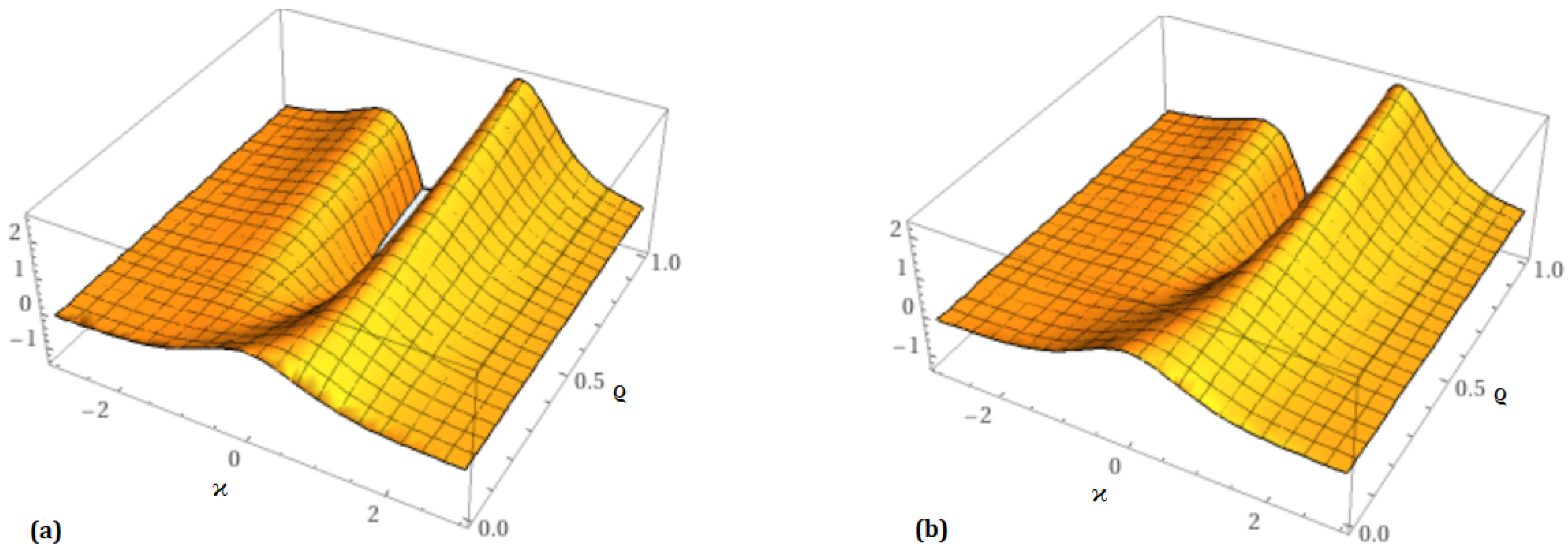
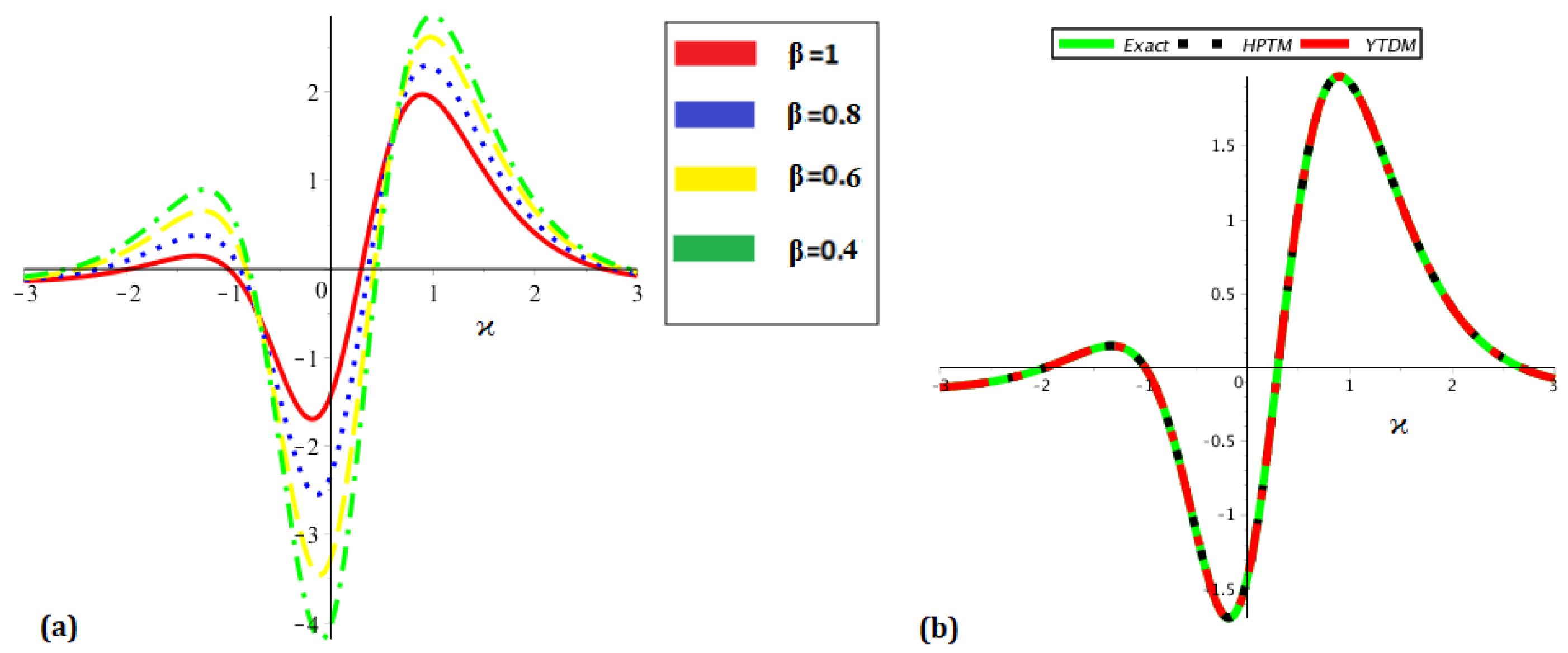
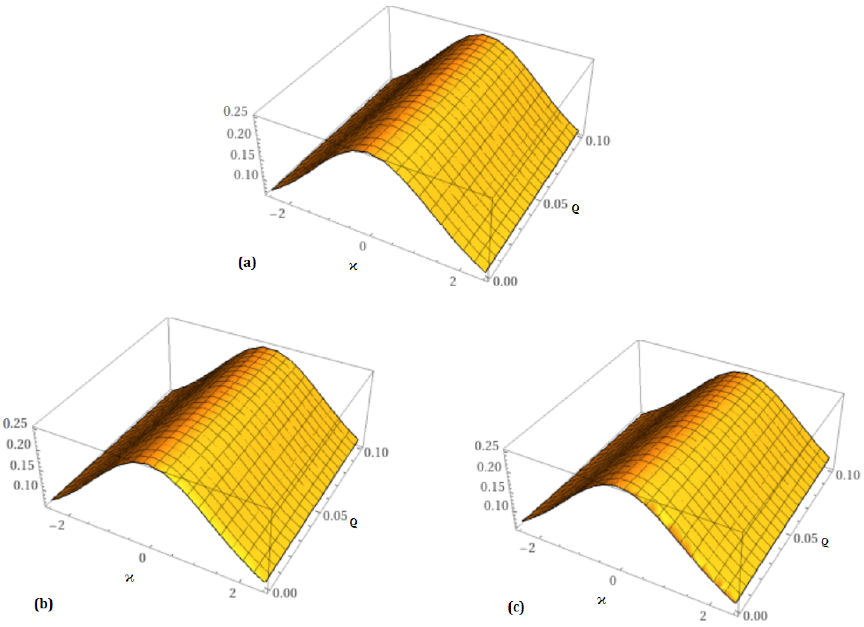
8. Physical Interpretation of Results

The findings and analysis for the analytical solution of the fractional CDG equations are shown in this part of the article. It is thought that the projected results rapidly approach the exact solution after a limited number of iterations. There are two components to the surface solution shown in Figure 1: (a) the accurate part and (b) the analytical part at $\beta =1$. Figure 2 provides (a) the analytical part of the surface solution at $\beta =0.60$ and (b) the analytical part of the surface solution at $\beta =0.80$. In the same way, Figure 3 is split into two sections: (a) the 2D analytical surface solution at various orders of $\beta$, and (b) the comparison surface solution of precise and analytical results.

Table 1. Analysis of the precise and analytical results at several $\beta$ orders.

$\mathit{\varkappa }$	$\mathit{\beta }=0.97$	$\mathit{\beta }=0.98$	$\mathit{\beta }=0.99$	$\mathit{\beta }=1$ (Appro)	$\mathit{\beta }=1$ (Exact)
0.0	0.8412492045	0.8412821476	0.8413116951	0.8413381923	0.8413382266
0.1	0.8347832441	0.8346459868	0.8345135197	0.8343858026	0.8343849486
0.2	0.8089819894	0.8086852743	0.8084011555	0.8081292105	0.8081276073
0.3	0.7658214625	0.7653876267	0.7649732281	0.7645774965	0.7645753904
0.4	0.7084342409	0.7078937677	0.7073781753	0.7068864044	0.7068840866
0.5	0.6406493580	0.6400366044	0.6394525467	0.6388959115	0.6388936545
0.6	0.5664939123	0.5658429627	0.5652228708	0.5646322278	0.5646302394
0.7	0.4897564694	0.4890978532	0.4884707464	0.4878736802	0.4878720841
0.8	0.4136762461	0.4130348823	0.4124244238	0.4118434074	0.4118422460
0.9	0.3407780718	0.3401724392	0.3395961584	0.3390478223	0.3390470757
1.0	0.2728373544	0.2722796467	0.2717490940	0.2712443819	0.2712439912

displays both the precise solution and the comparison of the analytical solution. We compare the absolute error of the third-order approximation with LRPSM, HASTM, and NTDM in

Table 2. Comparative analysis of the analytical solution with LRPSM, HASTM, and NTDM.

$\mathit{\varkappa }$	$\mathit{\varrho }$	Exact Solution	Our Methods Solution	Our Methods Error	LRPSM Error	HASTM Error	NTDM Error
0.5	0	0.6280127585	0.6280127585	0.0000000000	0.0000000000	0.0000000000	0.0000000000
	0.01	0.6388936545	0.6388959115	2.256967 $\times {10}^{-06}$	2.26691 $\times {10}^{-06}$	3.51211 $\times {10}^{-05}$	6.63723 $\times {10}^{-06}$
	0.02	0.6496327491	0.6496508562	1.810706 $\times {10}^{-05}$	1.81241 $\times {10}^{-05}$	2.81021 $\times {10}^{-04}$	7.7452 $\times {10}^{-05}$
	0.03	0.6602163246	0.6602775927	6.126800 $\times {10}^{-05}$	6.12895 $\times {10}^{-05}$	9.48603 $\times {10}^{-04}$	1.38205 $\times {10}^{-04}$
	0.04	0.6706305549	0.6707761209	1.455658 $\times {10}^{-04}$	1.45589 $\times {10}^{-04}$	2.24888 $\times {10}^{-03}$	1.17 $\times {10}^{-03}$
	0.05	0.6808615377	0.6811464403	2.849025$\times {10}^{-04}$	2.84925 $\times {10}^{-04}$	4.39294 $\times {10}^{-03}$	1.8875 $\times {10}^{-03}$
1.0	0	0.2615393671	0.2615393671	0.0000000000	0.0000000000	0.0000000000	0.0000000000
	0.01	0.2712439912	0.2712443819	3.906838$\times {10}^{-07}$	3.99819 $\times {10}^{-07}$	1.41429 $\times {10}^{-04}$	7.0112 $\times {10}^{-06}$
	0.02	0.2810871794	0.2810904023	3.222867 $\times {10}^{-06}$	3.23987 $\times {10}^{-06}$	2.24888 $\times {10}^{-03}$	2.78788 $\times {10}^{-05}$
	0.03	0.2910662174	0.2910774282	1.121086 $\times {10}^{-05}$	1.12342 $\times {10}^{-05}$	3.81193 $\times {10}^{-04}$	1.2331 $\times {10}^{-04}$
	0.04	0.3011780846	0.3012054598	2.737526 $\times {10}^{-05}$	2.74038 $\times {10}^{-05}$	9.02767 $\times {10}^{-04}$	1.1006 $\times {10}^{-03}$
	0.05	0.3114194433	0.3114744970	5.505375 $\times {10}^{-05}$	5.50858 $\times {10}^{-05}$	1.76163 $\times {10}^{-03}$	1.0116 $\times {10}^{-03}$

. The comparison shows a high degree of agreement between the analytical and exact results. Thus, compared to LRPSM, HASTM, and NTDM, the suggested strategies are dependable, innovative methods that need less calculation time and are simpler and more adaptable. Similarly, two diagrams are shown in Figure 4: (a) the precise surface solution and (b) the analytical surface solution at $\beta =1$. Figure 5 provides (a) the analytical part of the surface solution at $\beta =0.60$ and (b) the analytical part of the surface solution at $\beta =0.80$. Figure 6 shows (a) the 2D analytical surface solution at various orders of $\beta$ and (b) the comparison surface solution of precise and analytical results. The comparison among the exact and approximate solutions at different orders of $\beta$ is shown in

Table 3. Analysis of the precise and analytical results at several $\beta$ orders.

$\mathit{\varkappa }$	$\mathit{\beta }=0.97$	$\mathit{\beta }=0.98$	$\mathit{\beta }=0.99$	$\mathit{\beta }=1$ (Appro)	$\mathit{\beta }=1$ (Exact)
0.0	0.8412492045	0.8412821476	0.8413116951	0.8413381923	0.8413382266
0.1	0.8347832441	0.8346459868	0.8345135197	0.8343858026	0.8343849486
0.2	0.8089819894	0.8086852743	0.8084011555	0.8081292105	0.8081276073
0.3	0.7658214625	0.7653876267	0.7649732281	0.7645774965	0.7645753904
0.4	0.7084342409	0.7078937677	0.7073781753	0.7068864044	0.7068840866
0.5	0.6406493580	0.6400366044	0.6394525467	0.6388959115	0.6388936545
0.6	0.5664939123	0.5658429627	0.5652228708	0.5646322278	0.5646302394
0.7	0.4897564694	0.4890978532	0.4884707464	0.4878736802	0.4878720841
0.8	0.4136762461	0.4130348823	0.4124244238	0.4118434074	0.4118422460
0.9	0.3407780718	0.3401724392	0.3395961584	0.3390478223	0.3390470757
1.0	0.2728373544	0.2722796467	0.2717490940	0.2712443819	0.2712439912

. There are three components to the surface solution shown in Figure 7: (a) the analytical part at $\beta =1$, (b) $\beta =0.80$, and $\beta =0.60$. Figure 8 shows (a) the 2D analytical surface solution at various orders of $\beta$ and (b) the comparison surface solution of the analytical results. Additionally, the comparison among the exact and approximate solutions at different orders of $\beta$ is shown in

Table 4. Analysis of the precise and analytical results at several $\beta$ orders.

$\mathit{\varkappa }$	$\mathit{\beta }=0.96$	$\mathit{\beta }=0.97$	$\mathit{\beta }=0.98$	$\mathit{\beta }=0.99$	$\mathit{\beta }=1$
0.0	0.9602125488	0.9643569874	0.9680748874	0.9714095642	0.9744000000
0.1	0.9904392302	0.9925362180	0.9943131706	0.9958075547	0.9970528593
0.2	1.0014573480	1.0013532710	1.0010595720	1.0006050540	1.0000151990
0.3	0.9922549156	0.9899921951	0.9876807940	0.9853390759	0.9829829438
0.4	0.9634794619	0.9592829050	0.9551749023	0.9511628260	0.9472525522
0.5	0.9173351619	0.9115676279	0.9060098467	0.9006588122	0.8955109712
0.6	0.8572164277	0.8503175576	0.8437251030	0.8374271840	0.8314122178
0.7	0.7871841277	0.7796080070	0.7724064574	0.7655607516	0.7590531407
0.8	0.7114189494	0.7035832173	0.6961618533	0.6891314651	0.6824701346
0.9	0.6337652853	0.6260180752	0.6186998385	0.6117845694	0.6052480500
1.0	0.5574285929	0.5500337403	0.5430621488	0.5364869364	0.5302831645

. We note that the existing methods showed good agreement, providing an accurate solution to problems only after a few iterations. The rate of convergence demonstrates the validity of the provided methods for solving the suggested equations. This implies that any surface can be efficiently modeled in accordance with the necessary physical processes found in nature. Due to the well-known nonlocal nature of the Caputo fractional derivative, we can thus see that the order of the fractional derivative significantly affects the displacement profile. In the study of mathematical modeling of physical issues, the nonlocal aspect of the Caputo fractional derivative is crucial. Due to the fact that fractional operators have a memory effect, their use in mathematical modeling of physical systems has the primary benefit of better capturing the dynamic behavior of the system.

9. Conclusions

In this study, we used YTDM and HPTM techniques to examine a $CDG$ problem with a fractional order approximate solution. Readers can understand the procedures clearly since the implementation of YT directly transforms fractional derivative sections into algebraic terms in the given problems. The ADM and HPM techniques break down nonlinear components before they generate series solutions for the provided problems. The findings of the current study demonstrate that the techniques used to solve the fractional model under consideration are extremely valuable. The outcomes attained illustrated the highest degree of agreement with respect to the precise solutions of the proposed problems. It was demonstrated through the use of the suggested approaches to test problems that the mathematical model of non-integer order could interpret any experimental results more precisely than the integer-order model. Both approaches demonstrate that results and exact solutions are very similar, and the acquired solutions are displayed graphically and numerically. The utilized approaches yield extremely exact results with little computational effort. We have noticed that the fractional results converge to the integer-order solution for the proposed problems as the fractional order approaches the integer order. Several numerical comparisons are made with well-known analytical methods and the exact solutions when $\beta =1$. It is evident from the comparison that the proposed methods outperformed other methods in handling the CDG equations considered in this paper. As a result, we emphasize that the recommended approaches are very accurate and efficient methods for solving the fractional $CDG$ model with better physical aspects. The analysis in this work focused exclusively on time-fractional non-linear PDEs existing in one-dimensional conditions. The forthcoming work will advance the methodology to apply it to space–time fractional PDEs throughout multiple dimensional spaces while also handling space fractional PDEs. The use of Caputo fractional order derivatives allows researchers to solve nonlinear real-world problems. Researchers can expand these investigations to incorporate additional fractional derivatives, including Caputo–Fabrizio, conformable, and Atangana–Baleanu derivatives. This work is helpful and opens up new possibilities for the sciences and engineering.

References

1. Khatun, M.A.; Arefin, M.A.; Uddin, M.H.; İnç, M.; Akbar, M.A. An analytical approach to the solution of fractional-coupled modified equal width and fractional-coupled Burgers equations. J. Ocean. Eng. Sci. 2022, in press.
2. Zaman, U.H.M.; Arefin, M.A.; Akbar, M.A.; Uddin, M.H. Analyzing numerous travelling wave behavior to the fractional-order nonlinear Phi-4 and Allen-Cahn equations throughout a novel technique. Results Phys. 2022, 37, 105486. [Google Scholar]
3. Podlubny, I. Fractional Differential Equations; Academic Press: New York, NY, USA, 1999; Volume 198. [Google Scholar]
4. Miller, K.S.; Ross, B. An Introduction to the Fractional Calculus and Fractional Differential Equations; John Wiley and Sons: New York, NY, USA, 1993. [Google Scholar]
5. Oldham, K.B.; Spanier, J. The Fractional Calculus: Theory and Applications of Differentiation and Integration to Arbitrary Order; Academic Press: New York, NY, USA, 1974. [Google Scholar]
6. Kilbas, A.A.; Srivastava, H.M.; Trujillo, J.J. Theory and Applications of Fractional Differential Equations; Elsevier: Amsterdam, The Netherlands, 2006. [Google Scholar]
7. Saad, K.M. Comparative study on Fractional Isothermal Chemical Model. Alex. Eng. J. 2021, 60, 3265–3274. [Google Scholar]
8. Saad, K.M.; Alqhtani, M. Numerical simulation of the fractal-fractional reaction diffusion equations with general nonlinear. AIMS Math. 2021, 6, 3788–3804. [Google Scholar]
9. Loyinmi, A.C.; Gbodogbe, S.O.; Idowu, K.O. On the interaction of the human immune system with foreign body: Mathematical modeling approach. Kathmandu Univ. J. Sci. Eng. Technol. 2023, 17. [Google Scholar] [CrossRef]
10. Ganie, A.H.; Mofarreh, F.; Khan, A. On new computations of the time-fractional nonlinear KdV-Burgers equation with exponential memory. Phys. Scr. 2024, 99, 045217. [Google Scholar]
11. Ganie, A.H.; Mallik, S.; AlBaidani, M.M.; Khan, A.; Shah, M.A. Novel analysis of nonlinear seventh-order fractional Kaup-Kupershmidt equation via the Caputo operator. Bound. Value Probl. 2024, 2024, 87. [Google Scholar]
12. Ganie, A.H.; Mofarreh, F.; Khan, A. A fractional analysis of Zakharov-Kuznetsov equations with the Liouville-Caputo operator. Axioms 2023, 12, 609. [Google Scholar] [CrossRef]
13. Mishra, N.K.; AlBaidani, M.M.; Khan, A.; Ganie, A.H. Two novel computational techniques for solving nonlinear time-fractional Lax’s Korteweg-de Vries equation. Axioms 2023, 12, 400. [Google Scholar] [CrossRef]
14. El-Ajou, A.; Saadeh, R.; Dunia, M.A.; Qazza, A.; Al-Zhour, Z. A new approach in handling one-dimensional time-fractional Schrödinger equations. AIMS Math. 2024, 9, 10536–10560. [Google Scholar]
15. AlBaidani, M.M.; Ganie, A.H.; Khan, A. The dynamics of fractional KdV type equations occurring in magneto-acoustic waves through non-singular kernel derivatives. AIP Adv. 2023, 13, 115215. [Google Scholar] [CrossRef]
16. AlBaidani, M.M.; Aljuaydi, F.; Alharthi, N.S.; Khan, A.; Ganie, A.H. Study of fractional forced KdV equation with Caputo-Fabrizio and Atangana-Baleanu-Caputo differential operators. AIP Adv. 2024, 14, 015340. [Google Scholar] [CrossRef]
17. Ganie, A.H.; AlBaidani, M.M.; Khan, A. A comparative study of the fractional partial differential equations via novel transform. Symmetry 2023, 15, 1101. [Google Scholar] [CrossRef]
18. Hirota, R. The Direct Method in Soliton Theory; Cambridge University Press: Cambridge, UK, 2004. [Google Scholar]
19. Hirota, R. Exact Solutions of the Sine-Gordon Equation for Multiple Collisions of Solitons. J. Phys. Soc. Jpn. 1972, 33, 1459–1463. [Google Scholar] [CrossRef]
20. Hietarinta, J. A Search for Bilinear Equations Passing Hirota’s Three-Soliton Condition. I. KdV-Type Bilinear Equations. J. Math. Phys. 1987, 28, 1732–1742. [Google Scholar] [CrossRef]
21. Fan, E.; Zhang, J. Applications of the Jacobi elliptic function method to special-type nonlinear equations. Phys. Lett. A 2002, 305, 383–392. [Google Scholar] [CrossRef]
22. Malfliet, W.; Hereman, W. The tanh method: I. Exact solutions of nonlinear evolution and wave equations. Phys. Scr. 1996, 54, 563. [Google Scholar] [CrossRef]
23. Salupere, A. The pseudospectral method and discrete spectral analysis. In Applied Wave Mathematics: Selected Topics in Solids, Fluids, and Mathematical Methods; Springer: Berlin/Heidelberg, Germany, 2009; pp. 301–333. [Google Scholar]
24. Zhang, S.L.; Wu, B.; Lou, S.Y. Painlevé analysis and special solutions of generalized Broer-Kaup equations. Phys. Lett. A 2002, 300, 40–48. [Google Scholar] [CrossRef]
25. Oqielat, M.A.N.; Eriqat, T.; Al-Zhour, Z.; El-Ajou, A.; Odibat, Z. Laplace Residual Power Series Solutions of the Fractional Modified KdV System with Physical Applications. Int. J. Appl. Comput. Math. 2025, 11, 12. [Google Scholar] [CrossRef]
26. Yadav, J.U.; Singh, T.R. Alternative Variational Iteration Elzaki Transform Method for Solving Time-Fractional Generalized Burgers-Fisher Equation in Porous Media Flow Modeling. Math. Methods Appl. Sci. 2025, 2025. [Google Scholar] [CrossRef]
27. Aboodh, K.S. Solving porous medium equation using Aboodh transform homotopy perturbation method. Am. J. Appl. Math. 2016, 4, 271–276. [Google Scholar] [CrossRef]
28. Gao, H.; Pandey, R.K.; Lodhi, R.K.; Jafari, H. Solution of Time-Fractional Black-Scholes Equations via Homotopy Analysis Sumudu Transform Method. Fractals 2025. [Google Scholar] [CrossRef]
29. Wang, P.; Feng, X.; He, S. A q-homotopy analysis transformation method for solving (2+1)-dimensional coupled fractional nonlinear Schrodinger equations. Int. J. Geom. Methods Mod. Phys. 2025. [Google Scholar] [CrossRef]
30. Ganie, A.H.; Khan, A.; Alharthi, N.S.; Tolasa, F.T.; Jeelani, M.B. Comparative Analysis of Time-Fractional Coupled System of Shallow-Water Equations Including Caputo’s Fractional Derivative. J. Math. 2024, 2024, 2440359. [Google Scholar] [CrossRef]
31. Ganie, A.H.; Mofarreh, F.; Alharthi, N.S.; Khan, A. Novel computations of the time-fractional chemical Schnakenberg mathematical model via non-singular kernel operators. Bound. Value Probl. 2025, 2025, 2. [Google Scholar]
32. Aychluh, M.; Ayalew, M. The Fractional Power Series Method for Solving the Nonlinear Kuramoto-Sivashinsky Equation. Int. J. Appl. Comput. Math. 2025, 11, 29. [Google Scholar] [CrossRef]
33. Awadalla, M.; Ganie, A.H.; Fathima, D.; Khan, A.; Alahmadi, J. A mathematical fractional model of waves on Shallow water surfaces: The Korteweg-de Vries equation. AIMS Math. 2024, 9, 10561–10579. [Google Scholar]
34. Dodd, R.K.; Gibbon, J.D. The prolongation structure of a higher order Korteweg-de Vries equation. Proc. R. Soc. Lond. A 1977, 358, 287–296. [Google Scholar]
35. Caputo, M. Linear models of Dissipation whose Q is almost Frequency independent II. Geophys. J. R. Astr. Soc. 1967, 13, 529–539. [Google Scholar]
36. Caudrey, P.J.; Dodd, R.K.; Gibbon, J.D. A new hierarchy of Korteweg-de Vries equations. Proc. R. Soc. Lond. A 1976, 351, 407–422. [Google Scholar]
37. Singh, H.; Kumar, D.; Pandey, R.K. An efficient computational method for the time-space fractional Klein-Gordon equation. Front. Phys. 2020, 8, 281. [Google Scholar]
38. He, J.-H. Homotopy Perturbation Technique. Comput. Methods Appl. Mech. Eng. 1999, 178, 257–262. [Google Scholar]
39. He, J.-H. Variational Iteration Method—A kind of nonlinear analytical technique: Some examples. Int. J. Non-Linear Mech. 1999, 34, 699–708. [Google Scholar]
40. Adomian, G. (Ed.) Solving Frontier Problems of Physics: The Decomposition Method; Springer: Dordrecht, The Netherlands, 1994. [Google Scholar]
41. Jin, L. Application of the Variational Iteration Method for solving the fifth order Caudrey-Dodd-Gibbon Equation. Int. Math. Forum 2010, 5, 3259–3265. [Google Scholar]
42. Wazwaz, A.M. Analytical study of the fifth order integrable nonlinear evolution equations by using the tanh method. Appl. Math. Comput. 2006, 174, 289–299. [Google Scholar]
43. Xu, Y.-G.; Zhou, X.-W.; Yao, L. Solving the fifth order Caudrey- Dodd-Gibbon (CDG) equation using the exp-function method. Appl. Math. Comput. 2008, 206, 70–73. [Google Scholar]
44. Wazwaz, A.M. Multiple-soliton solutions for the fifth order Caudrey-Dodd-Gibbon (CDG) equation. Appl. Math. Comput. 2008, 197, 719–724. [Google Scholar]
45. Podlubny, I.; Kacenak, M. Isoclinal matrices and numerical solution of fractional differential equations. In Proceedings of the 2001 European Control Conference (ECC), Porto, Portugal, 4–7 September 2001. [Google Scholar]
46. Yang, X.J.; Baleanu, D.; Srivastava, H.M. Local fractional laplace transform and applications. In Local Fractional Integral Transforms and Their Applications; Elsevier: Amsterdam, The Netherlands, 2016; p. 147178. [Google Scholar]
47. Cooper, G.J. Error bounds for numerical solutions of ordinary differential equations. Numer. Math. 1971, 18, 162–170. [Google Scholar]
48. Warne, P.G.; Warne, D.P.; Sochacki, J.S.; Parker, G.E.; Carothers, D.C. Explicit a-priori error bounds and adaptive error control for approximation of nonlinear initial value differential systems. Comput. Math. Appl. 2006, 52, 1695–1710. [Google Scholar]
49. Yüzbaşi, Ş. A numerical approach for solving a class of the nonlinear Lane-Emden type equations arising in astrophysics. Math. Methods Appl. Sci. 2011, 34, 2218–2230. [Google Scholar]
Figure 1. Exact solution as well as analytical solution behavior at β = 1 .
Fractalfract 09 00199 g001
Figure 2. Analytical solution behavior of w ( ϰ , ϱ ) at (a) β = 0.6 and (b) β = 0.8 .
Fractalfract 09 00199 g002
Figure 3. Analytical solution behavior of w ( ϰ , ϱ ) at (a) different values of β , and (b) a comparison among accurate and analytical solutions.
Fractalfract 09 00199 g003
Figure 4. Exact solution as well as analytical solution behavior at β = 1 .
Fractalfract 09 00199 g004
Figure 5. Analytical solution behavior of w ( ϰ , ϱ ) at (a) β = 0.6 and (b) β = 0.8 .
Fractalfract 09 00199 g005
Figure 6. Analytical solution behavior of w ( ϰ , ϱ ) at (a) different values of β , and (b) a comparison among accurate and analytical solutions.
Fractalfract 09 00199 g006
Figure 7. Analytical solution behavior of w ( ϰ , ϱ ) at (a) β = 1 , (b) β = 0.80 and (c) β = 0.60 .
Fractalfract 09 00199 g007
Figure 8. Analytical solution behavior of w ( ϰ , ϱ ) at (a) different values of β , and (b) a comparison among accurate and analytical solutions.
Fractalfract 09 00199 g008