Investigation of New Optical Solutions for the Fractional Schrödinger Equation with Time-Dependent Coefficients: Polynomial, Random, Trigonometric, and Hyperbolic Functions

Abstract

The fractional Schrödinger equation with time-dependent coefficients (FSE-TDCs) is taken into consideration here. The mapping method and the $(G^{\prime }/G)$-expansion method are applied to generate new bright solutions, kink solutions, dark optical solutions, singular solutions, periodic solutions, and others. Because the Schrödinger equation is widely employed in quantum computers, quantum mechanics, physics, engineering, and chemistry, the solutions developed can be utilized to examine a wide range of important physical phenomena. In addition, we illustrate the influence of the coefficients, when these coefficients have specific values, such as random, polynomial, trigonometric, and hyperbolic functions, on the exact solutions of FSE-TDCs. Also, we show the influence of fractional-order derivatives on the obtained solutions.

1. Introduction

Fractional differential equations with variable coefficients (FDEs-VCs) are a subfield of mathematics that deals with equations with fractional derivatives in which the coefficients are not constant but vary based on the independent variables. These equations are utilized in a variety of areas, for example, engineering, physics, and finance [1,2,3,4,5], where the dynamics of the systems under consideration are not easily described by traditional differential equations.

One of the main features of FDEs-VCs is that they give a more accurate account of the behavior of specific systems than integer-order differential equations with constant coefficients. This is because fractional derivatives account for the memory effects and long-range interactions seen in many physical systems, allowing for a more realistic description of their dynamics. The variable coefficients further enhance the flexibility of the model, capturing the changing nature of the system over time.

In terms of solving FDEs-VCs, the approaches might be more difficult than regular differential equations. This is due to the nonlinearity and non-integer order of the derivatives involved, as well as the variability of the coefficients. In recent years, many effective and useful methods for solving these equations have been proposed, such as Hirota’s bilinear approach [6], solitary wave ansatz [7], the mapping method [8], $(G^{\prime }/G^2)$-expansion and Jacobian elliptic functions methods [9], the $(G^{\prime }/G)$-expansion method [10], the sub-equation method [11], the bilinear neural network method [12,13], the bilinear residual network method [14,15], and the nonlinear compact-polynomial computational scheme [16].

In this study, we consider the fractional Schrödinger equation (FSE) with time-dependent coefficients (TDCs):

$$i{\mathcal{U}}_t+\theta \left(t\right){\mathcal{T}}_{xx}^{\alpha ,\delta }\mathcal{U}+\kappa \left(t\right){\left|\mathcal{U}\right|}^2\mathcal{U}=0,$$

(1)

where $\mathcal{U}=\mathcal{U}(x,t)$ indicates the wave profile, $i=\sqrt{-1}$, ${\left|\mathcal{U}\right|}^2\mathcal{U}$ is the Kerr law of nonlinearity, ${\mathcal{U}}_{xx}$ is the group velocity dispersion, ${\mathcal{T}}^{\alpha ,\delta }$ is the M-truncated derivative operator, and $\theta \left(t\right)$ and $\kappa \left(t\right)$ are arbitrary functions depending on t.

The Schrödinger Equation (1) with $\alpha =1,$ and $\delta =0$ is a powerful tool that has enabled incredible advancements in physics, chemistry, and computer science. Its applications range from predicting the behavior of electrons in atoms to revolutionizing the field of quantum computing. As we continue to explore the implications of quantum mechanics and develop new technologies based on its principles, the Schrödinger equation will remain a fundamental equation that shapes our understanding of the universe.

Because of the importance of the Schrödinger Equation (1), many authors, for example [17,18,19,20], have investigated the uniqueness and existence of solutions or approximate solutions for various type of the stochastic Schrödinger equation. Moreover, there are other authors, such as [21,22,23,24,25], who have obtained the solutions of Equation (1).

The originality of this paper concerns finding the analytical solutions of the FSE-TDCs (1). Elliptic, trigonometric, hyperbolic, and rational functions are just a few of the many solutions we may obtain by using the mapping method and the ($G^{\prime }/G)$-expansion method. We generalize many previous results, such as those reported in [24,25]. Furthermore, we utilize Matlab tools to present 3D and 2D figures for some of the established solutions of the FSE-TDCs (1) to examine the impact of the M-truncated derivative and the time-dependent coefficient, when these coefficients have specific values, such as random, polynomial, trigonometric, and hyperbolic functions.

This is how the article is structured. In Section 2, we state the definition of MTD and its features. In Section 3, we apply an appropriate transformation to obtain the wave equation of the FSE-TDCs (1). In Section 4, we use two methods to construct the analytical solutions of the FSE-TDCs (1). In Section 5, we address how the derived solutions are impacted by the TDCs and MTD. Lastly, the article’s conclusion is stated.

2. M-Truncated Derivative

Fractional derivative operators are important in many fields of science and engineering because they can better simulate the behavior of complicated systems than integer-order derivatives. There exist various kinds of fractional derivative operators, for instance, the Hadamard derivative, the Grünwald–Letnikov derivative, the Caputo derivative, the Jumarie derivative, the Riemann–Liouville derivative, and the Katugampola derivative [26,27,28,29]. Recently, Sousa et al. [30] presented a new derivative that naturally develops from the traditional derivative, called the M-truncated derivative (MTD). The quotient rule, product rule, linearity, composition rule, and chain rule are among the traditional calculus characteristics that are present in the MTD. The MTD of order $0<\alpha \le 1$ for $\mathcal{U}:[0,\infty )\to \mathbb{R}$ is defined by

$${\mathcal{T}}_x^{\alpha ,\delta }\mathcal{U}\left(x\right)=\underset{h\to 0}{lim}{\displaystyle \frac{\mathcal{U}\left(x{\mathcal{E}}_{k,\delta }\left(h{x}^{-\alpha }\right)\right)-\mathcal{U}\left(x\right)}{h}},$$

where

$${\mathcal{E}}_{k,\delta }\left(\varphi \right)=\sum _{j=0}^k{\displaystyle \frac{{\varphi }^j}{\Gamma (\delta j+1)}},\mathrm{for}\delta >0\mathrm{and}\varphi \in \mathbb{C}.$$

The MTD satisfies the following features [30] for $c_1$ and $c_2$ are real constants:

(1) ${\mathcal{T}}_x^{\alpha ,\delta }(c_1\mathcal{U}+c_2\mathcal{V})=c_1{\mathcal{T}}_x^{\alpha ,\delta }\mathcal{U}+c_2{\mathcal{T}}_x^{\alpha ,\delta }\mathcal{V},$

(2) ${\mathcal{T}}_x^{\alpha ,\delta }\left(x^{\nu }\right)={\displaystyle \frac{\nu }{\Gamma (\delta +1)}}{x}^{\nu -\alpha },$

(3) ${\mathcal{T}}_x^{\alpha ,\delta }\left(\mathcal{VU}\right)={\mathcal{VT}}_x^{\alpha ,\delta }\mathcal{U}+{\mathcal{UT}}_x^{\alpha ,\delta }\mathcal{V},$

(4)${\mathcal{T}}_x^{\alpha ,\delta }\mathcal{U}\left(x\right)={\displaystyle \frac{x^{1-\alpha }}{\Gamma (\delta +1)}}{\displaystyle \frac{d\mathcal{U}}{dx}},$

(5) ${\mathcal{T}}_x^{\alpha ,\delta }(\mathcal{U}\circ \mathcal{V})\left(x\right)={\mathcal{U}}^{\prime }\left(\mathcal{V}\left(x\right)\right){\mathcal{T}}_x^{\alpha ,\delta }\mathcal{U}\left(x\right),$

3. Wave Equation for FSE-TDCs

The following transformation is applied to find the wave equation for the FSE-TDCs (1):

$$\mathcal{U}(x,t)=\mathcal{G}\left({\mu }_{\alpha }\right){\mathrm{e}}^{i{\psi }_{\alpha }},$$

(2)

$${\mu }_{\alpha }={\displaystyle \frac{\mu \Gamma (1+\delta )}{\alpha }}{x}^{\alpha }+{\int }_0^{t}f\left(\tau \right)d\tau ,\mathrm{and}{\psi }_{\alpha }={\displaystyle \frac{\rho \Gamma (1+\delta )}{\alpha }}{x}^{\alpha }+{\int }_0^{t}g\left(\tau \right)d\tau ,$$

where $\mathcal{G}$ indicates a real function. Putting Equation (2) into Equation (1) and utilizing

$$\begin{array}{ccc}\hfill {\mathcal{U}}_t& =& [f\left(t\right){\mathcal{G}}^{\prime }+ig\left(t\right)\mathcal{G}]{\mathrm{e}}^{i{\psi }_{\alpha }},\hfill \\ \hfill {\mathcal{T}}_{xx}^{\alpha ,\delta }\mathcal{W}& =& [{\mu }^2{\mathcal{G}}^{″}+2i\rho \mu {\mathcal{G}}^{\prime }-{\rho }^2\mathcal{G}]{\mathrm{e}}^{i{\psi }_{\alpha }},\hfill \end{array}$$

we have for the real part

$${\mathcal{G}}^{″}-{\hslash }_1\left(t\right)\mathcal{G}+{\hslash }_2\left(t\right){\mathcal{G}}^3=0,$$

(3)

and for the imaginary part

$$[2\rho \mu \theta \left(t\right)+f\left(t\right)]{\mathcal{G}}^{\prime }=0,$$

(4)

where

$${\hslash }_1\left(t\right)={\displaystyle \frac{g\left(t\right)+{\rho }^2\theta \left(t\right)}{{\mu }^2\theta \left(t\right)}}\mathrm{and}{\hslash }_2\left(t\right)={\displaystyle \frac{\kappa \left(t\right)}{{\mu }^2\theta \left(t\right)}}.$$

(5)

From (4), we obtain

$$f\left(t\right)=-2\rho \mu \theta \left(t\right).$$

(6)

4. Exact Solutions of FSE-TDCs Equation

To obtain the solutions of Equation (3), we employ two different methods. These methods are the mapping method [31] and the ($G^{\prime }/G)$-expansion method [32]. Next, we obtain the solutions to the FSH Equation (1) by applying the transformation (2).

4.1. Mapping Method

Here, we utilize the mapping method reported in [31]. Let the solutions of Equation (3) have the form

$$\mathcal{G}\left({\mu }_{\alpha }\right)=\sum _{i=1}^n{\mathsf{\ell }}_i{\mathcal{P}}^i\left({\mu }_{\alpha }\right),{\mathsf{\ell }}_M\ne 0,$$

(7)

By equating ${\mathcal{G}}^3$ with ${\mathcal{G}}^{″}$ in Equation (3), we have the value of n as

$$3n=n+2\Rightarrow n=1.$$

(8)

Rewriting Equation (7), with $n=1$, as

$$\mathcal{G}\left({\mu }_{\alpha }\right)={\mathsf{\ell }}_0+{\mathsf{\ell }}_1\mathcal{P}\left({\mu }_{\alpha }\right),$$

(9)

where ${\mathsf{\ell }}_1\ne 0$ and $\mathcal{P}$ solves

$${\mathcal{P}}^{\prime }=\sqrt{{\gamma }_1{\mathcal{P}}^4+{\gamma }_2{\mathcal{P}}^2+{\gamma }_3},$$

(10)

where ${\gamma }_1,{\gamma }_2$, and ${\gamma }_3$ are real constants. Differentiating Equation (9) twice and using (10), we have

$${\mathcal{G}}^{″}={\mathsf{\ell }}_1({\gamma }_2\mathcal{P}+2{\gamma }_1{\mathcal{P}}^3).$$

(11)

Inserting Equations (9) and (11) into Equation (3), we have

$$(2{\mathsf{\ell }}_1{\gamma }_1+{\hslash }_2{\mathsf{\ell }}_1^3){\mathcal{P}}^3+3{\hslash }_2{\mathsf{\ell }}_0{\mathsf{\ell }}_1^2{\mathcal{P}}^2+({\mathsf{\ell }}_1{\gamma }_2+3{\hslash }_2{\mathsf{\ell }}_0^2{\mathsf{\ell }}_1-{\mathsf{\ell }}_1{\hslash }_1)\mathcal{P}+({\hslash }_2{\mathsf{\ell }}_0^3-{\hslash }_1{\mathsf{\ell }}_0)=0.$$

Setting each coefficient of ${\mathcal{P}}^k$ equal zero, we obtain the system:

$$2{\mathsf{\ell }}_1{\gamma }_1+{\hslash }_2{\mathsf{\ell }}_1^3=0,$$

$$3{\hslash }_2{\mathsf{\ell }}_0{\mathsf{\ell }}_1^2=0,$$

$${\mathsf{\ell }}_1{\gamma }_2+3{\hslash }_2{\mathsf{\ell }}_0^2{\mathsf{\ell }}_1-{\mathsf{\ell }}_1{\hslash }_1=0,$$

and

$${\hslash }_2{\mathsf{\ell }}_0^3-{\hslash }_1{\mathsf{\ell }}_0=0.$$

When the previous system is solved for ${\mathsf{\ell }}_1\ne 0$, we obtain

$${\mathsf{\ell }}_0=0,{\mathsf{\ell }}_1=\pm \sqrt{{\displaystyle \frac{-2{\gamma }_1}{{\hslash }_2}}},{\gamma }_2={\hslash }_1.$$

(12)

By using (5) and (6), we have

$${\mathsf{\ell }}_0=0,{\mathsf{\ell }}_1=\pm \sqrt{{\displaystyle \frac{-2{\mu }^2{\gamma }_1\theta \left(t\right)}{\kappa \left(t\right)}}},f\left(t\right)=-2\rho \mu \theta \left(t\right),\mathrm{and}g\left(t\right)=({\mu }^2{\gamma }_2-{\rho }^2)\theta \left(t\right).$$

Hence, by using Equations (2), (9) and (12), the FSE-TDCs (1) possess the solution

$$\mathcal{U}(x,t)=\pm \sqrt{{\displaystyle \frac{-2{\mu }^2{\gamma }_1\theta \left(t\right)}{\kappa \left(t\right)}}}\mathcal{P}\left({\mu }_{\alpha }\right){\mathrm{e}}^{i{\psi }_{\alpha }}\mathrm{for}{\displaystyle \frac{\theta \left(t\right)}{\kappa \left(t\right)}}<0,$$

(13)

where ${\mu }_{\alpha }={\displaystyle \frac{\mu \Gamma (1+\delta )}{\alpha }}{x}^{\alpha }-2\rho \mu {\int }_0^t\theta \left(\tau \right)d\tau$ and ${\psi }_{\alpha }={\displaystyle \frac{\rho \Gamma (1+\delta )}{\alpha }}{x}^{\alpha }+({\mu }^2{\gamma }_2-{\rho }^2){\int }_0^t\theta \left(\tau \right)d\tau$.

There are many cases based on ${\gamma }_1$:

Case 1: If ${\gamma }_1={Ķ}^2,{\gamma }_2=-(1+{Ķ}^2)$, and ${\gamma }_3=1,$ then $\mathcal{P}\left({\mu }_{\alpha }\right)=sn\left({\mu }_{\alpha }\right).$ Thus, the FSE-TDCs (1), utilizing Equation (13), possess the solution

$$\mathcal{U}(x,t)=\pm Ķ\sqrt{{\displaystyle \frac{-2{\mu }^2\theta \left(t\right)}{\kappa \left(t\right)}}}sn\left({\mu }_{\alpha }\right){\mathrm{e}}^{i{\psi }_{\alpha }}\mathrm{for}{\displaystyle \frac{\theta \left(t\right)}{\kappa \left(t\right)}}<0.$$

(14)

When Ķ$\to 1,$ Equation (14) changes to

$$\mathcal{U}(x,t)=\pm \sqrt{{\displaystyle \frac{-2{\mu }^2\theta \left(t\right)}{\kappa \left(t\right)}}}tanh\left({\mu }_{\alpha }\right){\mathrm{e}}^{i{\psi }_{\alpha }}\mathrm{for}{\displaystyle \frac{\theta \left(t\right)}{\kappa \left(t\right)}}<0.$$

(15)

Case 2: If ${\gamma }_1=1,{\gamma }_2=2{Ķ}^2-1$, and ${\gamma }_3=-{Ķ}^2(1-{Ķ}^2)$, then $\mathcal{P}\left({\mu }_{\alpha }\right)=ds\left({\mu }_{\alpha }\right)$. Thus, the FSE-TDCs (1), utilizing Equation (13), possess the solution

$$\mathcal{U}(x,t)=\pm \sqrt{{\displaystyle \frac{-2{\mu }^2\theta \left(t\right)}{\kappa \left(t\right)}}}ds\left({\mu }_{\alpha }\right){\mathrm{e}}^{i{\psi }_{\alpha }}\mathrm{for}{\displaystyle \frac{\theta \left(t\right)}{\kappa \left(t\right)}}<0.$$

(16)

If Ķ$\to 1,$ Equation (16) changes to

$$\mathcal{U}(x,t)=\pm \sqrt{{\displaystyle \frac{-2{\mu }^2\theta \left(t\right)}{\kappa \left(t\right)}}}\mathrm{csch}\left({\mu }_{\alpha }\right){\mathrm{e}}^{i{\psi }_{\alpha }}\mathrm{for}{\displaystyle \frac{\theta \left(t\right)}{\kappa \left(t\right)}}<0.$$

(17)

If Ķ$\to 0,$ Equation (16) tends to

$$\mathcal{U}(x,t)=\pm \sqrt{{\displaystyle \frac{-2{\mu }^2\theta \left(t\right)}{\kappa \left(t\right)}}}csc\left({\mu }_{\alpha }\right){\mathrm{e}}^{i{\psi }_{\alpha }}\mathrm{for}{\displaystyle \frac{\theta \left(t\right)}{\kappa \left(t\right)}}<0.$$

(18)

Case 3: When ${\gamma }_1=1,{\gamma }_2=2-{Ķ}^2$, and ${\gamma }_3=(1-{Ķ}^2),$ then $\mathcal{P}\left({\mu }_{\alpha }\right)=cs\left({\mu }_{\alpha }\right).$ Thus, the FSE-TDCs (1), utilizing Equation (13), possess the solution

$$\mathcal{U}(x,t)=\pm \sqrt{{\displaystyle \frac{-2{\mu }^2\theta \left(t\right)}{\kappa \left(t\right)}}}cs\left({\mu }_{\alpha }\right){\mathrm{e}}^{i{\psi }_{\alpha }}\mathrm{for}{\displaystyle \frac{\theta \left(t\right)}{\kappa \left(t\right)}}<0.$$

(19)

If Ķ$\to 1$, then Equation (19) tends to

$$\mathcal{U}(x,t)=\pm \sqrt{{\displaystyle \frac{-2{\mu }^2\theta \left(t\right)}{\kappa \left(t\right)}}}\mathrm{csch}\left({\mu }_{\alpha }\right){\mathrm{e}}^{i{\psi }_{\alpha }}\mathrm{for}{\displaystyle \frac{\theta \left(t\right)}{\kappa \left(t\right)}}<0.$$

(20)

When Ķ$\to 0$, Equation (19) changes to

$$\mathcal{U}(x,t)=\pm \sqrt{{\displaystyle \frac{-2{\mu }^2\theta \left(t\right)}{\kappa \left(t\right)}}}cot\left({\mu }_{\alpha }\right){\mathrm{e}}^{i{\psi }_{\alpha }}\mathrm{for}{\displaystyle \frac{\theta \left(t\right)}{\kappa \left(t\right)}}<0.$$

(21)

Case 4: If ${\gamma }_1={\displaystyle \frac{{Ķ}^2}{4}},{\gamma }_2={\displaystyle \frac{({Ķ}^2-2)}{2}}$, and ${\gamma }_3={\displaystyle \frac{1}{4}},$ then $\mathcal{P}\left({\mu }_{\alpha }\right)=nc\left({\mu }_{\alpha }\right)+sc\left({\mu }_{\alpha }\right).$ So, the FSE-TDCs (1), utilizing Equation (13), possess the solution

$$\mathcal{U}(x,t)=\pm {\displaystyle \frac{Ķ}{2}}\sqrt{{\displaystyle \frac{-2{\mu }^2\theta \left(t\right)}{\kappa \left(t\right)}}}(nc\left({\mu }_{\alpha }\right)+sc\left({\mu }_{\alpha }\right)){\mathrm{e}}^{i{\psi }_{\alpha }}\mathrm{for}{\displaystyle \frac{\theta \left(t\right)}{\kappa \left(t\right)}}<0.$$

(22)

If Ķ$\to 1,$ then Equation (22) changes to

$$\mathcal{U}(x,t)=\pm {\displaystyle \frac{1}{2}}\sqrt{{\displaystyle \frac{-2{\mu }^2\theta \left(t\right)}{\kappa \left(t\right)}}}(cosh\left({\mu }_{\alpha }\right)+sinh\left({\mu }_{\alpha }\right)){\mathrm{e}}^{i{\psi }_{\alpha }}\mathrm{for}{\displaystyle \frac{\theta \left(t\right)}{\kappa \left(t\right)}}<0.$$

(23)

Case 5: If ${\gamma }_1={\displaystyle \frac{{(1-{Ķ}^2)}^2}{4}},{\gamma }_2={\displaystyle \frac{{(1-{Ķ}^2)}^2}{2}}$, and ${\gamma }_3={\displaystyle \frac{1}{4}},$ then $\mathcal{P}\left({\mu }_{\alpha }\right)={\displaystyle \frac{sn\left({\mu }_{\alpha }\right)}{dn\left({\mu }_{\alpha }\right)+cn\left({\mu }_{\alpha }\right)}}$. Therefore, the FSE-TDCs (1), utilizing Equation (13), possess the solution

$$\mathcal{U}(x,t)=\pm {\displaystyle \frac{(1-{Ķ}^2)}{2}}\sqrt{{\displaystyle \frac{-2{\mu }^2\theta \left(t\right)}{\kappa \left(t\right)}}}[{\displaystyle \frac{sn\left({\mu }_{\alpha }\right)}{dn\left({\mu }_{\alpha }\right)+cn\left({\mu }_{\alpha }\right)}}]{\mathrm{e}}^{i{\psi }_{\alpha }}\mathrm{for}{\displaystyle \frac{\theta \left(t\right)}{\kappa \left(t\right)}}<0.$$

(24)

When Ķ$\to 0$, Equation (24) tends to

$$\mathcal{U}(x,t)=\pm {\displaystyle \frac{1}{2}}\sqrt{{\displaystyle \frac{-2{\mu }^2\theta \left(t\right)}{\kappa \left(t\right)}}}[{\displaystyle \frac{sin\left({\mu }_{\alpha }\right)}{1+cos\left({\mu }_{\alpha }\right)}}]{\mathrm{e}}^{i{\psi }_{\alpha }}\mathrm{for}{\displaystyle \frac{\theta \left(t\right)}{\kappa \left(t\right)}}<0.$$

(25)

Case 6: If ${\gamma }_1=-{Ķ}^2,{\gamma }_2=2{Ķ}^2-1$, and ${\gamma }_3=1-{Ķ}^2$, then $\mathcal{P}\left({\mu }_{\alpha }\right)=cn\left({\mu }_{\alpha }\right).$ Therefore, the FSE-TDCs (1), utilizing Equation (13), possess the solution

$$\mathcal{U}(x,t)=\pm Ķ\sqrt{{\displaystyle \frac{2{\mu }^2\theta \left(t\right)}{\kappa \left(t\right)}}}cn\left({\mu }_{\alpha }\right){\mathrm{e}}^{i{\psi }_{\alpha }}\mathrm{for}{\displaystyle \frac{\theta \left(t\right)}{\kappa \left(t\right)}}>0.$$

(26)

When Ķ$\to 1$, Equation (26) changes to

$$\mathcal{U}(x,t)=\pm \sqrt{{\displaystyle \frac{2{\mu }^2\theta \left(t\right)}{\kappa \left(t\right)}}}\mathrm{sech}\left({\mu }_{\alpha }\right){\mathrm{e}}^{i{\psi }_{\alpha }}\mathrm{for}{\displaystyle \frac{\theta \left(t\right)}{\kappa \left(t\right)}}>0.$$

(27)

Case 7: If ${\gamma }_1=-1,{\gamma }_2=2-{Ķ}^2$, and ${\gamma }_3={Ķ}^2-1$, then $\mathcal{P}\left({\mu }_{\alpha }\right)=dn\left({\mu }_{\alpha }\right).$ Therefore, the FSE-TDCs (1), utilizing Equation (13), possess the solution

$$\mathcal{U}(x,t)=\pm \sqrt{{\displaystyle \frac{2{\mu }^2\theta \left(t\right)}{\kappa \left(t\right)}}}dn\left({\mu }_{\alpha }\right){\mathrm{e}}^{i{\psi }_{\alpha }}\mathrm{for}{\displaystyle \frac{\theta \left(t\right)}{\kappa \left(t\right)}}>0.$$

(28)

If Ķ$\to 1$, then Equation (28) tends to Equation (27).

Case 8: If ${\gamma }_1=1,{\gamma }_2=-{Ķ}^2-1$, and ${\gamma }_3={Ķ}^2$, then $\mathcal{P}\left({\mu }_{\alpha }\right)=ns\left({\mu }_{\alpha }\right)={\displaystyle \frac{1}{sn\left({\mu }_{\alpha }\right)}}$. Hence, the FSE-TDCs (1), utilizing Equation (13), possess the solution

$$\mathcal{U}(x,t)=\pm \sqrt{{\displaystyle \frac{-2{\mu }^2\theta \left(t\right)}{\kappa \left(t\right)}}}ns\left({\mu }_{\alpha }\right){\mathrm{e}}^{i{\psi }_{\alpha }}\mathrm{for}{\displaystyle \frac{\theta \left(t\right)}{\kappa \left(t\right)}}<0.$$

(29)

When Ķ$\to 1$, then Equation (29) tends to

$$\mathcal{U}(x,t)=\pm \sqrt{{\displaystyle \frac{-2{\mu }^2\theta \left(t\right)}{\kappa \left(t\right)}}}coth\left({\mu }_{\alpha }\right){\mathrm{e}}^{i{\psi }_{\alpha }}\mathrm{for}{\displaystyle \frac{\theta \left(t\right)}{\kappa \left(t\right)}}<0.$$

(30)

If Ķ$\to 0$, then Equation (29) becomes

$$\mathcal{U}(x,t)=\pm \sqrt{{\displaystyle \frac{-2{\mu }^2\theta \left(t\right)}{\kappa \left(t\right)}}}csc\left({\mu }_{\alpha }\right){\mathrm{e}}^{i{\psi }_{\alpha }}\mathrm{for}{\displaystyle \frac{\theta \left(t\right)}{\kappa \left(t\right)}}<0.$$

(31)

Case 9: If ${\gamma }_1=1-{Ķ}^2,{\gamma }_2=2{Ķ}^2-1$, and ${\gamma }_3=-{Ķ}^2$, then $\mathcal{P}\left({\mu }_{\alpha }\right)=nc\left({\mu }_{\alpha }\right)={\displaystyle \frac{1}{cn\left({\mu }_{\alpha }\right)}}$. Thus, the FSE-TDCs (1), utilizing Equation (13), possess the solution

$$\mathcal{U}(x,t)=\pm \sqrt{{\displaystyle \frac{-2{\mu }^2(1-{Ķ}^2)\theta \left(t\right)}{\kappa \left(t\right)}}}nc\left({\mu }_{\alpha }\right){\mathrm{e}}^{i{\psi }_{\alpha }}\mathrm{for}{\displaystyle \frac{\theta \left(t\right)}{\kappa \left(t\right)}}<0.$$

(32)

When Ķ$\to 0$, Equation (32) turns to

$$\mathcal{U}(x,t)=\pm \sqrt{{\displaystyle \frac{-2{\mu }^2\theta \left(t\right)}{\kappa \left(t\right)}}}sec\left({\mu }_{\alpha }\right){\mathrm{e}}^{i{\psi }_{\alpha }}\mathrm{for}{\displaystyle \frac{\theta \left(t\right)}{\kappa \left(t\right)}}<0.$$

(33)

Case 10: If ${\gamma }_1=1-{Ķ}^2,{\gamma }_2=2-{Ķ}^2$, and ${\gamma }_3=1,$ then $\mathcal{P}\left({\mu }_{\alpha }\right)=sc\left({\mu }_{\alpha }\right)={\displaystyle \frac{sn\left({\mu }_{\alpha }\right)}{cn\left({\mu }_{\alpha }\right)}}$. So, the FSE-TDCs (1), utilizing Equation (13), possess the solution

$$\mathcal{U}(x,t)=\pm \sqrt{{\displaystyle \frac{-2{\mu }^2(1-{Ķ}^2)\theta \left(t\right)}{\kappa \left(t\right)}}}sc\left({\mu }_{\alpha }\right){\mathrm{e}}^{i{\psi }_{\alpha }}\mathrm{for}{\displaystyle \frac{\theta \left(t\right)}{\kappa \left(t\right)}}<0.$$

(34)

When Ķ$\to 0$, Equation (29) turns into

$$\mathcal{U}(x,t)=\pm \sqrt{{\displaystyle \frac{-2{\mu }^2\theta \left(t\right)}{\kappa \left(t\right)}}}sinh\left({\mu }_{\alpha }\right){\mathrm{e}}^{i{\psi }_{\alpha }}\mathrm{for}{\displaystyle \frac{\theta \left(t\right)}{\kappa \left(t\right)}}<0.$$

(35)

Case 11: If ${\gamma }_1={\displaystyle \frac{1}{4}},{\gamma }_2={\displaystyle \frac{1-2{Ķ}^2}{2}}$, and ${\gamma }_3={\displaystyle \frac{1}{4}}$, then $\mathcal{P}\left({\mu }_{\alpha }\right)=ns\left({\mu }_{\alpha }\right)+cs\left({\mu }_{\alpha }\right)$. Thus, the FSE-TDCs (1), utilizing Equation (13), possess the solution

$$\mathcal{U}(x,t)=\pm {\displaystyle \frac{1}{2}}\sqrt{{\displaystyle \frac{-2{\mu }^2\theta \left(t\right)}{\kappa \left(t\right)}}}\left(ns\left({\mu }_{\alpha }\right)+cs\left({\mu }_{\alpha }\right)\right){\mathrm{e}}^{i{\psi }_{\alpha }}\mathrm{for}{\displaystyle \frac{\theta \left(t\right)}{\kappa \left(t\right)}}<0.$$

(36)

With Ķ$\to 1$, Equation (36) changes to

$$\mathcal{U}(x,t)=\pm {\displaystyle \frac{1}{2}}\sqrt{{\displaystyle \frac{-2{\mu }^2\theta \left(t\right)}{\kappa \left(t\right)}}}\left(\mathrm{csch}\left({\mu }_{\alpha }\right)+\coth \left({\mu }_{\alpha }\right)\right){\mathrm{e}}^{i{\psi }_{\alpha }}\mathrm{for}{\displaystyle \frac{\theta \left(t\right)}{\kappa \left(t\right)}}<0.$$

(37)

With Ķ$\to 0$, Equation (36) changes to

$$\mathcal{U}(x,t)=\pm {\displaystyle \frac{1}{2}}\sqrt{{\displaystyle \frac{-2{\mu }^2\theta \left(t\right)}{\kappa \left(t\right)}}}\left(csc\left({\mu }_{\alpha }\right)+cot\left({\mu }_{\alpha }\right)\right){\mathrm{e}}^{i{\psi }_{\alpha }}\mathrm{for}{\displaystyle \frac{\theta \left(t\right)}{\kappa \left(t\right)}}<0.$$

(38)

Case 12: If ${\gamma }_1={\displaystyle \frac{1-{Ķ}^2}{4}},{\gamma }_2={\displaystyle \frac{(1-{Ķ}^2)}{2}}$, and ${\gamma }_3={\displaystyle \frac{1-{Ķ}^2}{4}},$ then $\mathcal{P}\left({\mu }_{\alpha }\right)={\displaystyle \frac{cn\left({\mu }_{\alpha }\right)}{1+sn\left({\mu }_{\alpha }\right)}}$. Therefore, the FSE-TDCs (1), utilizing Equation (13), possess the solution

$$\mathcal{U}(x,t)=\pm {\displaystyle \frac{1}{2}}\sqrt{{\displaystyle \frac{-2{\mu }^2(1-{Ķ}^2)\theta \left(t\right)}{\kappa \left(t\right)}}}[{\displaystyle \frac{cn\left({\mu }_{\alpha }\right)}{1+sn\left({\mu }_{\alpha }\right)}}]{\mathrm{e}}^{i{\psi }_{\alpha }}\mathrm{for}{\displaystyle \frac{\theta \left(t\right)}{\kappa \left(t\right)}}<0.$$

(39)

When Ķ$\to 0,$ Equation (39) turns to

$$\mathcal{U}(x,t)=\pm {\displaystyle \frac{1}{2}}\sqrt{{\displaystyle \frac{-2{\mu }^2\theta \left(t\right)}{\kappa \left(t\right)}}}[{\displaystyle \frac{cos\left({\mu }_{\alpha }\right)}{1+sin\left({\mu }_{\alpha }\right)}}]{\mathrm{e}}^{i{\psi }_{\alpha }}\mathrm{for}{\displaystyle \frac{\theta \left(t\right)}{\kappa \left(t\right)}}<0.$$

(40)

Case 13: When ${\gamma }_1=1,{\gamma }_2=0$, and ${\gamma }_3=0$, hence, $\mathcal{P}\left({\mu }_{\alpha }\right)={\displaystyle \frac{c}{{\mu }_{\alpha }}}$. Thus, the FSE-TDCs (1), utilizing Equation (13), possess the solution

$$\mathcal{U}(x,t)=\pm \sqrt{{\displaystyle \frac{-2{\mu }^2\theta \left(t\right)}{\kappa \left(t\right)}}}[{\displaystyle \frac{c}{{\mu }_{\alpha }}}]{\mathrm{e}}^{i{\psi }_{\alpha }}\mathrm{for}{\displaystyle \frac{\theta \left(t\right)}{\kappa \left(t\right)}}<0,$$

(41)

where ${\mu }_{\alpha }={\displaystyle \frac{\mu \Gamma (1+\delta )}{\alpha }}{x}^{\alpha }-2\rho \mu {\int }_0^t\theta \left(\tau \right)d\tau$, and ${\psi }_{\alpha }={\displaystyle \frac{\rho \Gamma (1+\delta )}{\alpha }}{x}^{\alpha }+({\mu }^2{\gamma }_2-{\rho }^2){\int }_0^t\theta \left(\tau \right)d\tau$.

Remark 1.

If we put $\alpha =1$, $\delta \to 0,\theta \left(t\right)=p$ and $\kappa \left(t\right)=q$ in Equation (27), then we obtain the same solutions that are stated in [24].

4.2. The $\left({\displaystyle \frac{G^{\prime }}{G}}\right)$-Expansion Method

Assuming the following solutions for Equation (3) with $n=1$:

$$\mathcal{G}=B_0+B_1[{\displaystyle \frac{G^{\prime }}{G}}].$$

(42)

where $B_0$ and $B_1$ are unknown constants, and G solves

$$G^{″}+\lambda G^{\prime }+\mu G=0,$$

(43)

where $\lambda$ and $\mu$ are undefined constants. Plugging (42) into (3) and utilizing (43), we obtain a polynomial with degree 3 of $(G^{\prime }/G)$. Equating the coefficients of ${[G^{\prime }/G]}^k$ to zero, we obtain

$$\lambda \mu B_1+{\hslash }_2{B}_0^3-{\hslash }_1{B}_0=0,$$

$${\lambda }^2{B}_1+2\mu B_1+3{\hslash }_2{B}_0^2{B}_1-{\hslash }_1{B}_1=0,$$

$$3\lambda B_1+3{\hslash }_2{B}_0{B}_1^2=0,$$

and

$$2B_1+{\hslash }_2{B}_1^3=0.$$

When we solve the system above, we obtain

$$B_1=\pm \sqrt{{\displaystyle \frac{-2}{{\hslash }_2}}},B_0=\pm {\displaystyle \frac{\lambda }{\sqrt{-2{\hslash }_2}}},\lambda =\lambda ,\mu ={\displaystyle \frac{{\lambda }^2}{4}}+{\displaystyle \frac{{\hslash }_1}{2}}.$$

(44)

Substituting (44) into (43), we obtain the auxiliary equation roots as follows:

$${\displaystyle \frac{-\lambda }{2}}\pm \sqrt{{\displaystyle \frac{-{\hslash }_1}{2}}}.$$

Equation (43) has three families of solutions based on ${\hslash }_1:$

Family I: If ${\hslash }_1=0$, then

$$G\left({\mu }_{\alpha }\right)=E_{1}exp({\displaystyle \frac{-\lambda }{2}}{\mu }_{\alpha })+E_2{\mu }_{\alpha }exp({\displaystyle \frac{-\lambda }{2}}{\mu }_{\alpha }),$$

where $E_1,E_2$ are constants. Hence, Equation (3) has, using Equations (42) and (44), the solution:

$$\mathcal{G}\left({\mu }_{\alpha }\right)=\pm \sqrt{{\displaystyle \frac{-2}{{\hslash }_2}}}[{\displaystyle \frac{E_{2}exp\left(\frac{-\lambda }{2}{\mu }_{\alpha }\right)}{E_{1}exp\left(\frac{-\lambda }{2}{\mu }_{\alpha }\right)+E_2{\mu }_{\alpha }exp\left(\frac{-\lambda }{2}{\mu }_{\alpha }\right)}}],\mathrm{for}{\hslash }_2<0.$$

Thus, the solution of the FSE-TDCs (1), for ${\hslash }_2<0$, is

$$\mathcal{U}(x,t)=\pm \sqrt{{\displaystyle \frac{-2}{{\hslash }_2}}}[{\displaystyle \frac{E_{2}exp\left(\frac{-\lambda }{2}{\mu }_{\alpha }\right)}{E_{1}exp\left(\frac{-\lambda }{2}{\mu }_{\alpha }\right)+E_2{\mu }_{\alpha }exp\left(\frac{-\lambda }{2}{\mu }_{\alpha }\right)}}]{\mathrm{e}}^{i{\psi }_{\alpha }},$$

(45)

where ${\mu }_{\alpha }={\displaystyle \frac{\mu \Gamma (1+\delta )}{\alpha }}{x}^{\alpha }-2\rho \mu {\int }_0^t\theta \left(\tau \right)d\tau$ and ${\psi }_{\alpha }={\displaystyle \frac{\rho \Gamma (1+\delta )}{\alpha }}{x}^{\alpha }+({\mu }^2{\gamma }_2-{\rho }^2){\int }_0^t\theta \left(\tau \right)d\tau$.

Special Case: If we put $\lambda =0$ in Equation (45), then we have

$$\mathcal{U}(x,t)=\pm \sqrt{{\displaystyle \frac{-2}{{\hslash }_2}}}\left({\displaystyle \frac{E_2}{E_1+E_2{\mu }_{\alpha }}}\right){\mathrm{e}}^{i{\psi }_{\alpha }},\mathrm{for}{\hslash }_2<0.$$

(46)

Family II: If ${\hslash }_1>0$, then

$$G\left({\mu }_{\alpha }\right)=E_{1}exp[({\displaystyle \frac{-\lambda }{2}}+\sqrt{{\displaystyle \frac{-{\hslash }_1}{2}}}){\mu }_{\alpha }]+E_{2}exp[({\displaystyle \frac{-\lambda }{2}}-\sqrt{{\displaystyle \frac{-{\hslash }_1}{2}}}){\mu }_{\alpha }].$$

Thus, Equation (3) has the solution

$$\mathcal{G}\left({\mu }_{\alpha }\right)=\pm \sqrt{{\displaystyle \frac{{\hslash }_1}{{\hslash }_2}}}[{\displaystyle \frac{E_{1}exp\left((\frac{-\lambda }{2}+\sqrt{\frac{-{\hslash }_1}{2}}){\mu }_{\alpha }\right)-E_{2}exp\left((\frac{-\lambda }{2}-\sqrt{\frac{-{\hslash }_1}{2}}){\mu }_{\alpha }\right)}{E_{1}exp\left((\frac{-\lambda }{2}+\sqrt{\frac{-{\hslash }_1}{2}}){\mu }_{\alpha }\right)+E_{2}exp\left((\frac{-\lambda }{2}-\sqrt{\frac{-{\hslash }_1}{2}}){\mu }_{\alpha }\right)}}]$$

(47)

Consequently, the FSE-TDCs (1) has the solution

$$\mathcal{U}(x,t)=\pm \sqrt{{\displaystyle \frac{{\hslash }_1}{{\hslash }_2}}}[{\displaystyle \frac{E_{1}exp\left((\frac{-\lambda }{2}+\sqrt{\frac{-{\hslash }_1}{2}}){\mu }_{\alpha }\right)-E_{2}exp\left((\frac{-\lambda }{2}-\sqrt{\frac{-{\hslash }_1}{2}}){\mu }_{\alpha }\right)}{E_{1}exp\left((\frac{-\lambda }{2}+\sqrt{\frac{-{\hslash }_1}{2}}){\mu }_{\alpha }\right)+E_{2}exp\left((\frac{-\lambda }{2}-\sqrt{\frac{-{\hslash }_1}{2}}){\mu }_{\alpha }\right)}}]{\mathrm{e}}^{i{\psi }_{\alpha }},$$

(48)

where ${\mu }_{\alpha }={\displaystyle \frac{\mu \Gamma (1+\delta )}{\alpha }}{x}^{\alpha }-2\rho \mu {\int }_0^t\theta \left(\tau \right)d\tau$ and ${\psi }_{\alpha }={\displaystyle \frac{\rho \Gamma (1+\delta )}{\alpha }}{x}^{\alpha }+({\mu }^2{\gamma }_2-{\rho }^2){\int }_0^t\theta \left(\tau \right)d\tau$.

Special Cases:

Case 1: If we set $E_1=E_2=1$ and $\lambda =0$ in Equations (48), then for ${\hslash }_1>0$ and ${\hslash }_2<0,$ we have

$$\mathcal{U}(x,t)=\pm \sqrt{{\displaystyle \frac{-{\hslash }_1}{{\hslash }_2}}}tanh(\sqrt{{\displaystyle \frac{{\hslash }_1}{2}}}{\mu }_{\alpha }){\mathrm{e}}^{i{\psi }_{\alpha }}.$$

(49)

Case 2: If we set $E_1=1,E_2=-1$ and $\lambda =0$ in Equations (48), then for ${\hslash }_1<0$ and ${\hslash }_2<0,$ we have

$$\mathcal{U}(x,t)=\pm \sqrt{{\displaystyle \frac{-{\hslash }_1}{{\hslash }_2}}}coth(\sqrt{{\displaystyle \frac{{\hslash }_1}{2}}}{\mu }_{\alpha }){\mathrm{e}}^{i{\psi }_{\alpha }}.$$

(50)

Family III: If ${\hslash }_1<0$, then

$$G({\mu }_{\alpha })=exp({\displaystyle \frac{-\lambda }{2}}{\mu }_{\alpha })[c_{1}cos(\sqrt{{\displaystyle \frac{-{\hslash }_1}{2}}}{\mu }_{\alpha })+c_{2}sin(\sqrt{{\displaystyle \frac{-{\hslash }_1}{2}}}{\mu }_{\alpha })].$$

Therefore, the solution of Equation (3) for ${\hslash }_2<0$ is

$$\mathcal{G}\left({\mu }_{\alpha }\right)=\pm \sqrt{{\displaystyle \frac{{\hslash }_1}{{\hslash }_2}}}[{\displaystyle \frac{-E_{1}sin(\sqrt{\frac{-{\hslash }_1}{2}}{\mu }_{\alpha })+E_{2}cos(\sqrt{\frac{-{\hslash }_1}{2}}{\mu }_{\alpha })}{E_{1}cos(\sqrt{\frac{-{\hslash }_1}{2}}{\mu }_{\alpha })+E_{2}sin(\sqrt{\frac{-{\hslash }_1}{2}}{\mu }_{\alpha })}}].$$

(51)

So, FSE-TDCs (1) possess the solution

$$\mathcal{U}(x,t)=\pm \sqrt{{\displaystyle \frac{{\hslash }_1}{{\hslash }_2}}}[{\displaystyle \frac{-E_{1}sin(\sqrt{\frac{-{\hslash }_1}{2}}{\mu }_{\alpha })+E_{2}cos(\sqrt{\frac{-{\hslash }_1}{2}}{\mu }_{\alpha })}{E_{1}cos(\sqrt{\frac{-{\hslash }_1}{2}}{\mu }_{\alpha })+E_{2}sin(\sqrt{\frac{-{\hslash }_1}{2}}{\mu }_{\alpha })}}]{\mathrm{e}}^{i{\psi }_{\alpha }},$$

(52)

where ${\mu }_{\alpha }={\displaystyle \frac{\mu \Gamma (1+\delta )}{\alpha }}{x}^{\alpha }-2\rho \mu {\int }_0^t\theta \left(\tau \right)d\tau$ and ${\psi }_{\alpha }={\displaystyle \frac{\rho \Gamma (1+\delta )}{\alpha }}{x}^{\alpha }+({\mu }^2{\gamma }_2-{\rho }^2){\int }_0^t\theta \left(\tau \right)d\tau$.

Special Cases:

Case 1: If we set $E_2=0$ in Equation (52), then, for ${\hslash }_1<0$ and ${\hslash }_2<0,$ we obtain:

$$\mathcal{U}(x,t)=\pm \sqrt{{\displaystyle \frac{{\hslash }_1}{{\hslash }_2}}}tan[\sqrt{{\displaystyle \frac{-{\hslash }_1}{2}}}{\mu }_{\alpha }]{\mathrm{e}}^{i{\psi }_{\alpha }},$$

(53)

Case 2: If we choose $E_1=0$ in Equation (52), then, for ${\hslash }_1<0$ and ${\hslash }_2<0,$ we obtain

$$\mathcal{U}(x,t)=\pm \sqrt{{\displaystyle \frac{{\hslash }_1}{{\hslash }_2}}}cot[\sqrt{{\displaystyle \frac{-{\hslash }_1}{2}}}{\mu }_{\alpha }]{\mathrm{e}}^{i{\psi }_{\alpha }},$$

(54)

Case 3: If we choose $E_1=E_2=1$ in Equation (52), then, for ${\hslash }_1<0$ and ${\hslash }_2<0,$ we have

$$\mathcal{U}(x,t)=\pm \sqrt{{\displaystyle \frac{{\hslash }_1}{{\hslash }_2}}}[sec\left(\sqrt{2{\hslash }_1}{\mu }_{\alpha }\right)+tan\left(\sqrt{2{\hslash }_1}{\mu }_{\alpha }\right)]{\mathrm{e}}^{i{\psi }_{\alpha }},$$

Remark 2.

If we put $\alpha =1$, $\delta \to 0,\theta \left(t\right)=p$ and $\kappa \left(t\right)=q$ in Equations (49) and (53), then we obtain the same solutions that are stated in [25].

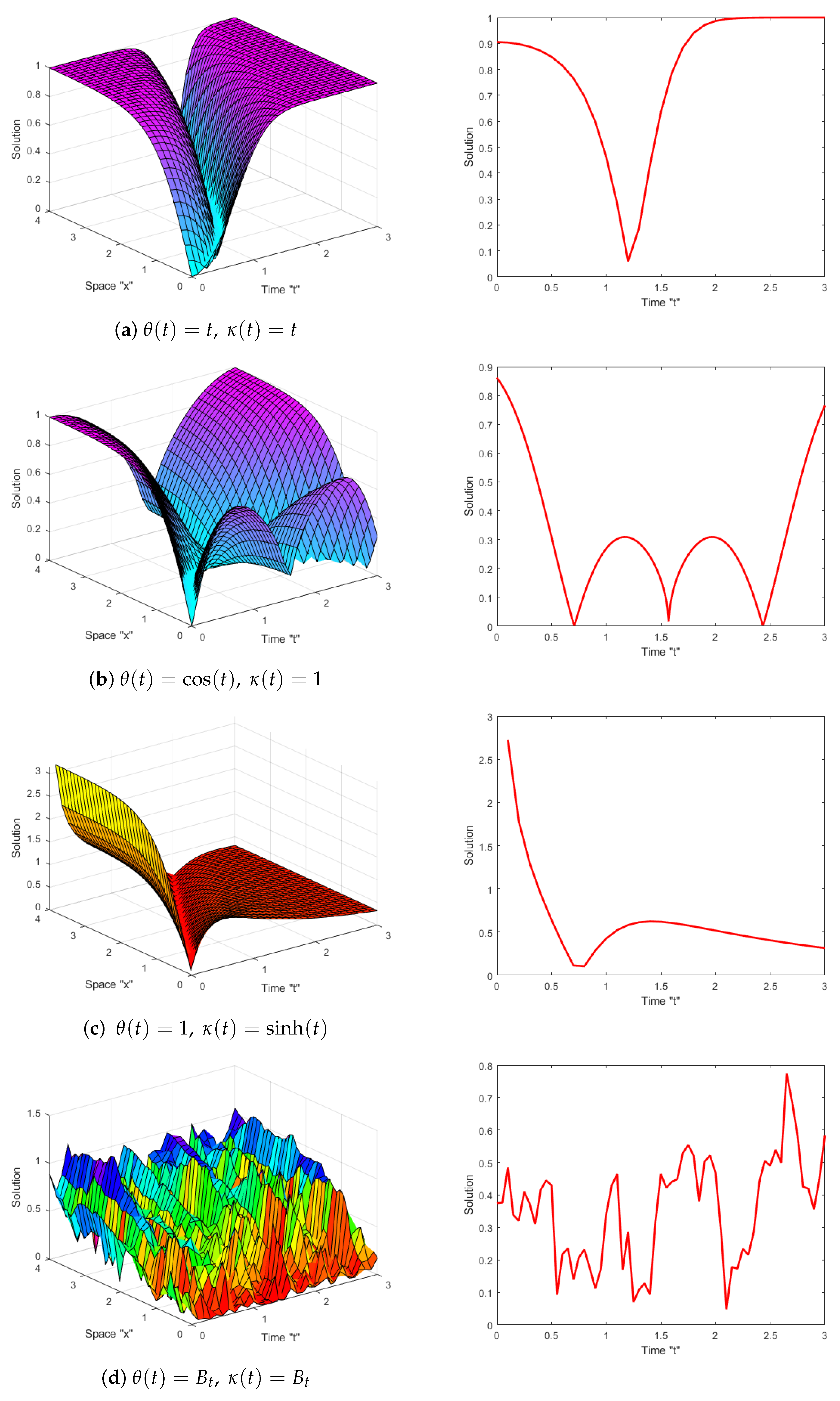
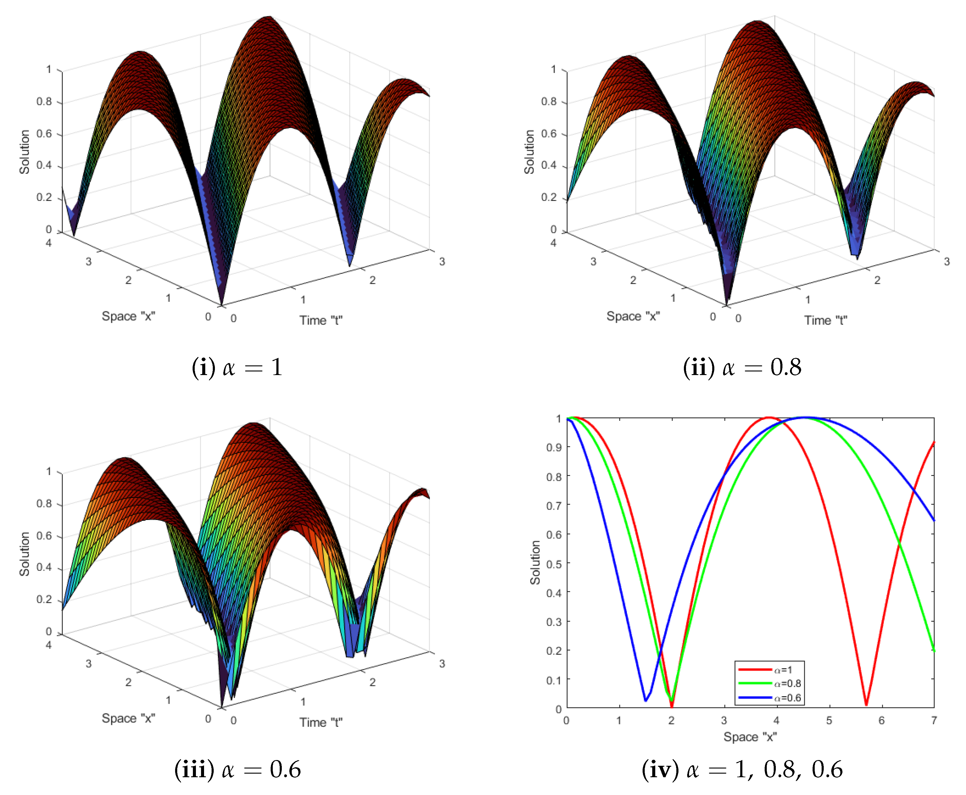
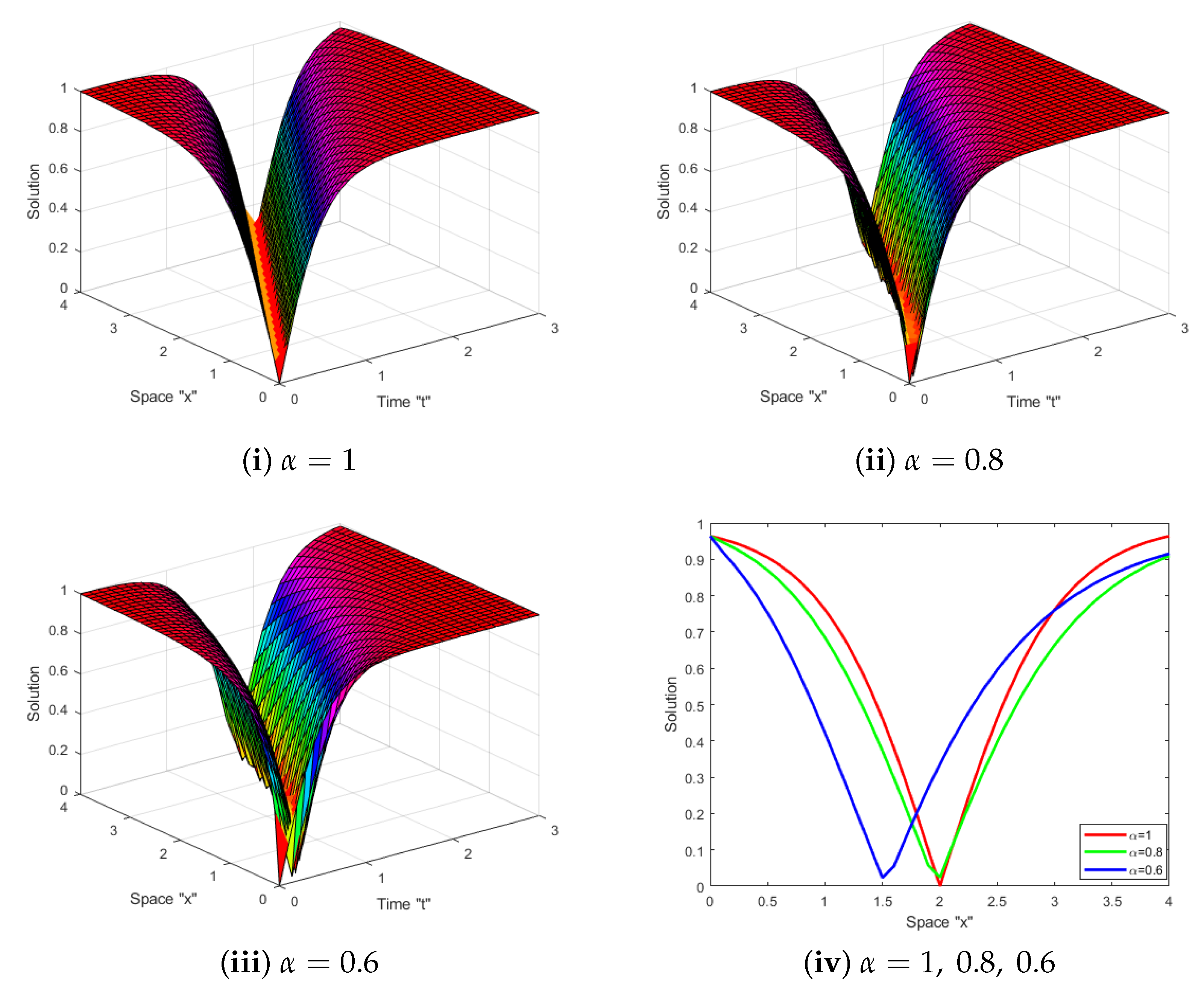
5. Effect of MTD and TDCs

Impacts of time-dependent coefficients: Now, the influence of the TDCs on the obtained solutions of the FSE-TDCs is discussed. Figure 1 and Figure 2 present the solutions $\left|\mathcal{U}(x,t)\right|$ stated in Equations (14) and (15) for $\mu =\rho =1,\delta =0,t\in [0,3],x\in [0,4]$ and $\alpha =1$. In Figure 1a and Figure 2a, we suppose $\kappa \left(t\right)=\theta \left(t\right)=t,$ and due to this selection, the surface twists from the left. In Figure 1b and Figure 2b, let $\theta \left(t\right)=cos\left(t\right)$ and $\kappa \left(t\right)=1,$ and this selection impacts on the sides of surface. In Figure 1c and Figure 2c, we suppose $\kappa \left(t\right)=sinh\left(t\right),$ and $\theta \left(t\right)=1;$ with this setting, the surface appears somewhat flat from the right. Whereas in Figure 1d and Figure 2d, let $\theta \left(t\right)=\kappa \left(t\right)=B_t\left(t\right),$ where $B\left(t\right)$ is the Brownian motion $B\left(t\right)$ and $B_t\left(t\right)={\displaystyle \frac{\partial B}{\partial t}}$; this setting makes the surface fluctuate.

Figure 1. Shows the 2D- and 3D-shapes for the solution $\left|\mathcal{U}(x,t)\right|$ given in Equation (14) with various TDCs.

Figure 2. Shows the 2D- and 3D-shapes for the solution $\left|\mathcal{U}(x,t)\right|$ given in Equation (15) with various TDCs.

Impacts of MTD: The influence of MTD on the obtained solutions of the FSE-TDCs (1) is now examined. The unknown variables are given appropriate values to create many two- and three-dimensional graphs. Behavior solutions for (14) and (15) are shown in Figure 3 and Figure 4. Figure 3 displays the periodic solutions $\left|\mathcal{U}(x,t)\right|$ indicated in Equation (14) for $\kappa \left(t\right)=\theta \left(t\right)=t,\mu =\rho =1,t\in [0,3],x\in [0,4],\delta =0.9$, and $\alpha =0.6,0.8,1$. Whereas Figure 4 shows the bright solutions $\left|\mathcal{U}(x,t)\right|$ indicated in Equation (15) for $\delta =0.9$, $\kappa \left(t\right)=\theta \left(t\right)=t,\mu =\rho =1,x\in [0,4],t\in [0,3]$, and for $\alpha =0.6,0.8,1$. These graphs show that the surface moves to the left when the derivative order $\alpha$ of MTD decreases.

Figure 3. (i–iii) exhibits the 3D-shape of the periodic solution $\left|\mathcal{U}(x,t)\right|,$ with $\alpha =1,0.8,0.6,$ given in Equation (14); (iv) presents the 2D-shape of Equation (14) with distinct $\alpha$.

Figure 4. (i–iii) show the 3D-shape of the bright solution $\left|\mathcal{U}(x,t)\right|,$ with $\alpha =0.6,0.8,1,$ given in Equation (15); (iv) presents the 2D-shape of Equation (15) with distinct $\alpha$.

Discussion: In this work, the solutions of the FSE-TDCs (1) were obtained. We applied two different methods including the mapping method and the $(G^{\prime }/G)$-expansion method. Solving the Schrödinger equation with time-dependent coefficients is crucial for understanding the behavior of quantum systems in non-equilibrium conditions. Many physical systems in nature are subject to time-varying external influences, such as electric and magnetic fields. By solving the time-dependent Schrödinger equation, researchers can predict how quantum systems will evolve over time and develop new insights into the dynamics of complex quantum phenomena.

6. Conclusions

The fractional Schrödinger equation with time-dependent coefficients (FSE-TDCs) was examined in this work. By using the mapping method and the $(G^{\prime }/G)$-expansion method, the exact solutions of FSE-TDCs were obtained. These approaches provide many types of solutions with parameters, including the dark optical solution, bright solutions, kink solutions, periodic solutions, the singular solution, and others. Because the Schrödinger equation is extensively used in quantum computing, quantum mechanics, physics, engineering, and chemistry, the generated solutions may be utilized to explore a wide range of important physical phenomena. We established several previous results, including those published in [24,25]. Furthermore, we addressed the impact of the coefficients, which have particular values, including random, polynomial, trigonometric, and hyperbolic functions, on the analytical solutions of FSE-TDCs (1). Also, we studied the effect of fractional-order derivatives on the obtained solutions. In future work, we can obtain the solutions of the Schrödinger Equation (1) when forced by additive noise. Also, we can use other functions, such as exponential, logarithmic, elliptical, and rational functions, to see how these functions impact on the solutions of (1).

References

- Oldham, K.B.; Spanier, J. The Fractional Calculus: Theory and Applications of Differentiation and Ntegration to Arbitrary Order; Mathematics in Science and Engineering; Academic Press: New York, NY, USA, 1974; Volume 11. [Google Scholar]
- Podlubny, I. Fractional Differential Equations; Mathematics in Science and Engineering; Academic Press: San Diego, CA, USA, 1999; Volume 198. [Google Scholar]
- Hilfer, R. Applications of Fractional Calculus in Physics; World Scientific Publishing: Singapore, 2000. [Google Scholar]
- Mohammed, W.W.; Cesarano, C.; Elsayed, E.M.; Al-Askar, F.M. The Analytical Fractional Solutions for Coupled Fokas System in Fiber Optics Using Different Methods. Fractal Fract. 2023, 7, 556. [Google Scholar] [CrossRef]
- Zeki, M.; Tinaztepe, R.; Tatar, S.; Ulusoy, S.; Al-Hajj, R. Determination of a Nonlinear Coefficient in a Time-Fractional Diffusion Equation. Fractal Fract. 2023, 7, 371. [Google Scholar] [CrossRef]
- Ismael, H.F.; Nabi, H.R.; Sulaiman, T.A.; Shah, N.A.; Ali, M.R. Multiple soliton and M-lump waves to a generalized B-type Kadomtsev–Petviashvili equation. Results Phys. 2023, 48, 106402. [Google Scholar] [CrossRef]
- Biswas, A. Solitary wave solution for KdV equation with power-law nonlinearity and time-dependent coefficients. Nonlinear Dyn. 2009, 58, 345–348. [Google Scholar] [CrossRef]
- Mohammed, W.W.; Iqbal, N.; Bourazza, S.; Elsayed, E.M. The optical structures for the fractional chiral nonlinear Schrödinger equation with time-dependent coefficients. Opt. Quantum Electron. 2024, 56, 1476. [Google Scholar] [CrossRef]
- Qi, J.; Zhu, Q. Further results about the non-traveling wave exact solutions of nonlinear Burgers equation with variable coefficients. Results Phys. 2023, 46, 106285. [Google Scholar] [CrossRef]
- Zayed, E.M.E.; Abdelaziz, M.A.M. Travelling wave solutions for the Burgers equation and the Korteweg-de Vries Equation with variable coefficients using the generalized (G′/G)-expansion method. Z. Naturforsch. 2010, 65, 1065–1070. [Google Scholar] [CrossRef]
- Injrou, S. Exact solutions for the Conformable space-time fractional Zeldovich equation with time-dependent coefficients. Int. J. Differ. Equ. 2022, 2020, 9312830. [Google Scholar] [CrossRef]
- Zhang, R.F.; Bilige, S.D. Bilinear neural network method to obtain the exact analytical solutions ofnonlinear partial differential equations and its application to p-gBKP equation. Nonlinear Dyn. 2019, 95, 3041–3048. [Google Scholar] [CrossRef]
- Qiao, J.M.; Zhang, R.F.; Yue, R.X.; Rezazadeh, H.; Seadawy, A.R. Three types of periodic solutions of new (3+1)-dimensional Boiti–Leon–Manna–Pempinelli equation via bilinear neuralnetwork method. Math. Methods Appl. Sci. 2022, 45, 5612–5621. [Google Scholar] [CrossRef]
- Wu, X.S.; Liu, J.G. Solving the variable coefficient nonlinear partial differential equations based on the bilinear residual network method. Nonlinear Dyn. 2024, 112, 8329–8340. [Google Scholar] [CrossRef]
- Zhang, R.F.; Li, M.C. Bilinear residual network method for solving the exactly explicit solutions of nonlinear evolution equations. Nonlinear Dyn. 2022, 108, 521–531. [Google Scholar] [CrossRef]
- Kuzenov, V.V.; Ryzhkov, S.V.; Varaksin, A.Y. Development of a method for solving elliptic differential equations based on a nonlinear compact-polynomial scheme. J. Comput. Appl. Math. 2024, 451, 116098. [Google Scholar] [CrossRef]
- De Bouard, A.; Debussche, A. A stochastic nonlinear Schrödinger equation with multiplicative noise. Commun. Math. Phys. 1999, 205, 161–181. [Google Scholar] [CrossRef]
- De Bouard, A.; Debussche, A. A semidiscrete scheme for the stochastic nonlinear Schrödinger equation. Numer. Math. 2004, 96, 733–770. [Google Scholar] [CrossRef]
- Grecksch, W.; Lisei, H. Stochastic nonlinear equations of Schrödinger type. Stoch. Anal. Appl. 2011, 29, 631–653. [Google Scholar] [CrossRef]
- Bruneau, C.H.; Di Menza, L.; Lehner, T. Numerical resolution of some nonlinear Schrödinger-like equations in plasmas. Numer. Meth. PDEs 1999, 15, 672–696. [Google Scholar] [CrossRef]
- Li, J.B. Exact dark soliton, periodic solutions and chaotic dynamics in a perturbed generalized nonlinear Schrödinger equation. Can. Appl. Math. Q. 2009, 17, 161–173. [Google Scholar]
- Tian, S.F. The mixed coupled nonlinear Schrödinger equation on the half-line via the Fokas method. Proc. R. Soc. Lond. A 2016, 472, 0588. [Google Scholar] [CrossRef]
- Zayed, E.M.; Shohib, R.M. Solitons and other solutions to the resonant nonlinear Schrödinger equation with both spatio-temporal and inter-modal dispersions using different techniques. Optik 2018, 158, 970–984. [Google Scholar] [CrossRef]
- Öziş, T.; Yıldırım, A. Application of He’s semi-inverse method to the nonlinear Schrödinger equation. Comput. Math. Appl. 2007, 54, 1039–1042. [Google Scholar] [CrossRef]
- Taghizadeh, N.; Mirzazadeh, M.; Farahrooz, F. Exact solutions of the nonlinear Schrödinger equation by the first integral method. J. Math. Anal. Appl. 2011, 374, 549–553. [Google Scholar] [CrossRef]
- Riesz, M. L’intégrale de Riemann-Liouville et le problème de Cauchy pour l’équation des ondes. Bull. Soc. Math. Fr. 1939, 67, 153–170. [Google Scholar] [CrossRef]
- Wang, K.L.; Liu, S.Y. He’s fractional derivative and its application for fractional Fornberg-Whitham equation. Therm. Sci. 2016, 1, 54. [Google Scholar] [CrossRef]
- Miller, S.; Ross, B. An Introduction to the Fractional Calculus and Fractional Differential Equations; Wiley: New York, NY, USA, 1993. [Google Scholar]
- Caputo, M.; Fabrizio, M. A new definition of fractional differential without singular kernel. Prog. Fract. Differ. Appl. 2015, 1, 1. [Google Scholar]
- Sousa, J.V.; de Oliveira, E.C. A new truncated Mfractional derivative type unifying some fractional derivative types with classical properties. Int. J. Anal. Appl. 2018, 16, 83–96. [Google Scholar]
- Bhrawy, A.H.; Abdelkawy, M.A.; Kumar, S.; Johnson, S.; Biswas, A. Solitons and other solutions to quantum Zakharov–Kuznetsov equation in quantum magneto-plasmas. Indian J. Phys. 2013, 87, 455–463. [Google Scholar] [CrossRef]
- Wang, M.L.; Li, X.Z.; Zhang, J.L. The (G′/G)-expansion method and travelling wave solutions of nonlinear evolution equations in mathematical physics. Phys. Lett. A 2008, 372, 417–423. [Google Scholar] [CrossRef]
Disclaimer/Publisher’s Note: The statements, opinions and data contained in all publications are solely those of the individual author(s) and contributor(s) and not of MDPI and/or the editor(s). MDPI and/or the editor(s) disclaim responsibility for any injury to people or property resulting from any ideas, methods, instructions or products referred to in the content. |
© 2025 by the authors. Licensee MDPI, Basel, Switzerland. This article is an open access article distributed under the terms and conditions of the Creative Commons Attribution (CC BY) license (https://creativecommons.org/licenses/by/4.0/).