


Fractal Analysis of Volcanic Rock Image Based on Difference Box-Counting Dimension and Gray-Level Co-Occurrence Matrix: A Case Study in the Liaohe Basin, China


Abstract
1. Introduction
1.1. The Theoretical Basis of Volcanic Rock Lithology Identification
1.2. Comparison of Advantages Between Traditional Methods and Fractal Dimension
1.3. Fractal Geometry
1.4. Gray Release Co-Occurrence Matrix
1.5. DBC-GLCM
2. Samples and Methods
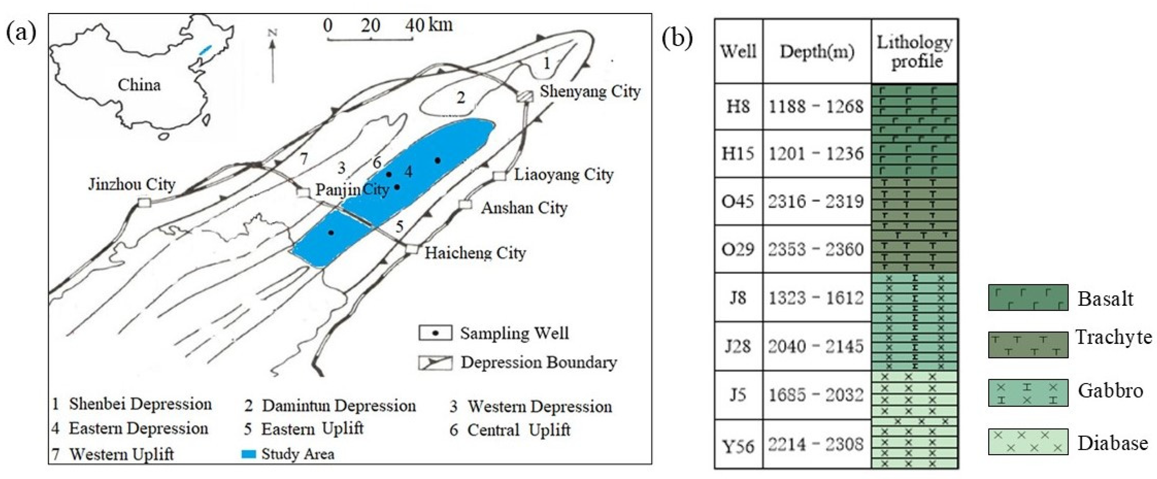
2.1. Geological Background and Samples
2.2. Experimental Data Preprocessing
2.2.1. Image Gray Release
2.2.2. Filtering Processing
- (1)
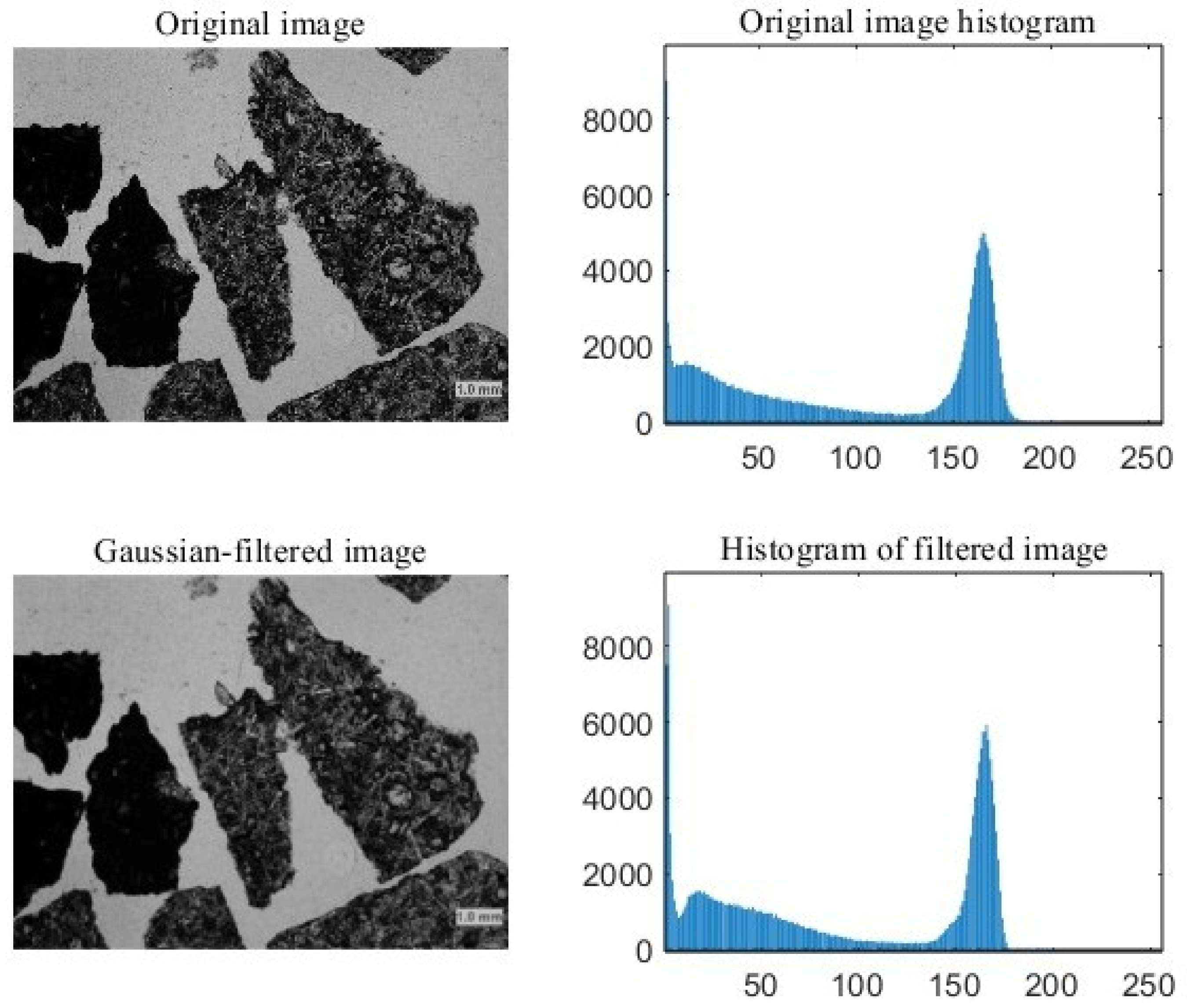
- Gaussian filtering: It belongs to linear smoothing filtering. The principle is to perform a weighted average on the image. The value of each pixel is obtained by a weighted average of its own value and those of other pixels in the neighborhood. Figure 3 shows the result of Gaussian filtering.
- (2)
- Median filtering: It is a type of non-linear filtering. Its principle is to replace the grayscale value of a pixel with the median value of the grayscale values in the neighborhood of that pixel. The advantage of this method is that the obtained pixel values are mostly real values, and isolated noise points can be easily removed. Figure 4 shows the result of median filtering.
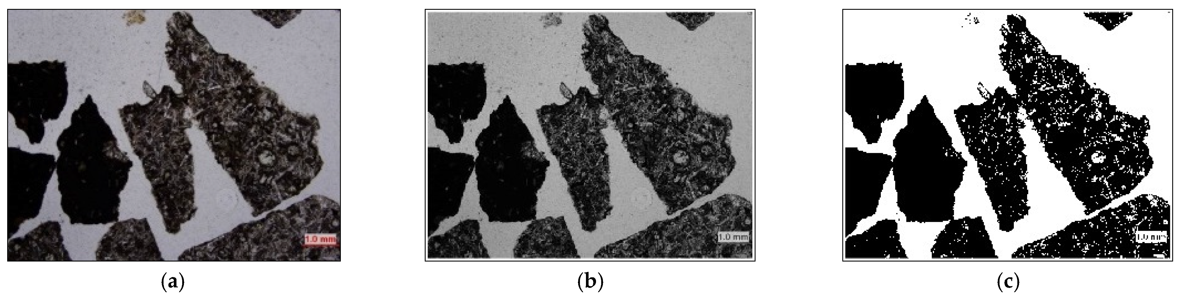
2.2.3. Binarization
2.3. Methods
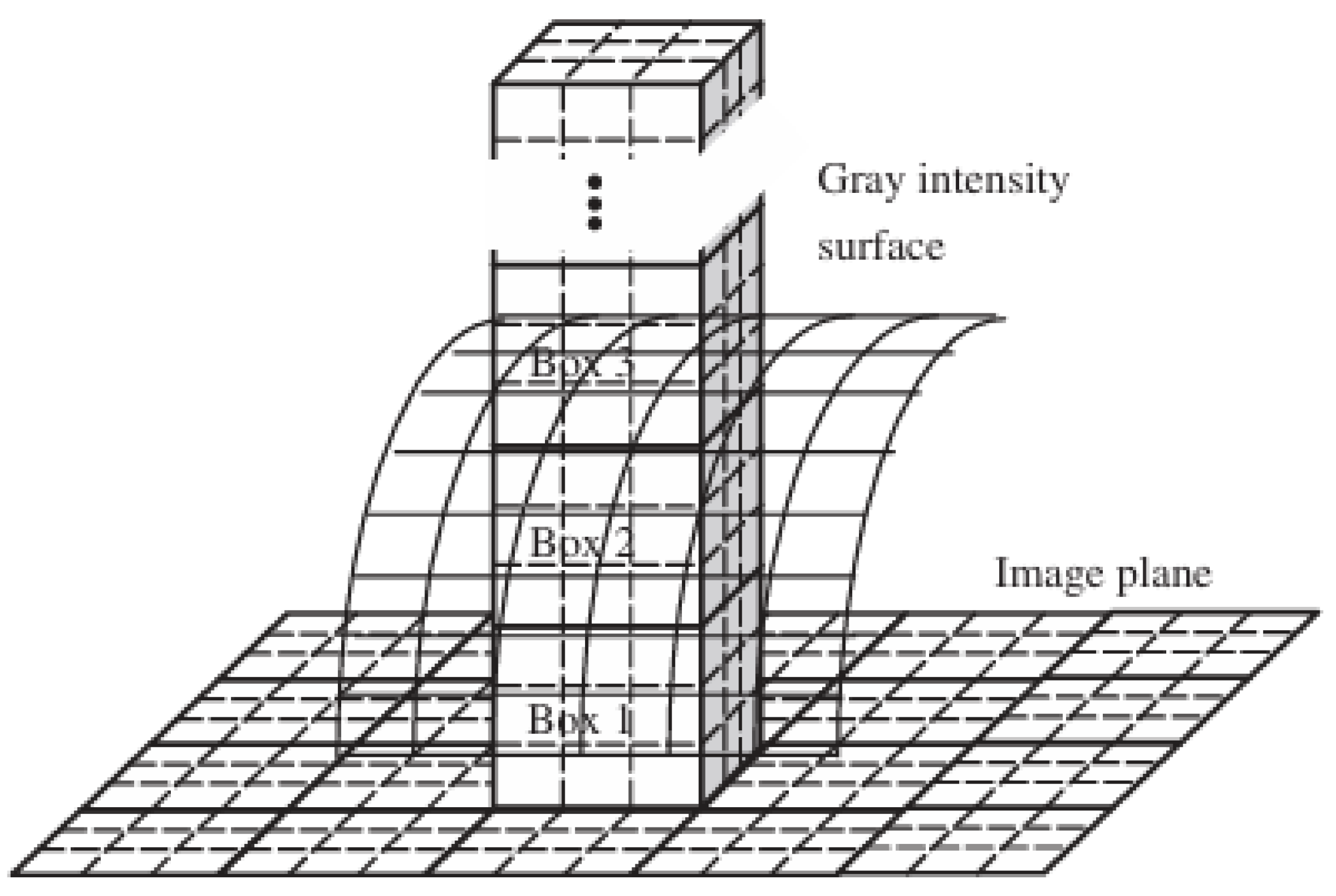
2.3.1. DBC
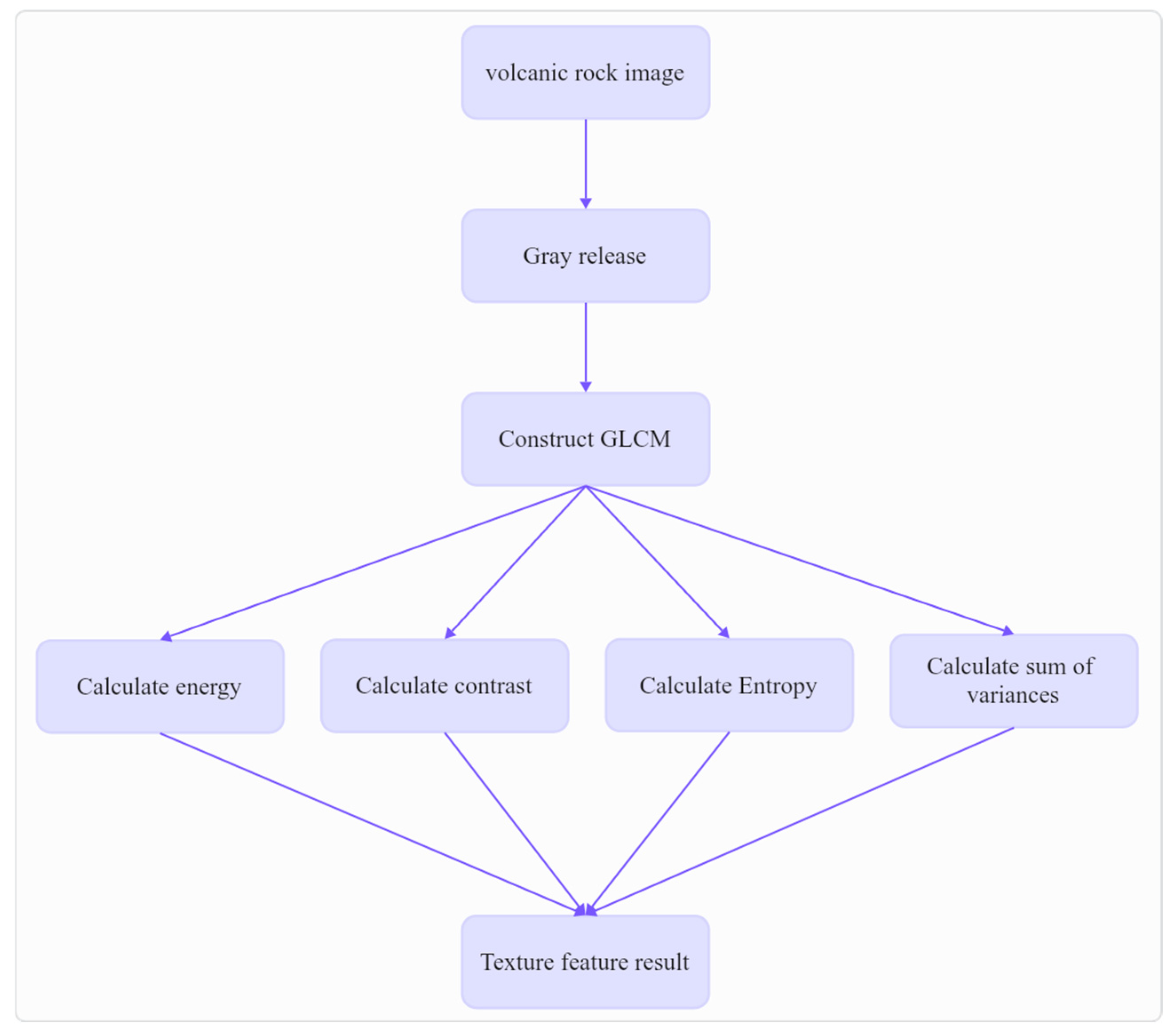
2.3.2. GLCM
- Contrast : Contrast is manifested by the difference in brightness of pixel points in image textures. It is related to the gray values and positions of pixels and reflects the amplitude of local grayscale changes in an image.
- Energy : Energy, also known as angular second moment, is the sum of the squares of all elements in the gray-level co-occurrence matrix. It can reflect the uniformity of the gray distribution and the coarseness or fineness of the texture in an image.
- Entropy : Entropy represents the amount of information in an image and can characterize the complexity of textures. It reflects the randomness or complexity of textures in an image. The greater the entropy value is, the more complex the texture will be.
- Sum of variances : Among them, m is the mean value of p.
- Sum of averages : The mean value sum is a measure of the average gray value of the pixel points within the image area, reflecting the brightness and darkness of the image and is applicable to grayscale images.
3. Results
3.1. DBC Experiment Results
- As can be seen from Figure 12, the difference box-counting dimension of volcanic rocks in this area ranges from 1.6 to 1.9. The surface texture of volcanic rocks is relatively complex, and its difference box-counting dimension is between 1 and 2 (the difference box-counting dimension of a straight line is 1, and that of a planar figure is 2).
- The difference box-counting dimensions of trachyte, diabase, and gabbro are all larger than that of basalt, indicating that the surface structures of trachyte, diabase, and gabbro are more complex than that of basalt. As can be seen from the obtained data, the differential box-counting dimension can, to a certain extent, distinguish basalt and trachyte from the other two types of volcanic rocks. When the fractal dimension ranges of diabase and gabbro overlap (1.76–1.84), the FD-GLCM method is comprehensively utilized to distinguish the lithologies of these three types of volcanic rocks.
3.2. GLCM Experiment Results
4. Discussion
4.1. Model Evaluation
4.2. Analysis of Application Effect
4.3. Computational Complexity of DBC and GLCM Methods
4.4. Limitation
4.5. Practical Application and Scalability
5. Conclusions
- (1)
- The images of volcanic rocks indicate that the microscopic structures of volcanic rocks are fractal structures with self-similarity, the complexity of which can be described by the magnitude of the fractal dimension. The value of the differential box-counting dimension of volcanic rocks is in direct proportion to the complexity of the rock surface. For rocks with more complex surface textures, the calculated values of the differential box-counting dimension will be larger.
- (2)
- The differential box-counting dimension of basalt ranges from 1.7 to 1.75, that of trachyte ranges from 1.82 to 1.87, that of gabbro ranges from 1.76 to 1.79, and that of diabase ranges from 1.78 to 1.82. The application of the differential box-counting dimension can distinguish basalt from the other three types of volcanic rocks.
- (3)
- Since the differential box-counting dimensions of trachyte, diabase, and gabbro overlap to some extent, we further comprehensively utilize the differential box-counting dimension and the gray-level co-occurrence matrix method to distinguish the lithology of volcanic rocks. In terms of the W3 value, it is gabbro when W3 > 14 and diabase when W3 < 14. Compared with the method of identifying volcanic rocks based on a single feature, the method that combines the differential box-counting dimension and the gray-level co-occurrence matrix is more accurate in identifying the lithology of volcanic rocks.
Author Contributions
Funding
Data Availability Statement
Conflicts of Interest
References
- Zou, C.-N.; Zhao, W.-Z.; Jia, C.-Z.; Zhu, R.-K.; Zhang, G.-Y.; Zhao, X.; Yuan, X.-J. Formation and distribution of volcanic hydrocarbon reservoirs in sedimentary basins of China. Pet. Explor. Dev. 2008, 3, 257–271. [Google Scholar] [CrossRef]
- Liu, B.; Zhang, B.; Guo, Q.; Tan, N.; Wang, J.; Chen, X. Discovery and exploration inspiration of deep volcanic gas reservoirs in eastern sag of Liaohe depression. China Pet. Explor. 2020, 25, 33–43. [Google Scholar]
- He, H.; Li, S.; Liu, C.; Kong, C.; Jiang, Q.; Chang, T. Characteristics and quantitative evaluation of volcanic effective reservoirs: A case study from Junggar Basin, China. J. Pet. Sci. Eng. 2020, 195, 107723. [Google Scholar] [CrossRef]
- Hu, C.; Deng, Q.; Lin, L.; Hu, M.; Hou, X.; Zong, L.; Song, P.; Kane, O.I.; Cai, Q.; Hu, Z. Lower Cretaceous volcanic-sedimentary successions of the continental rift basin in the Songliao Basin, northeast China: Implication in high-quality reservoir prediction and hydrocarbon potential. Mar. Pet. Geol. 2023, 158, 106540. [Google Scholar] [CrossRef]
- Fan, C.; Li, H.; Qin, Q.; Shang, L.; Yuan, Y.; Li, Z. Formation Mechanisms and Distribution of Weathered Volcanic Reservoirs: A Case Study of the Carboniferous Volcanic Rocks in Northwest Junggar Basin, China. Energy Sci. Eng. 2020, 8, 8. [Google Scholar] [CrossRef]
- Kousehlar, M.; Weisenberger, T.; Tutti, F.; Mirnejad, H. Fluid Control on Low-temperature Mineral Formation in Volcanic Rocks of Kahrizak, Iran. Geofluids 2012, 12, 295–311. [Google Scholar] [CrossRef]
- Dong, S.; Wang, Z.; Zeng, L. Lithology identification using Kernel Fisher discriminant analysis with well logs. J. Pet. Sci. Eng. 2016, 143, 95–102. [Google Scholar] [CrossRef]
- Xu, T.; Chang, J.; Feng, D.; Lv, W.; Kang, Y.; Liu, H.; Li, J.; Li, Z. Evaluation of active learning algorithms for formation lithology identification. J. Pet. Sci. Eng. 2021, 206, 108999. [Google Scholar] [CrossRef]
- Duan, Y.; Xie, J.; Su, Y.; Liang, H.; Hu, X.; Wang, Q.; Pan, Z. Application of the decision three method to lithology identification of volcanic rocks-taking the Mesozoic in the Laizhouwan Sag as an example. Sci. Rep. 2020, 11, 19209. [Google Scholar]
- Lyu, Q.; Luo, S.; Guan, Y.; Fu, J.; Niu, X.; Xu, L.; Feng, S.; Li, S. A New Method of Lithologic Identification and Distribution Characteristics of Fine—Grained Sediments: A Case Study in Southwest of Ordos Basin, China. Open Geosci. 2019, 26, 17–28. [Google Scholar] [CrossRef]
- Xu, Z.; Shi, H.; Lin, P.; Liu, T. Integrated lithology identification based on images and elemental data from rocks. J. Pet. Sci. Eng. 2021, 205, 108853. [Google Scholar] [CrossRef]
- Lai, J.; Fan, X.; Liu, B.; Pang, X.; Zhu, S.; Xie, W.; Wang, G. Qualitative and quantitative prediction of diagenetic facies via well logs. Mar. Pet. Geol. 2020, 120, 104486. [Google Scholar] [CrossRef]
- Shehata, A.A.; Osman, O.A.; Nabawy, B.S. Neural network application to petrophysical and lithofacies analysis based on multi-scale data: An integrated study using conventional well log, core and borehole image data. J. Nat. Gas Sci. Eng. 2021, 93, 104015. [Google Scholar] [CrossRef]
- Mandelbrot, B.; Passoja, D.; Paullay, A. Fractal character of fracture surfaces of metal. Nature 1984, 308, 721–722. [Google Scholar] [CrossRef]
- Pentland, A.P. Fractal-based description of natural scenes. IEEE Trans. Pattern Anal. Mach. Intell. 1984, 6, 661–674. [Google Scholar] [CrossRef]
- Peleg, S.; Naor, J.; Hartley, R.; Avnir, D. Multiple resolution texture analysis and classification. IEEE Trans. Pattern Anal. Mach. Intell. 1984, 4, 518–523. [Google Scholar] [CrossRef]
- Sarkar, N.; Chaudhuri, B.B. An efficient differential box-counting approach to compute fractal dimension of image. IEEE Trans. Syst. Man Cybern. 1994, 24, 115–120. [Google Scholar] [CrossRef]
- Leary Peter, C. Deep borehole log evidence for fractal distribution of fractures in crystalline rock. Geophys. J. Int. 1991, 107, 615. [Google Scholar] [CrossRef]
- Jorge, L.; Luis, O.; Jerson, G. Identification of Natural Fractures using Resistive Image Logs, Fractal Dimension and Support Vector Machines. Ing. E Investig. 2016, 36, 125. [Google Scholar]
- Peng, R.; Yang, Y.; Ju, Y.; Mao, L.; Yang, Y. Computation of Fractal Dimension of Rock Pores Based on Gray CT Images. Chin. Sci. Bull. 2011, 56, 2256–2266. [Google Scholar] [CrossRef]
- Xia, Y.; Cai, J.; Perfect, E.; Wei, W.; Zhang, Q.; Meng, Q. Fractal Dimension, Lacunarity and Succolarity Analyses on CT Images of Reservoir Rocks for Permeability Prediction. J. Hydrol. 2019, 579, 124198. [Google Scholar] [CrossRef]
- Haralick, R.M.; Shanmugam, K.; Dinstein, I. Textural features for image classification. IEEE Trans. Syst. Man Cybern. 1973, SMC-3, 610–621. [Google Scholar] [CrossRef]
- Haralick, R.M. Statistical and structural approaches to texture. Proc. IEEE 1979, 67, 786–804. [Google Scholar] [CrossRef]
- Garg, M.; Dhiman, G. A novel content-based image retrieval approach for classification using GLCM features and texture fused LBP variants. Neural Comput. Appl. 2020, 33, 1311–1328. [Google Scholar] [CrossRef]
- Singh, A.; Armstrong, R.T.; Regenauer-Lieb, K.; Mostaghimi, P. Rock characterization using gray-level co-occurrence matrix: An objective perspective of digital rock statistics. Water Resour. Res. 2019, 55, 1912–1927. [Google Scholar] [CrossRef]
- Xie, Y.; Wang, J. Study on the identification of the wood surface defects based on texture features. Optik 2015, 126, 2231–2235. [Google Scholar]
- Saptarshi, C.; Debangshu, D.; Sugata, M. Integration of morphological preprocessing and fractal based feature extraction with recursive feature elimination for skin lesion types classification. Comput. Methods Programs Biomed. 2019, 178, 201–218. [Google Scholar]
- Peng, W.; Hu, G.; Feng, Z.; Liu, D.; Wang, Y.; Lv, Y.; Zhao, R. Origin of Paleogene Natural gases and discussion of abnormal carbon isotopic composition of heavy alkanes in the Liaohe Basin, NE China. Mar. Pet. Geol. 2018, 92, 670–684. [Google Scholar] [CrossRef]
- Huang, S.; Feng, Z.; Gu, T.; Gong, D.; Peng, W.; Yuan, M. Multiple origins of the Paleogene natural gases and effects of secondary alteration in Liaohe Basin northeast China: Insights from the molecular and stable isotopic compositions. Int. J. Coal Geol. 2017, 172, 134–148. [Google Scholar] [CrossRef]
- Li, S.; Huang, Y.; Feng, Y.; Guo, Y.; Zhang, B.; Wang, P. Cenozoic extension and strike-slip tectonics and fault structures in the eastern sag, Liaohe depression. Chin. J. Geophys.-Chin. Ed. 2020, 63, 612–626. [Google Scholar]
- Han, R.; Wang, Z.; Wang, W.; Xu, F.; Qi, X.; Cui, Y.; Zhang, Z. Igneous rocks lithology identification with deep forest: Case study from eastern sag, Liaohe Basin. J. Appl. Geophys. 2023, 208, 104892. [Google Scholar] [CrossRef]
- Wang, W.; Lin, C.; Zhang, X. Fractal dimension analysis of pore throat structure in tight sandstone reservoirs of Huagang formation: Jiaxing area of east China sea basin. Fractal Fract. 2024, 8, 374. [Google Scholar] [CrossRef]
- Asawari, K.; Aparna, J. Gray-scale image compression technique: A review. Int. J. Comput. Appl. 2015, 131, 22–25. [Google Scholar]
- Saha, S.K.; Pradhan, S.; Barai, S.V. Use of machine learning based technique to X-ray microtomographic images of concrete for phase segmentation at meso-scale. Constr. Build. Mater. 2020, 249, 118744. [Google Scholar] [CrossRef]
- Sherzer, G.L.; Alghalandis, Y.F.; Peterson, K.; Shah, S. Comparative study of scale effect in concrete fracturing via Lattice Discrete Particle and Finite Discrete Element Models. Eng. Fail. Anal. 2022, 135, 106062. [Google Scholar] [CrossRef]
- Gencel, O.; Nodehi, M.; Bozkurt, A.; Sarı, A.; Ozbakkaloglu, T. The use of computerized tomography (CT) and image processing for evaluation of the properties of foam concrete produced with different content of foaming agent and aggregate. Constr. Build. Mater. 2023, 399, 132433. [Google Scholar] [CrossRef]
- Yoon, J.; Kim, H.; Sim, S.-H.; Pyo, S. Characterization of porous cementitious materials using microscopic image processing and X-ray CT analysis. Materials 2020, 13, 3105. [Google Scholar] [CrossRef]
- Sherzer, G.L.; Alghalandis, Y.F.; Peterson, K. Introducing fracturing through aggregates in LDPM. Eng. Fract. Mech. 2022, 261, 108228. [Google Scholar] [CrossRef]
- Li, J.; Du, Q.; Sun, C. An improved box-counting method for image fractal dimension estimation. Pattern Recognit. 2009, 42, 2460–2469. [Google Scholar] [CrossRef]
- Chinmaya, P.; Ayan, S.; Nihar, K.M.; Debotosh, B. Differential box counting methods for estimating fractal dimension of gray-scale images: A survey. Chaos Solitons Fractals 2019, 126, 178–202. [Google Scholar]
- Cristina, M.; Laura, F.; Riccardo, G.; Ernestina, C.; Riccardo, R. Glcm, an image analysis technique for early detection of biofilm. J. Eng. 2016, 185, 48–55. [Google Scholar]
- Gabriel, R.G.; Gabriel, P.; Alejandro, P.; Alejandro, C.; Cristina, W.; Samanta, S.S.; Emilia, L.; Nieves, P. Assessment of multi-data sentinel-1 polarizations and GLCM texture features capacity for onion and sunflower classification in an irrigated valley: An object level approach. Agronomy 2020, 10, 845. [Google Scholar]
- Paladugu, R.; Veera, M.R.; Bhima, P.R. Optimal GLCM combined FCM segmentation algorithm for detection of kidney cysts and tumor. Multimed. Tools Appl. 2019, 78, 18419–18441. [Google Scholar]
- Redouan, K.; Sidi, M.F.; Abderrahmane, S.; Rajaa, T.; Mustapha, T. A combined method of fractal and GLCM features for MRI and CT scan images classification. Signal Image Process. 2014, 5, 4. [Google Scholar]


| d | W1 | W2 (1 × 10⁻⁴) | W3 | W4 | W5 |
|---|---|---|---|---|---|
| d = 1 | 18,575.288 | 4.115 | 13.231 | 123.162 | 3406.308 |
| d = 2 | 18,550.121 | 3.279 | 13.615 | 123.061 | 3406.229 |
| d = 3 | 18,526.246 | 3.006 | 13.759 | 122.965 | 3405.892 |
| d = 4 | 18,505.105 | 2.821 | 13.847 | 122.871 | 3405.526 |
| d | W1 | W2 (1 × 10⁻⁴) | W3 | W4 | W5 |
|---|---|---|---|---|---|
| d = 1 | 32,059.146 | 2.461 | 13.657 | 169.219 | 3423.735 |
| d = 2 | 32,035.065 | 1.892 | 13.962 | 169.144 | 3425.269 |
| d = 3 | 32,014.594 | 1.787 | 14.057 | 169.078 | 3427.228 |
| d = 4 | 31,994.295 | 1.702 | 14.119 | 169.013 | 3428.788 |
| Sample | W1 | W2 (1 × 10⁻⁴) | W3 | W4 | W5 |
|---|---|---|---|---|---|
| 1 | 18,597.376 | 4.959 | 13.092 | 3406.319 | 123.252 |
| 2 | 21,326.265 | 5.118 | 12.873 | 2851.409 | 135.922 |
| 3 | 18,911.328 | 1.212 | 13.948 | 2696.592 | 127.337 |
| 4 | 18,453.301 | 1.553 | 13.612 | 2978.959 | 124.396 |
| 5 | 17,703.911 | 6.291 | 12.773 | 4230.387 | 116.075 |
| 6 | 13,253.303 | 1.706 | 13.778 | 3667.949 | 97.905 |
| 7 | 23,534.587 | 4.499 | 12.618 | 2156.852 | 146.211 |
| 8 | 27,924.793 | 9.424 | 11.761 | 1865.669 | 161.428 |
| 9 | 18,904.292 | 6.849 | 12.361 | 4359.485 | 120.601 |
| 10 | 25,812.256 | 4.467 | 12.925 | 2061.523 | 154.114 |
| Sample | W1 | W2 (1 × 10⁻⁴) | W3 | W4 | W5 |
|---|---|---|---|---|---|
| 1 | 32,045.486 | 2.865 | 13.627 | 3424.492 | 169.1774 |
| 2 | 29,986.944 | 0.827 | 14.209 | 2795.745 | 164.898 |
| 3 | 20,582.479 | 0.949 | 13.836 | 2206.793 | 135.557 |
| 4 | 19,231.518 | 1.119 | 13.601 | 1848.355 | 131.845 |
| 5 | 26,672.479 | 1.586 | 14.188 | 4477.683 | 148.979 |
| 6 | 25,713.986 | 3.138 | 13.634 | 2599.351 | 152.035 |
| 7 | 22,705.355 | 1.158 | 13.653 | 2586.818 | 141.8398 |
| 8 | 20,343.634 | 1.849 | 13.509 | 1571.144 | 137.013 |
| 9 | 19,205.051 | 6.55 | 12.634 | 1972.271 | 131.274 |
| 10 | 22,749.615 | 5.87 | 12.083 | 5925.378 | 132.083 |
| Lithology | Random Forest Model | FD-GLCM | ||||
|---|---|---|---|---|---|---|
| Precision/1 | Recall/1 | F1 | Precision/1 | Recall/1 | F1 | |
| Basalt | 0.81 | 0.91 | 0.85 | 0.91 | 0.92 | 0.915 |
| Trachyte | 0.87 | 0.92 | 0.894 | 0.88 | 0.90 | 0.89 |
| Gabbro | 0.82 | 0.67 | 0.738 | 0.67 | 0.67 | 0.67 |
| Diabase | 0.76 | 0.67 | 0.712 | 0.87 | 0.78 | 0.823 |
| Accuracy/1 | 0.88 | 0.86 | ||||
Disclaimer/Publisher’s Note: The statements, opinions and data contained in all publications are solely those of the individual author(s) and contributor(s) and not of MDPI and/or the editor(s). MDPI and/or the editor(s) disclaim responsibility for any injury to people or property resulting from any ideas, methods, instructions or products referred to in the content. |
© 2025 by the authors. Licensee MDPI, Basel, Switzerland. This article is an open access article distributed under the terms and conditions of the Creative Commons Attribution (CC BY) license (https://creativecommons.org/licenses/by/4.0/).
Share and Cite
Li, S.; Wang, Z.; Mou, D. Fractal Analysis of Volcanic Rock Image Based on Difference Box-Counting Dimension and Gray-Level Co-Occurrence Matrix: A Case Study in the Liaohe Basin, China. Fractal Fract. 2025, 9, 99. https://doi.org/10.3390/fractalfract9020099
Li S, Wang Z, Mou D. Fractal Analysis of Volcanic Rock Image Based on Difference Box-Counting Dimension and Gray-Level Co-Occurrence Matrix: A Case Study in the Liaohe Basin, China. Fractal and Fractional. 2025; 9(2):99. https://doi.org/10.3390/fractalfract9020099
Chicago/Turabian StyleLi, Sijia, Zhuwen Wang, and Dan Mou. 2025. "Fractal Analysis of Volcanic Rock Image Based on Difference Box-Counting Dimension and Gray-Level Co-Occurrence Matrix: A Case Study in the Liaohe Basin, China" Fractal and Fractional 9, no. 2: 99. https://doi.org/10.3390/fractalfract9020099
APA StyleLi, S., Wang, Z., & Mou, D. (2025). Fractal Analysis of Volcanic Rock Image Based on Difference Box-Counting Dimension and Gray-Level Co-Occurrence Matrix: A Case Study in the Liaohe Basin, China. Fractal and Fractional, 9(2), 99. https://doi.org/10.3390/fractalfract9020099