The Adaptive Backstepping Synchronization Control for a Kind of Variable-Order Fractional Uncertain Nonlinear Systems

Abstract

This paper is concerned with the adaptive backstepping synchronization control for a class of variable-order (VO) fractional uncertain nonlinear system with external disturbances and a dead zone. A kind of VO fractional command filter is employed to cope with “explosion of complexity”. The unknown nonlinear term in considered system is decomposed into unknown parameters and error functions by the Szász–Mirakyan operator theory. A VO fractional disturbance observer derived in this paper is used to simultaneously deal with the difficulties brought by dead zone and external disturbances. Thus, a VO fractional backstepping synchronization controller with adaptive laws for the system handled is proposed; moreover, the stability of system controlled is established. Finally, numerical examples are given to validate the theoretical results.

1. Introduction

Roughly speaking, the fractional calculus consists of constant order (CO) fractional calculus and VO fractional calculus, with respect to the theory and application of CO fractional calculus, one can refer to the Refs. [1,2,3] and the references therein. Compared with CO fractional operator, the VO fractional operator established by Samko and Ross [4] can be used to describe more actual and complex systems due to its advantage at describing the memory properties of changes in time or spatial position, which results in that VO fractional operator possesses some unique properties, such as irreversibility of the VO fractional integration and differentiation, the violation of the law of exponents. For example, the following does not generally hold:

$$D^{q_1\left(t\right)+q_2\left(t\right)}x\left(t\right)=D^{q_1\left(t\right)}\left(D^{q_2\left(t\right)}x\left(t\right)\right),\forall q_1\left(t\right)\ge 0,q_2\left(t\right)\ge 0,$$

where $D^{q\left(t\right)}$ denotes the fractional derivative in some sense, to name but a few. Thus, the investigations on theory and applications including the control problems of VO fractional system are not just simple developments from CO fractional circumstances (for more detail, see Refs. [5,6,7,8,9]).

Backstepping control (BSC) method [10] is widely utilized to deal with the control problems for differential system. In the process of designing controller by BSC method, firstly, a complex nonlinear system is decomposed into subsystems that do not exceed the end of the system; then, a Lyapunov function and virtual control are designed for each subsystem; finally, the actual controller is designed for the last subsystem. It is mentioned that the Lyapunov functions and controllers invoked in BSC method are systematized and structured by reversing design. Moreover, the constraints in which the uncertainty acts as a matching condition in system considered are eliminated. However, the repeated derivative for the virtual control function in BSC method leads to increase the computational complexity which is referred as “explosion of complexity”. The command filter [11] which can generate the approximate signal of derivative for the virtual control function without the process of differentiation can be employed to overcome such obstacle. Nevertheless, when the order of system is high, the error generated by the command filter cannot be properly handled, such accumulating error would affect the performance and stability of the controlled system. The error compensation mechanism which is introduced by Ma et al. [12] can be employed to overcome such obstacle.

From the engineering standpoint, some inherent laws in mathematical modeling can only be described by unknown functions. The Szász–Mirakyan operator which is a type of Bernstein polynomial can be applied to approximate any unknown function. Compared with fuzzy logic systems which is a traditional method to deal with the unknown function, the approximation for unknown function which is produced by the Szász–Mirakyan operator theory is with a simple and effective form. Obviously, it can reduce the complexity in designing control process. By employing the Szász–Mirakyan operators, the robust control problem for CO fractional nonlinear uncertain systems with input time delay was considered in Ref. [13]. Invoking the Szász–Mirakyan operator theory, Izadbakhsh et al. [14] studied the impedance control problem for robot manipulators. In Ref. [15], the Szász–Mirakyan operator was utilized to estimate uncertain terms in the chaotic signals of the master and slave system.

In control science, a dead zone is a kind of input nonlinearity which leads to zero output; thus, a dead zone would bring negative effects on system stability. Combining the modeling of the dead zone by a bounded nonlinear transformation with some compensating method, Mei et al. [16] handled the event-triggered adaptive control for a kind of nonlinear systems with dead zone. Dong et al. [17] employed the Nussbaum function to effectively address the experience output dead zone problem which arise in the attitude control for multi-rotor unmanned aerial vehicles. During the designing process of controller for an uncertain strict-feedback nonlinear system with output constraints and dead zone, Ni and Shi [18] utilized the dead zone inverse technique to derive the actual control input. The bounded information of dead zone input slopes is frequently used to tackle obstacles brought by the dead zone and ensures the stability of the synchronization error system, for more detail, see Ref. [19]. The method proposed in Ref. [20] models the bounded component of the unknown dead zone along with external disturbances as a single composite disturbance.

In Ref. [21], the synchronization of CO fractional chaotic system with unknown functions was considered by using the adaptive fuzzy BSC method and command filter. Combining the BSC method with the adaptive finite time sliding mode control method, Xue et al. [22] studied the control problem for CO fractional nonlinear systems with actuator faults. As for the fuzzy synchronization for CO fractional chaotic systems, the investigation which relies on BSC approach with finite-time command filter is due to Alassafi et al. [23], in which the error compensation signals are invoked to eliminate the filtering approximation errors. Ye and Song [24] studied the control problem for high-order strict-feedback system by BSC method. It is mentioned that, with the help of time varying gain command filter, the complexity of control algorithms proposed in the literature [24] can be reduced. In order to deal with the synchronization control for uncertain CO fractional chaotic system with disturbances and partially unmeasurable states by BSC method with low complexity and low errors, Dong, Cao, and Liu [25] introduced the CO fractional command filter with an error compensation mechanism.

As indicated in the first paragraph of this section, the investigations on synchronization control problem of VO fractional system are not the simple developments from CO fractional circumstances; thus, this paper is dedicated to consider the synchronization control problem of VO fractional systems with external disturbances and dead zone. The contributions of this work are listed as follows:

• VO fractional command filter is developed to overcome the “explosion of complexity”in the process of designing controller by following BSC method, and an error compensation mechanism is introduced to compensate the inaccuracies arising from using command filter.
• Compared with the results in [21,26,27,28,29] which considered the unknown function by fuzzy logic system, combining the Szász–Mirakyan operator with adaptive law, which is invoked in our paper, is a simple and effective method to deal with the difficulties brought by unknown functions.
• VO fractional disturbance observer is designed to cope with the unknown external disturbance. In addition, the error induced by approximating unknown functions with the Szász–Mirakyan operator as well as the bounded part of the dead zone are also observed by the disturbance observer.

The rest of this paper is organized as follows. Section 2 gives the preliminaries which play key roles in deriving the main results in Section 3. Section 4 is devoted to obtain numerical simulation to validate the theoretical results. Finally, the conclusion is given in Section 5.

2. Preliminaries

The following are definitions of the Caputo-type VO fractional operator which are adopted in this paper, for more detail, see Refs. [5,6].

Definition 1

([5]). The VO fractional Caputo differential operator of a function $x\left(t\right)$, t $\in [0,+\infty ]$ is defined as

$${}_0{}^{C}D_t^{q\left(t\right)}x\left(t\right)={\displaystyle \frac{1}{\mathsf{\Gamma }(1-q(t\left)\right)}}{\int }_0^t{(t-s)}^{-q\left(t\right)}{x}^{\prime }\left(s\right)ds,0<q\left(t\right)<1.$$

here $\mathsf{\Gamma }(·)$ is the gamma function.

Definition 2

([6]). The VO fractional Caputo integral operator of a function $x\left(t\right)$, t $\in [0,+\infty ]$ is defined as

$${}_{0}I_t^{q\left(t\right)}x\left(t\right)={\displaystyle \frac{1}{\mathsf{\Gamma }\left(q\left(t\right)\right)}}{\int }_0^t{(t-s)}^{q\left(t\right)-1}x\left(s\right)ds,0<q\left(t\right)<1.$$

In the process of designing controller, the following two lemmas are needed to prove that the system controlled is stable.

Lemma 1

([9]). Suppose $x\left(t\right)$ is a continuously differentiable function. Then, the following inequality holds

$${\displaystyle \frac{1}{2}}{}_0{}^{C}D_t^{q\left(t\right)}{x}^2\left(t\right)\le x\left(t\right)\left({}_0{}^{C}D_t^{q\left(t\right)}x\left(t\right)\right),0<q\left(t\right)<1.$$

(1)

Remark 1.

If $x\left(t\right)$ is a continuously differentiable vector function, the results in Lemma 1 also hold with slight modification, which means

$${\displaystyle \frac{1}{2}}{}_0{}^{C}D_t^{q\left(t\right)}{x}^{T}x\left(t\right)\le x^T\left(t\right)\left({}_0{}^{C}D_t^{q\left(t\right)}x\left(t\right)\right),0<q\left(t\right)<1.$$

(2)

Lemma 2

([30]). In fractional order nonlinear system, if q order derivative of Lyapunov function $V(t,x)$ satisfying

$${}_0{}^{C}D_t^{q\left(t\right)}V(t,x)\le -cV(t,x)+r,0<q<1,$$

(3)

where $c>0$ and $r\ge 0$, then, one obtains

$$V(t,x)\le V\left(0\right)E_{q,1}(-c{t}^q)+{\displaystyle \frac{G^r}{c}},t>0,$$

where $E_{q,1}(-c{t}^q)$ is the Mittag–Leffler function and $G>1$. Then, $V(t,x)$ is bounded on $[0,t]$ and fractional order systems are stable.

The following lemma asserts that Szász–Mirakyan operator can be utilized to approximate the unknown function.

Lemma 3

([13]). If $f\left(t\right)$ is a continuous on $[0,\infty ]$ and with finite value when t tends to infinity, then it can be approximated by the Szász–Mirakyan operator which is given by

$$S(f,t)=\sum _{k=0}^{k=\infty }f\left({\displaystyle \frac{k}{\mu }}\right)p_k\left(\mu t\right),$$

(4)

where $p_k\left(t\right)=e^{-t}{\displaystyle \frac{t^k}{k!}}$ and $\mu \in N$.

For convenience, the Szász–Mirakyan operator is usually expressed as

$$S_u(f,t)={\theta }^T\varphi ,$$

where

$$\begin{array}{cc}\hfill & \theta ={[f\left(0\right)\mu f\left({\displaystyle \frac{1}{\mu }}\right){\displaystyle \frac{{\mu }^2}{2!}}f\left({\displaystyle \frac{2}{\mu }}\right){\displaystyle \frac{{\mu }^3}{3!}}f\left({\displaystyle \frac{3}{\mu }}\right)...{\displaystyle \frac{{\mu }^N}{N!}}f\left({\displaystyle \frac{N}{\mu }}\right)]}^T\in R^{N+1},\hfill \\ \hfill & \varphi ={[e^{-t}t{e}^{-t}{t}^2{e}^{-t}...t^N{e}^{-t}]}^T\in R^{N+1},\hfill \end{array}$$

• N is the number of selected basis functions. As for the technical method for determining the value of N, one can see Ref. [13].
• $\theta$ is an unknown adjustable parameters vector.
• $\varphi$ is the vector of basis functions.

The following is the definition for dead zone.

Definition 3

([19]). The dead zone is described by

$$u\left(\alpha \left(t\right)\right)=\left\{\begin{array}{cc}{m}_r(\alpha \left(t\right)-{\mu }_r),\hfill & \alpha \left(t\right)\ge {\mu }_r,\hfill \\ 0,\hfill & -{\mu }_l<\alpha \left(t\right)<{\mu }_r,\hfill \\ m_l(\alpha \left(t\right)+{\mu }_l),\hfill & \alpha \left(t\right)\le -{\mu }_l,\hfill \end{array}\right.$$

(5)

where $m_l>0$ and $m_r>0$ are the different left and right slope characteristics, respectively, and ${\mu }_l>0$ and ${\mu }_r>0$ are the left and right breakpoints, respectively.

With respect to the dead zone, the following hypotheses are given in this paper.

Hypothesis 1.

Suppose the left slope characteristic and the right slope characteristic are the same value, which means $m_r=m_l=m$ in (5).

Hypothesis 2.

${\mu }_l,{\mu }_r$, and m in (5) are all bounded but unknown positive constants.

Based on Hypotheses 1 and 2, the model (5) can be rewritten as

$$u\left(\alpha \right(t\left)\right)=m\alpha \left(t\right)+\lambda \left(\alpha \right(t\left)\right),$$

(6)

where

$$\lambda \left(\alpha \left(t\right)\right)=\left\{\begin{array}{cc}-m{\mu }_r,\hfill & \alpha \left(t\right)\ge {\mu }_r,\hfill \\ -m\alpha \left(t\right),\hfill & -{\mu }_l<\alpha \left(t\right)<{\mu }_r,\hfill \\ m{\mu }_l,\hfill & \alpha \left(t\right)\le -{\mu }_l.\hfill \end{array}\right.$$

(7)

Obviously, the $\lambda \left(\alpha \right(t\left)\right)$ is a bounded function.

The following lemma is used to establish the VO fractional command filter which plays key role in suppressing the “explosion of complexity” in process of designing controller by the BSC method.

Lemma 4.

Consider the following VO fractional differential system

$$\left\{\begin{array}{c}{}_0{}^{C}D_t^{q\left(t\right)}{\psi }_{i1}\left(t\right)=w{\psi }_{i2}\left(t\right),\hfill \\ {}_0{}^{C}D_t^{q\left(t\right)}{\psi }_{i2}\left(t\right)=-2w\vartheta {\psi }_{i2}\left(t\right)-w({\psi }_{i1}\left(t\right)-{\alpha }_i\left(t\right)),i=1,2,...,n-1\hfill \end{array}\right.$$

(8)

where $0<q_1\le q\left(t\right)\le q_2<1$, $q_1$, $q_2$, $\vartheta \in (0,1]$, and $w>0$ are constants, let $x_{i+1,c}\left(t\right)={\psi }_{i1}\left(t\right)$. Given $x_{i+1,c}\left(0\right)={\alpha }_i\left(0\right)$ and ${\psi }_{i2}\left(0\right)=0$, if ${\alpha }_i\left(t\right)$ satisfies $|{}_0{}^{C}D_t^{q\left(t\right)}{\alpha }_i\left(t\right)|\le {\displaystyle \frac{d_{i1}}{2}}$, here $d_{i1}$ are positive constants, then, for any small ${\mu }_i>0$, the $|{\psi }_{i1}\left(t\right)-{\alpha }_i\left(t\right)|\le {\mu }_i$ holds.

The system (8) is referred as VO fractional command filter in which ${\alpha }_i\left(t\right)$ and $x_{i+1,c}\left(t\right)$ are the input and output respectively. Before deriving the proof for Lemma 4, the following definitions and lemmas are introduced.

Definition 4

([1]). The CO fractional Caputo differential operator of a function $x\left(t\right)$, t $\in [0,+\infty ]$ is defined as

$${}_0{}^{C}D_t^{q\left(t\right)}x\left(t\right)={\displaystyle \frac{1}{\mathsf{\Gamma }(1-q)}}{\int }_0^t{(t-s)}^{-q-1}{x}^{\prime }\left(s\right)ds,0<q<1.$$

(9)

Its Laplace transform is

$$\mathcal{L}\left({}_0{}^{C}D_t^{q\left(t\right)}x\left(t\right)\right)={\int }_0^{\infty }{e}^{-st}{}_0{}^{C}D_t^{q\left(t\right)}x\left(t\right)dt=s^{q}X\left(s\right)-\sum _{k=0}^{n-1}{s}^{q-k-1}{x}^{\left(k\right)}\left(0\right).$$

(10)

Definition 5

([31]). The Mittag–Leffler function is given as

$$E_{\alpha ,\beta }\left(z\right)=\sum _{k=0}^{+\infty }{\displaystyle \frac{z^k}{\mathsf{\Gamma }(\alpha k+\beta )}},$$

where z is a complex number and $\alpha ,\beta \in {\mathbb{R}}^{+}$. Its Laplace transform is

$$\mathcal{L}\left\{t^{\beta -1}{E}_{\alpha ,\beta }(-a{t}^{\alpha })\right\}={\displaystyle \frac{s^{\alpha }-\beta }{s^{\alpha }+a}}.$$

(11)

Lemma 5

([1]). Let $0<\alpha <2$, $\mu \in R$, and $\beta \in C$, one has ${\displaystyle \frac{\pi \alpha }{2}}<\mu <min\{\pi ,\pi \alpha \}$, then, for all n, one obtains

$$E_{\alpha ,\beta }\left(\varrho \right)=-\sum _{k=1}^n{\displaystyle \frac{{\varrho }^{-k}}{\mathsf{\Gamma }(\beta -\alpha k)}}+{o\left(\right|\varrho |}^{-1-n}),$$

(12)

where $\left|\varrho \right|\to \infty$, $\mu \le \left|arg\right(\varrho \left)\right|\le \pi$.

Lemma 6

([1]). If μ satisfies ${\displaystyle \frac{\pi \alpha }{2}}<\mu \le min\{\pi ,\pi \alpha \}$, where $0<\alpha <2$ and C is a real constant. Then, it holds

$$|E_{\alpha ,\beta }\left(\varrho \right)|\le {\displaystyle \frac{C}{1+\left|\varrho \right|}},$$

(13)

where $\beta \in R$ and $\mu \le \left|arg\right(\varrho \left)\right|\le \pi$.

Based on the above definitions and lemmas, the proof for Lemma 4 is given as following. 

Proof. 

When $q=q_1$ or $q=q_2$, by Lemma 6 in Ref. [32], we get that ${\displaystyle {}_0{}^{C}D_t^{q1}{\psi }_{i1}\left(t\right)}$, ${\displaystyle {}_0{}^{C}D_t^{q1}{\psi }_{i2}\left(t\right)}$, ${\displaystyle {}_0{}^{C}D_t^{q2}{\psi }_{i1}\left(t\right)}$, ${\displaystyle {}_0{}^{C}D_t^{q2}{\psi }_{i2}\left(t\right)}$ are bounded.

Since there exist positive constants $K_1$, $K_2$ such that

$$K_2{}_0{}^{C}D_t^{q2}{\psi }_{i2}\left(t\right)\le {}_0{}^{C}D_t^{q\left(t\right)}{\psi }_{i2}\left(t\right)\le K_1{}_0{}^{C}D_t^{q1}{\psi }_{i2}\left(t\right),$$

similarly for ${\psi }_{i1}\left(t\right)$. Thus, ${}_0{}^{C}D_t^{q\left(t\right)}{\psi }_{i1}\left(t\right)$, ${}_0{}^{C}D_t^{q\left(t\right)}{\psi }_{i2}\left(t\right)$ are bounded and there exists a positive constant $d_{i2}$ such that $|{}_0{}^{C}D_t^{q\left(t\right)}{\psi }_{i2}|\le \vartheta d_{i2}$.

Define the command filter approximation error as ${\tilde{\alpha }}_i\left(t\right)={\psi }_{i1}\left(t\right)-{\alpha }_i\left(t\right)$. By (8), we have

$$\begin{array}{cc}{}_0{}^{C}D_t^{q\left(t\right)}{\tilde{\alpha }}_i\left(t\right)\hfill & ={}_0{}^{C}D_t^{q\left(t\right)}{\psi }_{i1}\left(t\right)-{}_0{}^{C}D_t^{q\left(t\right)}{\alpha }_i\left(t\right)\hfill \\ \hfill & =w{\psi }_{i2}\left(t\right)-{}_0{}^{C}D_t^{q\left(t\right)}{\alpha }_i\left(t\right)\hfill \\ \hfill & =-{\displaystyle \frac{1}{2\vartheta }}{}_0{}^{C}D_t^{q\left(t\right)}{\psi }_{i2}\left(t\right)-{\displaystyle \frac{w}{2\vartheta }}{\tilde{\alpha }}_i\left(t\right)-{}_0{}^{C}D_t^{q\left(t\right)}{\alpha }_i\left(t\right).\hfill \end{array}$$

(14)

By Ref. [9], the following inequality holds

$${}_0{}^{C}D_t^{q\left(t\right)}{\tilde{\alpha }}_i\left(t\right)\ge {\displaystyle \frac{\mathsf{\Gamma }(1-q_1)}{\mathsf{\Gamma }(1-q_2)}}{}_0{}^{C}D_t^{q\left(t\right)}{\tilde{\alpha }}_i\left(t\right).$$

Then, we get

$$Q{}_0{}^{C}D_t^{q1}{\tilde{\alpha }}_i\left(t\right)\le -{\displaystyle \frac{1}{2\vartheta }}{}_0{}^{C}D_t^{q\left(t\right)}{\psi }_{i2}\left(t\right)-{\displaystyle \frac{w}{2\vartheta }}{\tilde{\alpha }}_i\left(t\right)-{}_0{}^{C}D_t^{q\left(t\right)}{\alpha }_i\left(t\right),$$

(15)

where ${\displaystyle Q=\frac{\mathsf{\Gamma }(1-q_1)}{\mathsf{\Gamma }(1-q_2)}}$. Since ${\displaystyle |{}_0{}^{C}D_t^{q\left(t\right)}{\alpha }_i\left(t\right)|\le d_{i1}}$ and ${\displaystyle |{}_0{}^{C}D_t^{q\left(t\right)}{\psi }_{i2}|\le \vartheta d_{i2}}$, it has ${\displaystyle -\frac{d_{i2}}{2}\le -\frac{1}{2\vartheta }{}_0{}^{C}D_t^{q\left(t\right)}{\psi }_{i2}\left(t\right)\le \frac{d_{i2}}{2}}$ and ${\displaystyle -\frac{d_{i1}}{2}\le -{}_0{}^{C}D_t^{q\left(t\right)}{\alpha }_i\left(t\right)\le \frac{d_{i1}}{2}}$. Set ${\delta }_i=d_{i1}+d_{i2}$, we obtain

$${}_0{}^{C}D_t^{q1}{\tilde{\alpha }}_i\left(t\right)\le -{\displaystyle \frac{w}{2\vartheta Q}}{\tilde{\alpha }}_i\left(t\right)+{\displaystyle \frac{{\delta }_i}{2Q}}.$$

(16)

Let $j_i\left(t\right)\in \mathbb{R}$ be a continuous function satisfying $0\le j_i\left(t\right)\le {\displaystyle \frac{{\delta }_i}{2Q}}$. By (16), we have

$${}_0{}^{C}D_t^{q1}{\tilde{\alpha }}_i\left(t\right)+j_i\left(t\right)=-{\displaystyle \frac{w}{2\vartheta Q}}{\tilde{\alpha }}_i\left(t\right)+{\displaystyle \frac{{\delta }_i}{2Q}}.$$

(17)

Taking laplace transform on (17), which together with ${\tilde{\alpha }}_i\left(0\right)={\psi }_{i1}\left(0\right)-{\alpha }_i\left(0\right)=0$ implies

$${\tilde{\alpha }}_i\left(s\right)={\displaystyle \frac{{\delta }_i}{2Qs(s^{q_1}+\frac{w}{2\vartheta Q})}}-{\displaystyle \frac{J_i\left(s\right)}{s^{q_1}+\frac{w}{2\vartheta Q}}},$$

where $\mathcal{L}\left({\tilde{\alpha }}_i\left(t\right)\right)={\tilde{\alpha }}_i\left(s\right)$ and $\mathcal{L}\left(j_i\left(t\right)\right)=J_i\left(s\right)$. By (11), we have

$${\tilde{\alpha }}_i\left(t\right)={\displaystyle \frac{{\delta }_i}{2Q}}{t}^{q_1}{E}_{q_1,1+q_1}(-{\displaystyle \frac{w}{2\vartheta Q}}{t}^{q_1})-{\int }_0^t{j}_i\left(\tau \right){(t-\tau )}^{q_1-1}{E}_{q_1,q_1}(-{\displaystyle \frac{w}{2\vartheta Q}}{(t-\tau )}^{q_1})d\tau .$$

(18)

Note that ${\displaystyle arg(-\frac{w}{2\vartheta Q}{t}^{q_1})=\pi }$, then one has ${\displaystyle \pi q_1\le \left|arg(-\frac{w}{2\vartheta Q}{t}^{q_1})\right|}$; thus, all the conditions in Lemma 6 are satisfied. Then, we can assert that there exists $t_1\in {\mathbb{R}}^{+}$ such that

$${\displaystyle \frac{{\delta }_i}{2Q}}{t}^{q_1}\left|E_{q_1,1+q_1}(-{\displaystyle \frac{w}{2\vartheta Q}}{t}^{q_1})\right|\le {\displaystyle \frac{\frac{{\delta }_i}{2Q}{C}_i{t}^{q_1}}{1+\frac{w}{2\vartheta Q}{t}^{q_1}}}={\displaystyle \frac{{\delta }_i{C}_i{t}^{q_1}}{2Q+\frac{w}{\vartheta }{t}^{q_1}}}\le {\displaystyle \frac{{\delta }_i{C}_i}{w}},$$

(19)

where $t>t_1$ and $C_i\in {\mathbb{R}}^{+}$.

Then

$${\int }_0^t{j}_i\left(\tau \right){(t-\tau )}^{q_1-1}{E}_{q_1,q_1}(-{\displaystyle \frac{w}{2\vartheta Q}}{(t-\tau )}^{q_1})d\tau \le {\displaystyle \frac{{\delta }_i}{2Q}}{\int }_0^t{(t-\tau )}^{q_1-1}{E}_{q_1,q_1}(-{\displaystyle \frac{w}{2\vartheta Q}}{(t-\tau )}^{q_1})d\tau .$$

Set $\iota =t-\tau$, we have

$$\begin{array}{cc}\hfill {\displaystyle \frac{{\delta }_i}{2Q}}{\int }_0^t{(t-\tau )}^{q_1-1}{E}_{q_1,q_1}(-{\displaystyle \frac{w}{2\vartheta Q}}{(t-\tau )}^{q_1})d\tau & ={\displaystyle \frac{{\delta }_i}{2Q}}{\int }_0^t{\iota }^{q_1-1}{E}_{q_1,q_1}(-{\displaystyle \frac{w}{2\vartheta Q}}{\iota }^{q_1})d\iota \hfill \\ \hfill & ={\displaystyle \frac{{\delta }_i}{2Q}}{t}^{q_1}{E}_{q_1,q_1+1}(-{\displaystyle \frac{w}{2\vartheta Q}}{t}^{q_1}).\hfill \end{array}$$

Based on Lemma 5, when $n=1$, we find

$$E_{q_1,q_1+1}(-{\displaystyle \frac{w}{2\vartheta Q}}{t}^{q_1})=-{\displaystyle \frac{1}{\mathsf{\Gamma }\left(1\right)(-\frac{w}{2\vartheta Q}{t}^{q_1})}}+o\left({\displaystyle \frac{1}{|-\frac{w}{2\vartheta Q}{t}^{q_1}{|}^2}}\right).$$

(20)

By (20), for any ${\mu }_i>0$, we have

$${\displaystyle \frac{{\delta }_i}{2Q}}{t}^{q_1}{E}_{q_1,q_1+1}(-{\displaystyle \frac{w}{2\vartheta Q}}{t}^{q_1})\le {\displaystyle \frac{{\delta }_i}{w}}+{\displaystyle \frac{{\mu }_i}{2}},$$

(21)

where $t>t_2>0$. Based on (18), (19), (21), we get

$$\begin{array}{cc}\hfill |{\tilde{\alpha }}_i\left(t\right)|& =\left|{\displaystyle \frac{{\delta }_i}{Q}}{t}^{q_1}{E}_{q_1,1+q_1}(-{\displaystyle \frac{w}{2\vartheta Q}}{t}^{q_1})-{\int }_0^t{j}_i\left(\tau \right){(t-\tau )}^{q_1-1}{E}_{q_1,q_1}(-{\displaystyle \frac{w}{2\vartheta Q}}{(t-\tau )}^{q_1})d\tau \right|\hfill \\ \hfill & \le {\displaystyle \frac{{\delta }_i}{Q}}{t}^{q_1}\left|E_{q_1,1+q_1}(-{\displaystyle \frac{w}{2\vartheta Q}}{t}^{q_1})\right|+\left|{\int }_0^t{j}_i\left(\tau \right){(t-\tau )}^{q_1-1}{E}_{q_1,q_1}(-{\displaystyle \frac{w}{2\vartheta Q}}{(t-\tau )}^{q_1})d\tau \right|\hfill \\ \hfill & \le {\displaystyle \frac{{\delta }_i{C}_i}{w}}+{\displaystyle \frac{{\delta }_i}{w}}+{\displaystyle \frac{{\mu }_i}{2}}.\hfill \end{array}$$

Therefore, let $w\ge {\displaystyle \frac{2{\delta }_i(C_i+1)}{{\mu }_i}}$, then $|{\tilde{\alpha }}_i\left(t\right)|\le {\mu }_i$ holds for all $t>t_0$, $t_0=max\{t_1.t_2\}$. □

3. Main Results

This section is devoted to obtain the main theoretical results in this paper. In a synchronization task, there are two systems: a drive system and a response system. The goal of the task is to design a controller for the response system that using state signals from the drive system to adjust its behavior. The drive system described by (22) can be used to describe magnetic bearings, gyro system, chaotic oscillator, jerk model, duffing system, single-machine infinite power system, and arch micro-electro-mechanical system, which is widely used in fields such as as aerospace navigation, power system stability analysis, secure communication, and micro sensors and actuators (for more details, see Refs. [17,33,34]).

The drive systems is given as

$$\left\{\begin{array}{c}{}_0{}^{C}D_t^{q\left(t\right)}{x}_i\left(t\right)=x_{i+1}\left(t\right)+f_i\left(X\left(t\right)\right),\hfill \\ {}_0{}^{C}D_t^{q\left(t\right)}{x}_n\left(t\right)=f_n\left(X\left(t\right)\right),i=1,2,...,n-1,\hfill \end{array}\right.$$

(22)

then, the response system is defined as

$$\left\{\begin{array}{c}{}_0{}^{C}D_t^{q\left(t\right)}{y}_i\left(t\right)=y_{i+1}\left(t\right)+g_i\left(Y\left(t\right)\right)+H_i\left(Y\left(t\right)\right)+d_i\left(t\right),\hfill \\ {}_0{}^{C}D_t^{q\left(t\right)}{y}_n\left(t\right)=g_n\left(Y\left(t\right)\right)+H_n\left(Y\left(t\right)\right)+d_n\left(t\right)+u\left(\alpha \left(t\right)\right),\hfill \end{array}\right.$$

(23)

where $X\left(t\right)={[x_1\left(t\right),x_2\left(t\right),...,x_n\left(t\right)]}^T\in {\mathbb{R}}^n$ and $Y\left(t\right)={[y_1\left(t\right),y_2\left(t\right),...,y_n\left(t\right)]}^T\in {\mathbb{R}}^n$ are respective states variables of system (22) and system (23). $f_i\left(X\left(t\right)\right),g_i\left(Y\left(t\right)\right),i=1,2,\dots ,n$ denote the nonlinear smooth functions which is known explicitly; $H_i\left(Y\left(t\right)\right)\in \mathbb{R},i=1,2,\dots ,n$ indicate the unknown continuous functions, $d_i\left(t\right)\in \mathbb{R},i=1,2,\dots ,n$ represent the unknown bounded external disturbances, and $u\left(\alpha \right(t\left)\right)$ is the dead zone.

Combining the system (22) with the system (23) implies the following synchronization state system

$$\left\{\begin{array}{c}{}_0{}^{C}D_t^{q\left(t\right)}{z}_i\left(t\right)=z_{i+1}\left(t\right)+g_i\left(Y\left(t\right)\right)-f_i\left(X\left(t\right)\right)+H_i\left(Y\left(t\right)\right)+d_i\left(t\right),\hfill \\ {}_0{}^{C}D_t^{q\left(t\right)}{z}_n\left(t\right)=g_n\left(Y\right)-f_n\left(X\right)+H_n\left(Y\right)+d_n\left(t\right)+u\left(\alpha \left(t\right)\right),\hfill \end{array}\right.$$

(24)

where $z_i\left(t\right)=y_i\left(t\right)-x_i\left(t\right)(i=1,2,\dots ,n-1$), $z_n\left(t\right)=y_n\left(t\right)-x_n\left(t\right)$.

3.1. VO Fractional Disturbance Observer Design

By applying Lemma 3, $H_i\left(Y\left(t\right)\right)$ can be approximated by the Szász–Mirakyan operator,

$$H_i\left(Y\left(t\right)\right)={\theta }_i^T\varphi +o_i\left(t\right),i=1,2,\dots ,n,$$

(25)

where ${\theta }_i$ are the adjustable parameter vectors of the Szász–Mirakyan operator and $o_i\left(t\right)$ are the bounded approximation errors. Let ${\varpi }_i\left(t\right)=d_i\left(t\right)+o_i\left(t\right),i=1,2,\dots ,n-1$ represent combined disturbances.

Hypothesis 3.

There are positive constants ${\xi }_i,i=1,2,\dots ,n-1$ such that ${\displaystyle |{}_0{}^{C}D_t^{q\left(t\right)}{\varpi }_i\left(t\right)|\le {\xi }_i}$.

The auxiliary variables are introduced as ${\chi }_i\left(t\right)={\widehat{\varpi }}_i\left(t\right)-c_i{z}_i\left(t\right)$, thus

$${\widehat{\varpi }}_i\left(t\right)={\chi }_i\left(t\right)+c_i{z}_i\left(t\right),$$

(26)

in which $c_i$ are positive constants, and the ${\chi }_i\left(t\right)$ are derived by

$${}_0{}^{C}D_t^{q\left(t\right)}{\chi }_i\left(t\right)=-c_i({\widehat{\varpi }}_i\left(t\right)+z_{i+1}\left(t\right)+g_i\left(Y\left(t\right)\right)-f_i\left(X\left(t\right)\right)+{\widehat{\theta }}_i^T\varphi )$$

(27)

where ${\widehat{\theta }}_i$ represents the estimations of ${\theta }_i$ appear in (25). Let ${\tilde{\theta }}_i={\theta }_i-{\widehat{\theta }}_i(i=1,2,\dots ,n-1)$ be estimation errors, the ${\widehat{\varpi }}_i\left(t\right)(i=1,2,\dots ,n-1)$ would be employed to estimate the value of ${\varpi }_i\left(t\right)(i=1,2,\dots ,n-1)$. The system (26) and (27) henceforth is referred to as the VO fractional disturbance observer. Let ${\tilde{\varpi }}_i\left(t\right)={\varpi }_i\left(t\right)-{\widehat{\varpi }}_i\left(t\right)(i=1,2,\dots ,n-1)$ be the observation errors, then

$$\begin{array}{cc}\hfill {}_0{}^{C}D_t^{q\left(t\right)}{\tilde{\varpi }}_i\left(t\right)=& {}_0{}^{C}D_t^{q\left(t\right)}{\varpi }_i\left(t\right)-{}_0{}^{C}D_t^{q\left(t\right)}{\widehat{\varpi }}_i\left(t\right)\hfill \\ \hfill =& {}_0{}^{C}D_t^{q\left(t\right)}{\varpi }_i\left(t\right)+c_i({\widehat{\varpi }}_i\left(t\right)+z_{i+1}\left(t\right)+g_i\left(Y\left(t\right)\right)-f_i\left(X\left(t\right)\right)+{\widehat{\theta }}_i^T\varphi )\hfill \\ \hfill & -c_i(z_{i+1}\left(t\right)+g_i\left(Y\left(t\right)\right)-f_i\left(X\left(t\right)\right)+{\theta }_i^T\varphi +{\varpi }_i\left(t\right))\hfill \\ \hfill =& {}_0{}^{C}D_t^{q\left(t\right)}{\varpi }_i\left(t\right)-c_i{\tilde{\varpi }}_i\left(t\right)-c_i{\tilde{\theta }}_i^T\varphi .\hfill \end{array}$$

(28)

Remark 2.

The boundedness of the observation errors produced by invoking VO fractional disturbance observers would be proved in process of designing controller by using the Lyapunov stability theory.

3.2. The Synchronization Controller Design

The error variables are designed as follows

$$\begin{array}{cc}\hfill & s_1\left(t\right)=z_1\left(t\right),\hfill \end{array}$$

(29)

$$\begin{array}{cc}\hfill & s_i\left(t\right)=z_i\left(t\right)-x_{i,c}\left(t\right),i=2,3,\dots ,n-1,\hfill \end{array}$$

(30)

$$\begin{array}{cc}\hfill & s_n\left(t\right)=z_n\left(t\right)-x_{n,c}\left(t\right),\hfill \end{array}$$

(31)

where $x_{i,c},x_{n,c}$ are the output of VO fractional command filters in Lemma 4.

We design the controller in the following process.

• Step 1: Taking the $q\left(t\right)$ order VO fractional derivative on $s_1\left(t\right)$, which together with (24) gives

  $$\begin{array}{cc}{}_0{}^{C}D_t^{q\left(t\right)}{s}_1\left(t\right)\hfill & ={}_0{}^{C}D_t^{q\left(t\right)}{z}_1\left(t\right)\hfill \\ \hfill & =s_2\left(t\right)+x_{2,c}\left(t\right)+g_1\left(Y\left(t\right)\right)-f_1\left(X\left(t\right)\right)+{\theta }_1^T\varphi +{\varpi }_1\left(t\right).\hfill \end{array}$$

  (32)

  Generally speaking, the errors are generated by applying the output of command filter to approximate the virtual controller, which can impact the synchronization effectiveness. Thus, an error compensation mechanism given in the following manner must be introduced.

Let ${\varsigma }_i\left(t\right)(i=1,2,\dots ,n)$ be error compensation signals for the errors between the command filter output and the virtual controller. The first error compensation signal ${\varsigma }_1\left(t\right)$ is constructed as

$${}_0{}^{C}D_t^{q\left(t\right)}{\varsigma }_1\left(t\right)=-l_1{\varsigma }_1\left(t\right)+{\varsigma }_2\left(t\right)+(x_{2,c}\left(t\right)-{\alpha }_1\left(t\right)),$$

(33)

where $l_1$ is a positive constant. The compensation errors are formulated as ${\upsilon }_1\left(t\right)=s_1\left(t\right)-{\varsigma }_1\left(t\right)$, and ${\upsilon }_2\left(t\right)=s_2\left(t\right)-{\varsigma }_2\left(t\right)$.

Then, taking the $q\left(t\right)$ order VO fractional derivative on ${\upsilon }_1\left(t\right)$, which along with (32) and (33) implies

$$\begin{array}{cc}{}_0{}^{C}D_t^{q\left(t\right)}{\upsilon }_1\left(t\right)\hfill & ={}_0{}^{C}D_t^{q\left(t\right)}{s}_1\left(t\right)-{}_0{}^{C}D_t^{q\left(t\right)}{\varsigma }_1\left(t\right)\hfill \\ \hfill & ={\upsilon }_2\left(t\right)+g_1\left(Y\left(t\right)\right)-f_1\left(X\left(t\right)\right)+{\theta }_1^T\varphi +{\varpi }_1\left(t\right)+l_1{\varsigma }_1\left(t\right)+{\alpha }_1\left(t\right),\hfill \end{array}$$

(34)

which shows that the virtual controller ${\alpha }_1\left(t\right)$ can be designed as

$${\alpha }_1\left(t\right)=-l_1{s}_1\left(t\right)-g_1\left(Y\left(t\right)\right)+f_1\left(X\left(t\right)\right)-{\widehat{\theta }}_1^T\varphi -{\widehat{\varpi }}_1\left(t\right).$$

(35)

Then

$${}_0{}^{C}D_t^{q\left(t\right)}{\upsilon }_1\left(t\right)=-l_1{\upsilon }_1\left(t\right)+{\upsilon }_2\left(t\right)+{\tilde{\theta }}_1^T\varphi +{\tilde{\varpi }}_1\left(t\right).$$

(36)

Define the following Lyapunov function

$$V_1\left(t\right)={\displaystyle \frac{1}{2}}{\upsilon }_1{\left(t\right)}^2+{\displaystyle \frac{1}{2{\eta }_{11}}}{\tilde{\theta }}_1^T{\tilde{\theta }}_1+{\displaystyle \frac{1}{2{\eta }_{12}}}{\tilde{\varpi }}_1{\left(t\right)}^2,$$

(37)

where ${\eta }_{11},{\eta }_{12}$ are both positive constants. With the help of Lemma 1, Remark 1, and (28), we get

$$\begin{array}{cc}{}_0{}^{C}D_t^{q\left(t\right)}{V}_1\left(t\right)\hfill & \le {\upsilon }_1\left(t\right){}_0{}^{C}D_t^{q\left(t\right)}{\upsilon }_1\left(t\right)+{\displaystyle \frac{1}{{\eta }_{11}}}{\tilde{\theta }}_1^T{}_0{}^{C}D_t^{q\left(t\right)}{\tilde{\theta }}_1+{\displaystyle \frac{1}{{\eta }_{12}}}{\tilde{\varpi }}_1\left(t\right){}_0{}^{C}D_t^{q\left(t\right)}{\tilde{\varpi }}_1\left(t\right)\hfill \\ \hfill & =-l_1{\upsilon }_1{\left(t\right)}^2+{\upsilon }_1\left(t\right){\upsilon }_2\left(t\right)+{\upsilon }_1\left(t\right){\tilde{\theta }}_1^T\varphi +{\upsilon }_1\left(t\right){\tilde{\varpi }}_1\left(t\right)+{\displaystyle \frac{1}{{\eta }_{11}}}{\tilde{\theta }}_1^T{}_0{}^{C}D_t^{q\left(t\right)}{\theta }_1\hfill \\ \hfill & {\displaystyle \frac{1}{{\eta }_{12}}}{\tilde{\varpi }}_1\left(t\right){}_0{}^{C}D_t^{q\left(t\right)}{\varpi }_1\left(t\right)-{\displaystyle \frac{1}{{\eta }_{12}}}{\tilde{\varpi }}_1\left(t\right){}_0{}^{C}D_t^{q\left(t\right)}{\widehat{\varpi }}_1\left(t\right)-{\displaystyle \frac{1}{{\eta }_{11}}}{\tilde{\theta }}_1^T{}_0{}^{C}D_t^{q\left(t\right)}{\widehat{\theta }}_1\hfill \\ \hfill & =-l_1{\upsilon }_1{\left(t\right)}^2+{\upsilon }_1\left(t\right){\upsilon }_2\left(t\right)+{\upsilon }_1\left(t\right){\tilde{\theta }}_1^T\varphi +{\upsilon }_1\left(t\right){\tilde{\varpi }}_1\left(t\right)-{\displaystyle \frac{1}{{\eta }_{11}}}{\tilde{\theta }}_1^T{}_0{}^{C}D_t^{q\left(t\right)}{\widehat{\theta }}_1\hfill \\ \hfill & +{\displaystyle \frac{1}{{\eta }_{12}}}{\tilde{\varpi }}_1\left(t\right){}_0{}^{C}D_t^{q\left(t\right)}{\varpi }_1\left(t\right)-{\displaystyle \frac{c_1}{{\eta }_{12}}}{\tilde{\varpi }}_1{\left(t\right)}^2-{\displaystyle \frac{c_1}{{\eta }_{12}}}{\tilde{\varpi }}_1\left(t\right){\tilde{\theta }}_1^T\varphi .\hfill \end{array}$$

(38)

Design the following adaptive law

$${}_0{}^{C}D_t^{q\left(t\right)}{\widehat{\theta }}_1={\eta }_{11}{\upsilon }_1\left(t\right)\varphi -{\eta }_{11}{\varrho }_1{\widehat{\theta }}_1,$$

(39)

where ${\varrho }_1>0$ is a constant. From (38), we obtain

$$\begin{array}{cc}{}_0{}^{C}D_t^{q\left(t\right)}{V}_1\left(t\right)\hfill & \le -l_1{\upsilon }_1{\left(t\right)}^2+{\upsilon }_1\left(t\right){\upsilon }_2\left(t\right)+{\upsilon }_1\left(t\right){\tilde{\varpi }}_1\left(t\right)-{\displaystyle \frac{c_1}{{\eta }_{12}}}{\tilde{\varpi }}_1\left(t\right){\widetilde{{\theta }_1}}^T\varphi +{\displaystyle \frac{1}{{\eta }_{12}}}{\tilde{\varpi }}_1\left(t\right){}_0{}^{C}D_t^{q\left(t\right)}{\varpi }_1\left(t\right)\hfill \\ \hfill & -{\displaystyle \frac{c_1}{{\eta }_{12}}}{\tilde{\varpi }}_1{\left(t\right)}^2+{\varrho }_1{\tilde{\theta }}_1^T{\widehat{\theta }}_1.\hfill \end{array}$$

(40)

By Young’s inequality and Hypothesis 3, as for the coupling terms in (40), we find

$$\begin{array}{cc}\hfill & {\upsilon }_1\left(t\right){\tilde{\varpi }}_1\left(t\right)\le {\displaystyle \frac{a_1}{2}}{\upsilon }_1{\left(t\right)}^2+{\displaystyle \frac{1}{2a_1}}{\tilde{\varpi }}_1{\left(t\right)}^2,\hfill \\ \hfill & {\tilde{\varpi }}_1\left(t\right){}_0{}^{C}D_t^{q\left(t\right)}{\varpi }_1\left(t\right)\le |{\tilde{\varpi }}_1\left(t\right)\left|\right|{}_0{}^{C}D_t^{q\left(t\right)}{\varpi }_1\left(t\right)|\le {\displaystyle \frac{h_1}{2}}{\tilde{\varpi }}_1{\left(t\right)}^2+{\displaystyle \frac{1}{2h_1}}{\xi }_1^2,\hfill \\ \hfill & -{\tilde{\varpi }}_1\left(t\right){\tilde{\theta }}_1^T\varphi \le {\displaystyle \frac{b_1}{2}}{\tilde{\varpi }}_1{\left(t\right)}^2+{\displaystyle \frac{1}{2b_1}}{\Vert \varphi \Vert }^2{\tilde{\theta }}_1^T{\tilde{\theta }}_1,\hfill \\ \hfill & {\tilde{\theta }}_1^T{\widehat{\theta }}_1\le -{\displaystyle \frac{1}{2}}{\tilde{\theta }}_1^T{\tilde{\theta }}_1+{\displaystyle \frac{1}{2}}{\theta }_1^T{\theta }_1,\hfill \end{array}$$

(41)

where $a_1,h_1$ and $b_1$ are positive constants. Substituting (41) into Equation (40) yields

$$\begin{array}{cc}{}_0{}^{C}D_t^{q\left(t\right)}{V}_1\left(t\right)\hfill & \le -l_1{\upsilon }_1{\left(t\right)}^2+{\upsilon }_1\left(t\right){\upsilon }_2\left(t\right)+{\displaystyle \frac{a_1}{2}}{\upsilon }_1{\left(t\right)}^2+{\displaystyle \frac{1}{2a_1}}{\tilde{\varpi }}_1{\left(t\right)}^2+{\displaystyle \frac{h_1}{2{\eta }_{12}}}{\tilde{\varpi }}_1{\left(t\right)}^2+{\displaystyle \frac{1}{2h_1{\eta }_{12}}}{\xi }_1^2\hfill \\ \hfill & +{\displaystyle \frac{c_1}{2b_1{\eta }_{12}}}{\Vert \varphi \Vert }^2{\tilde{\theta }}_1^T{\tilde{\theta }}_1+{\displaystyle \frac{b_1{c}_1}{2{\eta }_{12}}}{\tilde{\varpi }}_1{\left(t\right)}^2-{\displaystyle \frac{c_1}{{\eta }_{12}}}{\tilde{\varpi }}_1{\left(t\right)}^2-{\displaystyle \frac{{\varrho }_1}{2}}{\tilde{\theta }}_1^T{\tilde{\theta }}_1+{\displaystyle \frac{{\varrho }_1}{2}}{\theta }_1^T{\theta }_1\hfill \\ \hfill & =-(l_1-{\displaystyle \frac{a_1}{2}}){\upsilon }_1{\left(t\right)}^2+{\upsilon }_1\left(t\right){\upsilon }_2\left(t\right)-({\displaystyle \frac{c_1}{{\eta }_{12}}}-{\displaystyle \frac{b_1{c}_1}{2{\eta }_{12}}}-{\displaystyle \frac{1}{2a_1}}-{\displaystyle \frac{h_1}{2{\eta }_{12}}}){\tilde{\varpi }}_1{\left(t\right)}^2\hfill \\ \hfill & ({\displaystyle \frac{{\varrho }_1}{2}}-{\displaystyle \frac{c_1}{2b_1{\eta }_{12}}}{\Vert \varphi \Vert }^2){\tilde{\theta }}_1^T{\tilde{\theta }}_1+{\displaystyle \frac{{\varrho }_1}{2}}{\theta }_1^T{\theta }_1+{\displaystyle \frac{1}{2h_1{\eta }_{12}}}{\xi }_1^2.\hfill \end{array}$$

(42)

Step i (i = 2, 3,…, n−1): Taking the $q\left(t\right)$ order VO fractional derivative on both sides of (30), which merges with (24) implies

$$\begin{array}{cc}{}_0{}^{C}D_t^{q\left(t\right)}{s}_i\left(t\right)\hfill & ={}_0{}^{C}D_t^{q\left(t\right)}{z}_i\left(t\right)-{}_0{}^{C}D_t^{q\left(t\right)}{x}_{i,c}\left(t\right)\hfill \\ \hfill & =z_{i+1}\left(t\right)+g_i\left(Y\left(t\right)\right)-f_i\left(X\left(t\right)\right)+{\theta }_i^T\varphi +{\varpi }_i\left(t\right)-{}_0{}^{C}D_t^{q\left(t\right)}{x}_{i,c}\left(t\right),\hfill \\ \hfill & =s_{i+1}\left(t\right)+x_{i+1,c}\left(t\right)+g_i\left(Y\left(t\right)\right)-f_i\left(X\left(t\right)\right)+{\theta }_i^T\varphi +{\varpi }_i\left(t\right)-{}_0{}^{C}D_t^{q\left(t\right)}{x}_{i,c}\left(t\right).\hfill \end{array}$$

(43)

Design the following error compensation signal

$${}_0{}^{C}D_t^{q\left(t\right)}{\varsigma }_i\left(t\right)=-l_i{\varsigma }_i\left(t\right)-{\varsigma }_{i-1}\left(t\right)+{\varsigma }_{i+1}\left(t\right)+(x_{i+1,c}\left(t\right)-{\alpha }_i\left(t\right)),i=2,3,\dots ,n-1,$$

(44)

where $l_i$ are positive parameter. Let ${\upsilon }_i\left(t\right)=s_i\left(t\right)-{\varsigma }_i\left(t\right)(i=1,2,3,\dots ,n)$, by (43) and (44), we have

$$\begin{array}{cc}{}_0{}^{C}D_t^{q\left(t\right)}{\upsilon }_i\left(t\right)\hfill & ={}_0{}^{C}D_t^{q\left(t\right)}{s}_i\left(t\right)-{}_0{}^{C}D_t^{q\left(t\right)}{\varsigma }_i\left(t\right)\hfill \\ \hfill & =s_{i+1}\left(t\right)+x_{i+1,c}\left(t\right)+g_i\left(Y\left(t\right)\right)-f_i\left(X\left(t\right)\right)+{\theta }_i^T\varphi +{\varpi }_i\left(t\right)-{}_0{}^{C}D_t^{q\left(t\right)}{x}_{i,c}\left(t\right)+l_i{\varsigma }_i\left(t\right)\hfill \\ \hfill & -{\varsigma }_{i+1}\left(t\right)-x_{i+1,c}\left(t\right)+{\alpha }_i\left(t\right)+{\varsigma }_{i-1}\left(t\right)\hfill \\ \hfill & ={\upsilon }_{i+1}\left(t\right)+g_i\left(Y\left(t\right)\right)-f_i\left(X\left(t\right)\right)+{\theta }_i^T\varphi +{\varpi }_i\left(t\right)-{}_0{}^{C}D_t^{q\left(t\right)}{x}_{i,c}\left(t\right)+l_i{\varsigma }_i\left(t\right)+{\varsigma }_{i-1}\left(t\right)\hfill \\ \hfill & +{\alpha }_i\left(t\right).\hfill \end{array}$$

(45)

The virtual control ${\alpha }_i\left(t\right)$ is formulated as

$${\alpha }_i\left(t\right)=-l_i{s}_i\left(t\right)-s_{i-1}\left(t\right)-g_i\left(Y\left(t\right)\right)+f_i\left(X\left(t\right)\right)-{\widehat{\theta }}_i^T\varphi -{\widehat{\varpi }}_i\left(t\right)+{}_0{}^{C}D_t^{q\left(t\right)}{x}_{i,c}\left(t\right).$$

(46)

Then, by (45) and (46), we get

$$\begin{array}{cc}\hfill {}_0{}^{C}D_t^{q\left(t\right)}{\upsilon }_i\left(t\right)& =-l_i{\upsilon }_i\left(t\right)+{\upsilon }_{i+1}\left(t\right)-{\upsilon }_{i-1}\left(t\right)+{\tilde{\theta }}_i^T\varphi +{\tilde{\varpi }}_i\left(t\right).\hfill \end{array}$$

(47)

Construct a Lyapunov function in the following form:

$$\begin{array}{ccc}{V}_i\left(t\right)\hfill & =\hfill & V_{i-1}\left(t\right)+{\displaystyle \frac{1}{2}}{\upsilon }_i{\left(t\right)}^2+{\displaystyle \frac{1}{2{\eta }_{i1}}}{\tilde{\theta }}_i^T{\tilde{\theta }}_i+{\displaystyle \frac{1}{2{\eta }_{i2}}}{\tilde{\varpi }}_i{\left(t\right)}^2\hfill \\ \hfill & =\hfill & {\displaystyle \frac{1}{2}}{\displaystyle \sum _{k=1}^{i-1}}{\upsilon }_k{\left(t\right)}^2+{\displaystyle \sum _{k=1}^{i-1}}{\displaystyle \frac{1}{2{\eta }_{k1}}}{\tilde{\theta }}_k^T{\tilde{\theta }}_k+{\displaystyle \sum _{k=1}^{i-1}}{\displaystyle \frac{1}{2{\eta }_{k2}}}{\tilde{\varpi }}_k{\left(t\right)}^2+{\displaystyle \frac{1}{2}}{\upsilon }_i^2+{\displaystyle \frac{1}{2{\eta }_{i1}}}{\tilde{\theta }}_i^T{\tilde{\theta }}_i+{\displaystyle \frac{1}{2{\eta }_{i2}}}{\tilde{\varpi }}_i{\left(t\right)}^2\hfill \\ \hfill & =\hfill & {\displaystyle \frac{1}{2}}{\displaystyle \sum _{k=1}^i}{\upsilon }_k{\left(t\right)}^2+{\displaystyle \sum _{k=1}^i}{\displaystyle \frac{1}{2{\eta }_{k1}}}{\tilde{\theta }}_k^T{\tilde{\theta }}_k+{\displaystyle \sum _{k=1}^i}{\displaystyle \frac{1}{2{\eta }_{k2}}}{\tilde{\varpi }}_k{\left(t\right)}^2,\hfill \end{array}$$

(48)

where ${\eta }_{i1},{\eta }_{i2}(i=1,2,3,\dots ,n-1)$ are all positive constants.

Taking the $q\left(t\right)$ order VO fractional derivative on both sides of (48), which together with (28) produces

$$\begin{array}{cc}{}_0{}^{C}D_t^{q\left(t\right)}{V}_i\left(t\right)\hfill & \le {}_0{}^{C}D_t^{q\left(t\right)}{V}_{i-1}\left(t\right)+{\upsilon }_i\left(t\right){}_0{}^{C}D_t^{q\left(t\right)}{\upsilon }_i\left(t\right)+{\displaystyle \frac{1}{{\eta }_{i1}}}{\tilde{\theta }}_i^T{}_0{}^{C}D_t^{q\left(t\right)}{\tilde{\theta }}_i+{\displaystyle \frac{1}{{\eta }_{i2}}}{\tilde{\varpi }}_i\left(t\right){}_0{}^{C}D_t^{q\left(t\right)}{\tilde{\varpi }}_i\left(t\right)\hfill \\ \hfill & ={}_0{}^{C}D_t^{q\left(t\right)}{V}_{i-1}\left(t\right)+{\upsilon }_i\left(t\right){}_0{}^{C}D_t^{q\left(t\right)}{\upsilon }_i\left(t\right)-{\displaystyle \frac{1}{{\eta }_{i1}}}{\tilde{\theta }}_i^T{}_0{}^{C}D_t^{q\left(t\right)}{\widehat{\theta }}_i+{\displaystyle \frac{1}{{\eta }_{i2}}}{\tilde{\varpi }}_i\left(t\right){}_0{}^{C}D_t^{q\left(t\right)}{\varpi }_i\left(t\right)\hfill \\ \hfill & -{\displaystyle \frac{c_i}{{\eta }_{i2}}}{\tilde{\varpi }}_i{\left(t\right)}^2-{\displaystyle \frac{c_i}{{\eta }_{i2}}}{\tilde{\varpi }}_i\left(t\right){\tilde{\theta }}_i^T\varphi \hfill \\ \hfill & ={}_0{}^{C}D_t^{q\left(t\right)}{V}_{i-1}\left(t\right)-l_i{\upsilon }_i{\left(t\right)}^2+{\upsilon }_i\left(t\right){\upsilon }_{i+1}\left(t\right)-{\upsilon }_{i-1}\left(t\right){\upsilon }_i\left(t\right)+{\upsilon }_i\left(t\right){\tilde{\theta }}_i^T\varphi +{\upsilon }_i\left(t\right){\tilde{\varpi }}_i\left(t\right)\hfill \\ \hfill & +{\displaystyle \frac{1}{{\eta }_{i2}}}{\tilde{\varpi }}_i\left(t\right){}_0{}^{C}D_t^{q\left(t\right)}{\varpi }_i\left(t\right)-{\displaystyle \frac{c_i}{{\eta }_{i2}}}{\tilde{\varpi }}_i{\left(t\right)}^2-{\displaystyle \frac{c_i}{{\eta }_{i2}}}{\tilde{\varpi }}_i\left(t\right){\tilde{\theta }}_i^T\varphi -{\displaystyle \frac{1}{{\eta }_{i1}}}{\tilde{\theta }}_i^T{}_0{}^{C}D_t^{q\left(t\right)}{\widehat{\theta }}_i.\hfill \end{array}$$

(49)

Design the following adaptive updated law of ${}_0{}^{C}D_t^{q\left(t\right)}{\widehat{\theta }}_i$

$${}_0{}^{C}D_t^{q\left(t\right)}{\widehat{\theta }}_i={\eta }_{i1}{\upsilon }_i\left(t\right)\varphi -{\eta }_{i1}{\varrho }_i{\widehat{\theta }}_i,$$

(50)

where ${\varrho }_i(i=1,2,3,\dots ,n-1)$ are positive constants.

Invoking (49) and (50), we find

$$\begin{array}{cc}{}_0{}^{C}D_t^{q\left(t\right)}{V}_i\left(t\right)\hfill & \le {}_0{}^{C}D_t^{q\left(t\right)}{V}_{i-1}\left(t\right)-l_i{\upsilon }_i{\left(t\right)}^2+{\upsilon }_i\left(t\right){\upsilon }_{i+1}\left(t\right)-{\upsilon }_{i-1}\left(t\right){\upsilon }_i\left(t\right)-{\displaystyle \frac{c_i}{{\eta }_{i2}}}{\tilde{\varpi }}_i\left(t\right){\tilde{\theta }}_i^T\varphi \hfill \\ \hfill & +{\displaystyle \frac{1}{{\eta }_{i2}}}{\tilde{\varpi }}_i\left(t\right){}_0{}^{C}D_t^{q\left(t\right)}{\varpi }_i\left(t\right)-{\displaystyle \frac{c_i}{{\eta }_{i2}}}{\tilde{\varpi }}_1{\left(t\right)}^2+{\varrho }_i{\tilde{\theta }}_i^T{\widehat{\theta }}_i+{\upsilon }_i\left(t\right){\tilde{\varpi }}_i\left(t\right).\hfill \end{array}$$

(51)

By Young’s inequality and Hypothesis 3, we obtain

$$\begin{array}{cc}\hfill & {\upsilon }_i\left(t\right){\tilde{\varpi }}_i\left(t\right)\le {\displaystyle \frac{a_i}{2}}{\upsilon }_i{\left(t\right)}^2+{\displaystyle \frac{1}{2a_i}}{\tilde{\varpi }}_i{\left(t\right)}^2,\hfill \\ \hfill & {\tilde{\varpi }}_i\left(t\right){}_0{}^{C}D_t^{q\left(t\right)}{\varpi }_i\left(t\right)\le |{\tilde{\varpi }}_i\left(t\right)\left|\right|{}_0{}^{C}D_t^{q\left(t\right)}{\varpi }_i\left(t\right)|\le {\displaystyle \frac{h_i}{2}}{\tilde{\varpi }}_i{\left(t\right)}^2+{\displaystyle \frac{1}{2h_i}}{\xi }_i^2,\hfill \\ \hfill & -{\tilde{\varpi }}_i\left(t\right){\tilde{\theta }}_i^T\varphi \le {\displaystyle \frac{b_i}{2}}{\tilde{\varpi }}_i{\left(t\right)}^2+{\displaystyle \frac{1}{2b_i}}{\Vert \varphi \Vert }^2{\tilde{\theta }}_i^T{\tilde{\theta }}_i,\hfill \\ \hfill & {\tilde{\theta }}_i^T{\widehat{\theta }}_i\le -{\displaystyle \frac{1}{2}}{\tilde{\theta }}_i^T{\tilde{\theta }}_i+{\displaystyle \frac{1}{2}}{\theta }_i^T{\theta }_i,\hfill \end{array}$$

(52)

where $a_i,h_{i}and{b}_i,(i=1,2,3,\dots ,n-1$) denote positive constants.

By (51) and (52), we get

$$\begin{array}{cc}\hfill {}_0{}^{C}D_t^{q\left(t\right)}{V}_i\left(t\right)& \le {}_0{}^{C}D_t^{q\left(t\right)}{V}_{i-1}\left(t\right)-l_i{\upsilon }_i{\left(t\right)}^2+{\upsilon }_i\left(t\right){\upsilon }_{i+1}\left(t\right)-{\upsilon }_{i-1}\left(t\right){\upsilon }_i\left(t\right)+{\displaystyle \frac{a_i}{2}}{\upsilon }_i{\left(t\right)}^2+{\displaystyle \frac{1}{2a_i}}{\tilde{\varpi }}_i{\left(t\right)}^2\hfill \\ \hfill & +{\displaystyle \frac{1}{2h_i{\eta }_{i2}}}{\xi }_i^2+{\displaystyle \frac{c_i}{2b_i{\eta }_{i2}}}{\Vert \varphi \Vert }^2{\tilde{\theta }}_i^T{\tilde{\theta }}_i+{\displaystyle \frac{b_i{c}_i}{2{\eta }_{i2}}}{\tilde{\varpi }}_i{\left(t\right)}^2-{\displaystyle \frac{c_i}{{\eta }_{i2}}}{\tilde{\varpi }}_i{\left(t\right)}^2+{\displaystyle \frac{h_i}{2{\eta }_{i2}}}{\tilde{\varpi }}_i{\left(t\right)}^2\hfill \\ \hfill & -{\displaystyle \frac{{\varrho }_i}{2}}{\widetilde{{\theta }_i}}^T{\tilde{\theta }}_i+{\displaystyle \frac{{\varrho }_i}{2}}{\theta }_i^T{\theta }_i\hfill \\ \hfill & =-\sum _{k=1}^{i-1}(l_k-{\displaystyle \frac{a_k}{2}}){\upsilon }_k{\left(t\right)}^2+{\upsilon }_{i-1}\left(t\right){\upsilon }_i\left(t\right)-\sum _{k=1}^{i-1}({\displaystyle \frac{c_k}{{\eta }_{k2}}}-{\displaystyle \frac{b_k{c}_k}{2{\eta }_{k2}}}-{\displaystyle \frac{1}{2a_k}}-{\displaystyle \frac{h_k}{2{\eta }_{k2}}}){\tilde{\varpi }}_k{\left(t\right)}^2\hfill \\ \hfill & -\sum _{k=1}^{i-1}({\displaystyle \frac{{\varrho }_k}{2}}-{\displaystyle \frac{c_k}{2b_k{\eta }_{k2}}}{\Vert \varphi \Vert }^2){\tilde{\theta }}_k^T{\tilde{\theta }}_k+{\displaystyle \sum _{k=1}^{i-1}}{\displaystyle \frac{{\varrho }_k}{2}}{\theta }_k^T{\theta }_k+{\displaystyle \sum _{k=1}^{i-1}}{\displaystyle \frac{1}{2h_k{\eta }_{k2}}}{\xi }_k^2\hfill \\ \hfill & -(l_i-{\displaystyle \frac{a_i}{2}}){\upsilon }_i{\left(t\right)}^2+{\upsilon }_i\left(t\right){\upsilon }_{i+1}\left(t\right)-{\upsilon }_{i-1}\left(t\right){\upsilon }_i\left(t\right)-({\displaystyle \frac{{\varrho }_i}{2}}-{\displaystyle \frac{c_i}{2b_i{\eta }_{i2}}}{\Vert \varphi \Vert }^2){\tilde{\theta }}_i^T{\tilde{\theta }}_i\hfill \\ \hfill & -({\displaystyle \frac{c_i}{{\eta }_{i2}}}-{\displaystyle \frac{b_i{c}_i}{2{\eta }_{i2}}}-{\displaystyle \frac{1}{2a_i}}-{\displaystyle \frac{h_i}{2{\eta }_{i2}}}){\tilde{\varpi }}_i{\left(t\right)}^2+{\displaystyle \frac{1}{2h_i{\eta }_{i2}}}{\xi }_i^2+{\displaystyle \frac{{\varrho }_i}{2}}{\theta }_1^T{\theta }_1\hfill \\ \hfill & =-{\displaystyle \sum _{k=1}^i}(l_k-{\displaystyle \frac{a_k}{2}}){\upsilon }_k{\left(t\right)}^2+{\upsilon }_i\left(t\right){\upsilon }_{i+1}\left(t\right)-{\displaystyle \sum _{k=1}^i}({\displaystyle \frac{c_k}{{\eta }_{k2}}}-{\displaystyle \frac{b_k{c}_k}{2{\eta }_{k2}}}-{\displaystyle \frac{1}{2a_k}}-{\displaystyle \frac{h_k}{2{\eta }_{k2}}}){\tilde{\varpi }}_k{\left(t\right)}^2\hfill \\ \hfill & -{\displaystyle \sum _{k=1}^i}({\displaystyle \frac{{\varrho }_k}{2}}-{\displaystyle \frac{c_k}{2b_k{\eta }_{k2}}}{\Vert \varphi \Vert }^2){\tilde{\theta }}_k^T{\tilde{\theta }}_k+{\displaystyle \sum _{k=1}^i}{\displaystyle \frac{{\varrho }_k}{2}}{\theta }_k^T{\theta }_k+{\displaystyle \sum _{k=1}^i}{\displaystyle \frac{1}{2h_k{\eta }_{k2}}}{\xi }_k^2.\hfill \end{array}$$

Step n: Set

$$\sigma \left(t\right)=d_n\left(t\right)+o_n\left(t\right)+\lambda \left(\alpha \left(t\right)\right),$$

(53)

Before we continue with the designing process for the controller, the following hypothesis is given.

Hypothesis 4.

There exists a positive constant ζ such that ${\displaystyle |{}_0{}^{C}D_t^{q\left(t\right)}\sigma \left(t\right)|\le \zeta }$.

Employing (24) and (53), we find

$${}_0{}^{C}D_t^{q\left(t\right)}{z}_n\left(t\right)=g_n\left(Y\left(t\right)\right)-f_n\left(X\left(t\right)\right)+{\theta }_n^T\varphi +\sigma \left(t\right)+m\alpha \left(t\right).$$

(54)

Let the new VO fractional disturbance observer be

$$\left\{\begin{array}{c}\widehat{\sigma }\left(t\right)=\tau \left(t\right)+c_n{z}_n\left(t\right),\hfill \\ {}_0{}^{C}D_t^{q\left(t\right)}\tau \left(t\right)=-c_n(g_n\left(Y\left(t\right)\right)-f_n\left(X\left(t\right)\right)+{\widehat{\theta }}_n^T\varphi +\widehat{\sigma }\left(t\right)+m\alpha \left(t\right)),\hfill \end{array}\right.$$

(55)

where $c_n>0$ is a constant, $\widehat{\sigma }\left(t\right)$ denotes the estimation of $\sigma \left(t\right)$ and $\tau \left(t\right)$ is the auxiliary variable. Then, the $q\left(t\right)$ order fractional derivative of $\widehat{\sigma }\left(t\right)$ is

$$\begin{array}{cc}{}_0{}^{C}D_t^{q\left(t\right)}\widehat{\sigma }\left(t\right)\hfill & ={}_0{}^{C}D_t^{q\left(t\right)}\tau \left(t\right)+c_n{}_0{}^{C}D_t^{q\left(t\right)}{z}_n\left(t\right)\hfill \\ \hfill & =-c_n(g_n\left(Y\left(t\right)\right)-f_n\left(X\left(t\right)\right)+{\widehat{\theta }}_n^T\varphi +\widehat{\sigma }\left(t\right)+m\alpha \left(t\right))+c_n(g_n\left(Y\left(t\right)\right)\hfill \\ \hfill & -f_n\left(X\left(t\right)\right)+{\theta }_n^T\varphi +\sigma \left(t\right)+m\alpha \left(t\right))\hfill \\ \hfill & =c_n{\tilde{\theta }}_n^T\varphi +c_n\tilde{\sigma }\left(t\right),\hfill \end{array}$$

(56)

here ${\widehat{\theta }}_n$ is the estimation of ${\theta }_n$ and set ${\tilde{\theta }}_n={\theta }_n-{\widehat{\theta }}_n$, $\tilde{\sigma }\left(t\right)=\sigma \left(t\right)-\widehat{\sigma }\left(t\right)$.

The error compensation signal ${\varsigma }_n\left(t\right)$ can be derived by the following equation

$${}_0{}^{C}D_t^{q\left(t\right)}{\varsigma }_n\left(t\right)=-l_n{\varsigma }_n\left(t\right)-{\varsigma }_{n-1}\left(t\right),$$

(57)

where $l_n>0$ is constant. Let ${\upsilon }_n\left(t\right)=s_n\left(t\right)-{\varsigma }_n\left(t\right)$, then, taking $q\left(t\right)$ order VO fractional derivative on both sides of (31), which along with (54) yields

$$\begin{array}{cc}\hfill & {}_0{}^{C}D_t^{q\left(t\right)}{\upsilon }_n\left(t\right)\hfill \\ \hfill & ={}_0{}^{C}D_t^{q\left(t\right)}{s}_n\left(t\right)-{}_0{}^{C}D_t^{q\left(t\right)}{\varsigma }_n\left(t\right)\hfill \\ \hfill & ={}_0{}^{C}D_t^{q\left(t\right)}{z}_n\left(t\right)-{}_0{}^{C}D_t^{q\left(t\right)}{x}_{n,c}\left(t\right)-{}_0{}^{C}D_t^{q\left(t\right)}{\varsigma }_n\left(t\right)\hfill \end{array}$$

(58)

$$\begin{array}{cc}\hfill & =g_n\left(Y\left(t\right)\right)-f_n\left(X\left(t\right)\right)+{\theta }_n^T\varphi +\sigma \left(t\right)+m\alpha \left(t\right)-{}_0{}^{C}D_t^{q\left(t\right)}{x}_{n,c}\left(t\right)+l_n{\varsigma }_n\left(t\right)+{\varsigma }_{n-1}\left(t\right).\hfill \end{array}$$

(59)

Design $\alpha \left(t\right)$ in the following manner

$$\alpha \left(t\right)={\displaystyle \frac{1}{m}}(-g_n\left(Y\left(t\right)\right)+f_n\left(X\left(t\right)\right)-{\widehat{\theta }}_n^T\varphi -\widehat{\sigma }\left(t\right)+{}_0{}^{C}D_t^{q\left(t\right)}{x}_{n,c}\left(t\right)-l_n{s}_n\left(t\right)-s_{n-1}\left(t\right)).$$

(60)

Then, we have

$$\begin{array}{cc}\hfill {}_0{}^{C}D_t^{q\left(t\right)}{\upsilon }_n\left(t\right)& =-l_n{s}_n\left(t\right)+l_n{\varsigma }_n\left(t\right)-s_{n-1}\left(t\right)+{\varsigma }_{n-1}\left(t\right)+{\theta }_n^T\varphi -{\widehat{\theta }}_n^T\varphi +\sigma \left(t\right)-\widehat{\sigma }\left(t\right)\hfill \\ \hfill & =-l_n{\upsilon }_n\left(t\right)-{\upsilon }_{n-1}\left(t\right)+{\tilde{\theta }}_n^T\varphi +\tilde{\sigma }\left(t\right).\hfill \end{array}$$

Consider the following Lyapunov function

$$\begin{array}{cc}{V}_n\left(t\right)\hfill & =V_{n-1}\left(t\right)+{\displaystyle \frac{1}{2}}{\upsilon }_n{\left(t\right)}^2+{\displaystyle \frac{1}{2{\eta }_{n1}}}{\tilde{\theta }}_n^T{\tilde{\theta }}_n+{\displaystyle \frac{1}{2{\eta }_{n2}}}\tilde{\sigma }{\left(t\right)}^2\hfill \\ \hfill & ={\displaystyle \sum _{i=1}^{n-1}}{\displaystyle \frac{1}{2}}{\upsilon }_i{\left(t\right)}^2+{\displaystyle \sum _{i=1}^{n-1}}{\displaystyle \frac{1}{2{\eta }_{i1}}}{\tilde{\theta }}_i^T{\tilde{\theta }}_i+{\displaystyle \sum _{i=1}^{n-1}}{\displaystyle \frac{1}{2{\eta }_{i2}}}{\tilde{\varpi }}_i^2+{\displaystyle \frac{1}{2}}{\upsilon }_n{\left(t\right)}^2+{\displaystyle \frac{1}{2{\eta }_{n1}}}{\tilde{\theta }}_n^T{\tilde{\theta }}_n+{\displaystyle \frac{1}{2{\eta }_{n2}}}\tilde{\sigma }{\left(t\right)}^2\hfill \\ \hfill & ={\displaystyle \sum _{i=1}^n}{\displaystyle \frac{1}{2}}{\upsilon }_i{\left(t\right)}^2+{\displaystyle \sum _{i=1}^n}{\displaystyle \frac{1}{2{\eta }_{i1}}}{\tilde{\theta }}_i^T{\tilde{\theta }}_i+{\displaystyle \sum _{i=1}^{n-1}}{\displaystyle \frac{1}{2{\eta }_{i2}}}{\tilde{\varpi }}_i^2+{\displaystyle \frac{1}{2{\eta }_{n2}}}\tilde{\sigma }{\left(t\right)}^2,\hfill \end{array}$$

(61)

in which ${\eta }_{n1}>0,{\eta }_{n2}>0$ are constants. Based on Lemma 1, Remark 1, and (56), we get

$$\begin{array}{cc}{}_0{}^{C}D_t^{q\left(t\right)}{V}_n\left(t\right)\hfill & \le {}_0{}^{C}D_t^{q\left(t\right)}{V}_{n-1}\left(t\right)+{\upsilon }_n\left(t\right){}_0{}^{C}D_t^{q\left(t\right)}{\upsilon }_n\left(t\right)+{\displaystyle \frac{1}{{\eta }_{n1}}}{\tilde{\theta }}_n^T{}_0{}^{C}D_t^{q\left(t\right)}{\tilde{\theta }}_n+{\displaystyle \frac{1}{{\eta }_{n2}}}\tilde{\sigma }\left(t\right){}_0{}^{C}D_t^{q\left(t\right)}\tilde{\sigma }\left(t\right)\hfill \\ \hfill & ={}_0{}^{C}D_t^{q\left(t\right)}{V}_{n-1}\left(t\right)+{\upsilon }_n\left(t\right){}_0{}^{C}D_t^{q\left(t\right)}{\upsilon }_n\left(t\right)-{\displaystyle \frac{1}{{\eta }_{n1}}}{\tilde{\theta }}_n^T{}_0{}^{C}D_t^{q\left(t\right)}{\widehat{\theta }}_n+{\displaystyle \frac{1}{{\eta }_{n2}}}\tilde{\sigma }\left(t\right){}_0{}^{C}D_t^{q\left(t\right)}\sigma \left(t\right)\hfill \\ \hfill & -{\displaystyle \frac{1}{{\eta }_{n2}}}\tilde{\sigma }\left(t\right){}_0{}^{C}D_t^{q\left(t\right)}\widehat{\sigma }\left(t\right)\hfill \\ \hfill & ={}_0{}^{C}D_t^{q\left(t\right)}{V}_{n-1}\left(t\right)-l_n{\upsilon }_n{\left(t\right)}^2-{\upsilon }_{n-1}\left(t\right){\upsilon }_n\left(t\right)+{\upsilon }_n\left(t\right){\tilde{\theta }}_n^T\varphi +{\upsilon }_n\left(t\right)\tilde{\sigma }\left(t\right)-{\displaystyle \frac{c_n}{{\eta }_{n2}}}\tilde{\sigma }{\left(t\right)}^2\hfill \\ \hfill & +{\displaystyle \frac{1}{{\eta }_{n2}}}\tilde{\sigma }\left(t\right){}_0{}^{C}D_t^{q\left(t\right)}\sigma \left(t\right)-{\displaystyle \frac{c_n}{{\eta }_{n2}}}\tilde{\sigma }\left(t\right){\tilde{\theta }}_n^T\varphi -{\displaystyle \frac{1}{{\eta }_{n1}}}{\tilde{\theta }}_n^T{}_0{}^{C}D_t^{q\left(t\right)}{\widehat{\theta }}_n.\hfill \end{array}$$

(62)

Let the adaptive law be with the following form

$${}_0{}^{C}D_t^{q\left(t\right)}{\widehat{\theta }}_n={\eta }_{n1}{\upsilon }_n\left(t\right)\varphi -{\eta }_{n1}{\varrho }_n{\widehat{\theta }}_n,$$

(63)

where ${\rho }_n$ is a positive constant. Substituting (63) into (62), we obtain

$$\begin{array}{cc}{}_0{}^{C}D_t^{q\left(t\right)}{V}_n\left(t\right)\hfill & \le {}_0{}^{C}D_t^{q\left(t\right)}{V}_{n-1}\left(t\right)-l_n{\upsilon }_n{\left(t\right)}^2-{\upsilon }_{n-1}\left(t\right){\upsilon }_n\left(t\right)+{\upsilon }_n\left(t\right)\tilde{\sigma }\left(t\right)+{\displaystyle \frac{1}{{\eta }_{n2}}}\tilde{\sigma }\left(t\right){}_0{}^{C}D_t^{q\left(t\right)}\sigma \left(t\right)\hfill \\ \hfill & -{\displaystyle \frac{c_n}{{\eta }_{n2}}}\tilde{\sigma }\left(t\right){\tilde{\theta }}_n^T\varphi -{\displaystyle \frac{c_n}{{\eta }_{n2}}}\tilde{\sigma }{\left(t\right)}^2+{\varrho }_n{\tilde{\theta }}_n^T{\widehat{\theta }}_n.\hfill \end{array}$$

(64)

Invoking Young’s inequality and Hypothesis 4, we find

$$\begin{array}{cc}\hfill & {\upsilon }_n\left(t\right)\tilde{\sigma }\le {\displaystyle \frac{a_n}{2}}{\upsilon }_n{\left(t\right)}^2+{\displaystyle \frac{1}{2a_n}}\tilde{\sigma }{\left(t\right)}^2,\hfill \\ \hfill & \tilde{\sigma }\left(t\right){}_0{}^{C}D_t^{q\left(t\right)}\sigma \left(t\right)\le \left|\tilde{\sigma }\left(t\right){}_0{}^{C}D_t^{q\left(t\right)}\right|\le {\displaystyle \frac{1}{2e_n}}\tilde{\sigma }{\left(t\right)}^2+{\displaystyle \frac{e_n}{2}}{\zeta }^2,\hfill \\ \hfill & -\tilde{\sigma }\left(t\right){\tilde{\theta }}_n^T\varphi \le {\displaystyle \frac{1}{2b_n}}{\Vert \varphi \Vert }^2{\tilde{\theta }}_n^T{\tilde{\theta }}_n+{\displaystyle \frac{b_n}{2}}\tilde{\sigma }{\left(t\right)}^2,\hfill \\ \hfill & {\tilde{\theta }}_n^T{\widehat{\theta }}_n\le -{\displaystyle \frac{1}{2}}{\tilde{\theta }}_n^T{\tilde{\theta }}_n+{\displaystyle \frac{1}{2}}{\theta }_n^T{\theta }_n,\hfill \end{array}$$

(65)

where $a_n$, $e_n$ and $b_n$ are positive constants. Substituting (65) into (64) shows

$$\begin{array}{cc}{}_0{}^{C}D_t^{q\left(t\right)}{V}_n\left(t\right)\hfill & \le {}_0{}^{C}D_t^{q\left(t\right)}{V}_{n-1}\left(t\right)-l_n{\upsilon }_n{\left(t\right)}^2-{\upsilon }_{n-1}\left(t\right){\upsilon }_n\left(t\right)+{\displaystyle \frac{a_n}{2}}{\upsilon }_n{\left(t\right)}^2+{\displaystyle \frac{1}{2a_n}}\tilde{\sigma }{\left(t\right)}^2+{\displaystyle \frac{1}{2e_n{\eta }_{n2}}}\tilde{\sigma }{\left(t\right)}^2\hfill \\ \hfill & +{\displaystyle \frac{e_n}{2{\eta }_{n2}}}{\zeta }^2+{\displaystyle \frac{c_n}{2b_n{\eta }_{n2}}}{\Vert \varphi \Vert }^2{\tilde{\theta }}_n^T{\tilde{\theta }}_n+{\displaystyle \frac{b_n{c}_n}{2{\eta }_{n2}}}\tilde{\sigma }{\left(t\right)}^2-{\displaystyle \frac{c_n}{{\eta }_{n2}}}\tilde{\sigma }{\left(t\right)}^2-{\displaystyle \frac{{\varrho }_n}{2}}{\tilde{\theta }}_n^T{\tilde{\theta }}_n+{\displaystyle \frac{{\varrho }_n}{2}}{\theta }_n^T{\theta }_n\hfill \\ \hfill & =-{\displaystyle \sum _{i=1}^{n-1}}(l_i-{\displaystyle \frac{a_i}{2}}){\upsilon }_i{\left(t\right)}^2+{\upsilon }_{n-1}\left(t\right){\upsilon }_n\left(t\right)-{\displaystyle \sum _{i=1}^{n-1}}({\displaystyle \frac{{\varrho }_i}{2}}-{\displaystyle \frac{c_i}{2b_i{\eta }_{i2}}}{\Vert \varphi \Vert }^2){\tilde{\theta }}_i^T{\tilde{\theta }}_i+{\displaystyle \sum _{i=1}^{n-1}}{\displaystyle \frac{{\varrho }_i}{2}}{\theta }_i^T{\theta }_i\hfill \\ \hfill & -{\displaystyle \sum _{i=1}^{n-1}}({\displaystyle \frac{c_i}{{\eta }_{i2}}}-{\displaystyle \frac{b_i{c}_i}{2{\eta }_{i2}}}-{\displaystyle \frac{1}{2a_i}}-{\displaystyle \frac{h_i}{2{\eta }_{i2}}}){\tilde{\varpi }}_i{\left(t\right)}^2-l_n{\upsilon }_n{\left(t\right)}^2-{\upsilon }_{n-1}\left(t\right){\upsilon }_n\left(t\right)+{\displaystyle \frac{{\varrho }_n}{2}}{\theta }_n^T{\theta }_n\hfill \\ \hfill & +{\displaystyle \frac{1}{2a_n}}\tilde{\sigma }{\left(t\right)}^2+{\displaystyle \frac{1}{2e_n{\eta }_{n2}}}\tilde{\sigma }{\left(t\right)}^2+{\displaystyle \frac{e_n}{2{\eta }_{n2}}}{\zeta }^2+{\displaystyle \frac{c_n}{2b_n{\eta }_{n2}}}{\Vert \varphi \Vert }^2{\tilde{\theta }}_n^T{\tilde{\theta }}_n+{\displaystyle \frac{b_n{c}_n}{2{\eta }_{n2}}}\tilde{\sigma }{\left(t\right)}^2\hfill \\ \hfill & -{\displaystyle \frac{c_n}{{\eta }_{n2}}}\tilde{\sigma }{\left(t\right)}^2+{\displaystyle \frac{a_n}{2}}{\upsilon }_n{\left(t\right)}^2-{\displaystyle \frac{{\varrho }_n}{2}}{\tilde{\theta }}_n^T{\tilde{\theta }}_n+{\displaystyle \sum _{i=1}^{n-1}}{\displaystyle \frac{1}{2h_i{\eta }_{i2}}}{\xi }_i^2\hfill \\ \hfill & =-{\displaystyle \sum _{i=1}^n}(l_i-{\displaystyle \frac{a_i}{2}}){\upsilon }_i{\left(t\right)}^2-{\displaystyle \sum _{i=1}^{n-1}}({\displaystyle \frac{c_i}{{\eta }_{i2}}}-{\displaystyle \frac{b_i{c}_i}{2{\eta }_{i2}}}-{\displaystyle \frac{1}{2a_i}}-{\displaystyle \frac{h_i}{2{\eta }_{i2}}}){\tilde{\varpi }}_i{\left(t\right)}^2+{\displaystyle \sum _{i=1}^n}{\displaystyle \frac{{\varrho }_i}{2}}{\theta }_i^T{\theta }_i\hfill \\ \hfill & -{\displaystyle \sum _{i=1}^n}({\displaystyle \frac{{\varrho }_i}{2}}-{\displaystyle \frac{c_i}{2b_i{\eta }_{i2}}}{\Vert \varphi \Vert }^2){\tilde{\theta }}_i^T{\tilde{\theta }}_i-({\displaystyle \frac{c_n}{{\eta }_{n2}}}-{\displaystyle \frac{b_n{c}_n}{2{\eta }_{n2}}}-{\displaystyle \frac{1}{2e_n{\eta }_{n2}}}-{\displaystyle \frac{1}{2a_n}})\tilde{\sigma }{\left(t\right)}^2\hfill \\ \hfill & +{\displaystyle \frac{e_n}{2{\eta }_{n2}}}{\zeta }^2+{\displaystyle \sum _{i=1}^{n-1}}{\displaystyle \frac{1}{2h_i{\eta }_{i2}}}{\xi }_i^2.\hfill \end{array}$$

(66)

Then, from (66), we get

$${}_0{}^{C}D_t^{q\left(t\right)}{V}_n\left(t\right)\le -{\iota }_n{V}_n\left(t\right)+q_n,$$

(67)

here ${\displaystyle {\iota }_n=min\{2l_i-a_i,{\varrho }_i{\eta }_{i1}-\frac{c_i{\eta }_{i1}}{{\eta }_{i2}{b}_i}{\Vert \varphi \Vert }^2,2c_i-b_i{c}_i-\frac{{\eta }_{i2}}{a_i}-h_i,2c_n-c_n{b}_n-\frac{1}{e_n}-\frac{{\eta }_{n2}}{a_n}\}}$ and ${\displaystyle q_n=\sum _{i=1}^n\frac{{\varrho }_i}{2}{\theta }_i^T{\theta }_i+\frac{e_n}{2{\eta }_{n2}}{\zeta }^2+\sum _{i=1}^{n-1}\frac{1}{2h_i{\eta }_{i2}}{\xi }^2}$. Obviously, $q_n>0$. By selecting suitable values of $l_i$, $a_i$, ${\varrho }_i$, ${\eta }_{i1}$,$c_i$, $b_i$, ${\eta }_{i2}$, $c_n$, $b_n$, ${\eta }_{n2}$, $a_n$, we can get ${\displaystyle 2l_i-a_i>0}$, ${\displaystyle {\varrho }_i{\eta }_{i1}-\frac{c_i{\eta }_{i1}}{{\eta }_{i1}{b}_i}{\Vert \varphi \Vert }^2>0}$, ${\displaystyle 2c_i-b_i{c}_i-\frac{{\eta }_{i2}}{a_i}>0}$ and ${\displaystyle 2c_n-c_n{b}_n-\frac{{\eta }_{n2}}{a_n}>0}$; thus, it can be held ${\iota }_n>0$. On the other hand, from Ref. [9], the following holds

$${\displaystyle \frac{\mathsf{\Gamma }(1-q_1)}{\mathsf{\Gamma }(1-q_2)}}{}_0{}^{C}D_t^{q1}{V}_n\left(t\right)\le {}_0{}^{C}D_t^{q\left(t\right)}{V}_n\left(t\right),$$

(68)

where $0<q_1\le q\left(t\right)\le q_2<1$. Combing (67) with (68) implies that

$${}_0{}^{C}D_t^{q1}{V}_n\left(t\right)\le {\displaystyle \frac{\mathsf{\Gamma }(1-q_2)}{\mathsf{\Gamma }(1-q_1)}}{}_0{}^{C}D_t^{q\left(t\right)}{V}_n\left(t\right)\le -\left({\displaystyle \frac{\mathsf{\Gamma }(1-q_2)}{\mathsf{\Gamma }(1-q_1)}}{\iota }_n\right)V_n\left(t\right)+{\displaystyle \frac{\mathsf{\Gamma }(1-q_2)}{\mathsf{\Gamma }(1-q_1)}}{q}_n.$$

(69)

By (61), (69) and Lemma 2, all the signals remain bounded in the closed-loop system which indicates that the designed VO disturbance observers (26), (27) and (55) are feasible and the synchronization errors converge to near zero.

As indicated above, following main results can be derived.

Theorem 1.

With the Hypotheses 1, 2, 3, and 4, the solutions of system (24) under the control (60) with the virtual control (35) and (46), the VO fractional disturbance observers (26) (27) and (55), the VO fractional command filters (8) and the adaptive laws (39), (50) and (63) are bounded, which means the drive system (22) and the response system (23) can be synchronized.

Remark 3.

The command filters in the process of designing controller are utilized to avoid the problem of “explosion of complexity”which often appears in applying BSC method. The disturbance observers are used to observe the unknown external disturbances and approximate the errors.

Remark 4.

In dealing with the dead zone, Ref. [35] need the following condition (see formula (72) in Ref. [35]),

$$\underline{\gamma }\delta \left(t\right){\alpha }_n\left(t\right)+\lambda \left(t\right)\le \underline{\gamma }\left({\displaystyle \frac{\overline{\gamma }}{\underline{\gamma }}}-1\right){\alpha }_n\left(t\right)+\lambda \left(t\right)\le \left(\overline{(}\gamma \right)-\underline{\gamma })M_n+\overline{\lambda }$$

with $\delta \left(t\right)\le \left({\displaystyle \frac{\overline{\gamma }}{\underline{\gamma }}}-1\right)$ is positive. It results in the ${\alpha }_n\left(t\right)$ being positive, which is contradicts ${\alpha }_n\left(t\right)$ belonging to $\mathbb{R}$ in Definition 5 in Ref. [35]. In our paper, we treated the bounded part of the dead zone as a function with an upper bound which can allow $\alpha \left(t\right)$ to be either positive or negative.

4. Numerical Simulation

Consider the following drive system which is named as Chua–Hartley system [36],

$$\left\{\begin{array}{c}{}_0{}^{C}D_t^{q\left(t\right)}{x}_1\left(t\right)=x_2\left(t\right)+{\displaystyle \frac{10}{7}}(x_1\left(t\right)-{x_1\left(t\right)}^3),\hfill \\ {}_0{}^{C}D_t^{q\left(t\right)}{x}_2\left(t\right)=x_3\left(t\right)+10x_1\left(t\right)-x_2\left(t\right),\hfill \\ {}_0{}^{C}D_t^{q\left(t\right)}{x}_3\left(t\right)=-{\displaystyle \frac{100}{7}}{x}_2\left(t\right),\hfill \end{array}\right.$$

(70)

where

$$q\left(t\right)=\left\{\begin{array}{c}0.95+0.002t/T,t\in [0,T],\hfill \\ 0.952,t\in (T,+\infty ).\hfill \end{array}\right.$$

(71)

The response system with unknown functions, external disturbances and dead zone is in the following form

$$\left\{\begin{array}{c}{}_0{}^{C}D_t^{q\left(t\right)}{y}_1\left(t\right)=y_2\left(t\right)+{\displaystyle \frac{10}{7}}(y_1\left(t\right)-{y_1\left(t\right)}^3)+H_1\left(Y\left(t\right)\right)+d_1\left(t\right),\hfill \\ {}_0{}^{C}D_t^{q\left(t\right)}{y}_2\left(t\right)=y_3\left(t\right)+10y_1\left(t\right)-y_2\left(t\right)+H_2\left(Y\left(t\right)\right)+d_2\left(t\right),\hfill \\ {}_0{}^{C}D_t^{q\left(t\right)}{y}_3\left(t\right)=-{\displaystyle \frac{100}{7}}{y}_2\left(t\right)+d_3\left(t\right)+H_3\left(Y\left(t\right)\right)+u\left(\alpha \left(t\right)\right),\hfill \end{array}\right.$$

(72)

where

$$\left\{\begin{array}{c}{H}_1\left(Y\left(t\right)\right)=0,d_1\left(t\right)=0,\hfill \\ H_2\left(Y\left(t\right)\right)=0.5y_1\left(t\right)y_2\left(t\right)+sin\left(y_3\left(t\right)\right),d_2\left(t\right)=1-0.4sint,\hfill \\ H_3\left(Y\left(t\right)\right)=0.8{\left(sin(y_1\left(t\right)+y_2\left(t\right))\right)}^2,d_3\left(t\right)=0.6cost.\hfill \end{array}\right.$$

(73)

The initial conditions are given as $x_1\left(0\right)=0.8,x_2\left(0\right)=-2,x_3\left(0\right)=1$ and $y_1\left(0\right)=0.35,y_2\left(0\right)=-1,y_3\left(0\right)=0$. The state trajectories of the drive system and the response system without controller are depicted in Figure 1.

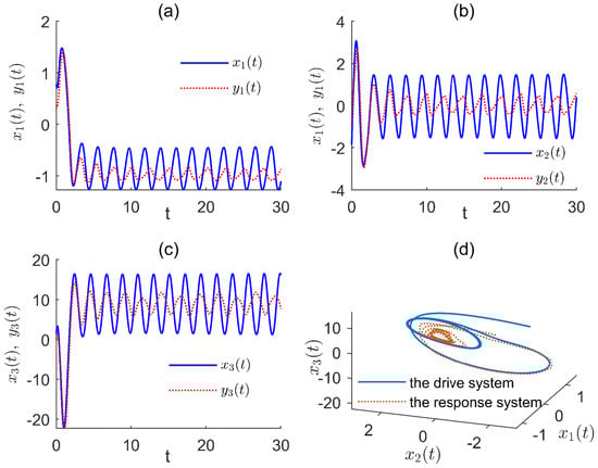
Figure 1. (a) The drive system state $x_1\left(t\right)-t$ space and the response system state $y_1\left(t\right)-t$ space. (b) The drive system state $x_2\left(t\right)-t$ space and the response system state $y_2\left(t\right)-t$ space. (c) The drive system state $x_3\left(t\right)-t$ space and the response system state $y_3\left(t\right)-t$ space. (d) The phase diagram of the drive system and the uncontrolled response system.

Let the nonsymmetric dead zone input nonlinearity be

$$u\left(\alpha \left(t\right)\right)=m\alpha \left(t\right)+\lambda \left(\alpha \left(t\right)\right)=\left\{\begin{array}{cc}m\alpha \left(t\right)-m{\mu }_r,\hfill & \alpha \left(t\right)\ge {\mu }_r,\hfill \\ 0,\hfill & -{\mu }_l<\alpha \left(t\right)<{\mu }_r,\hfill \\ m\alpha \left(t\right)+m{\mu }_l,\hfill & \alpha \left(t\right)\le -{\mu }_l,\hfill \end{array}\right.$$

(74)

where $m=0.8$, ${\mu }_r=14$ and ${\mu }_l=14$. Based on the following rules

• The requested conditions in designing process of controller and for stability of system controlled.
• In order to make comparison, choosing the similar parameters values based on the existed literatures, such as Refs. [13,19,21].

We give the controller and related parameters as follows.

Using the Szász–Mirakyan operator to approximate $H_i\left(Y\left(t\right)\right)$, we have

$$H_i\left(Y\left(t\right)\right)={\theta }_i^T\varphi +{\epsilon }_i\left(t\right),i=1,2,3,$$

(75)

where

$$\left\{\begin{array}{c}{\theta }_i={[H_i\left(0\right)\mu H_i\left({\displaystyle \frac{1}{\mu }}\right){\displaystyle \frac{{\mu }^2}{2!}}{H}_i\left({\displaystyle \frac{2}{\mu }}\right){\displaystyle \frac{{\mu }^3}{3!}}{H}_i\left({\displaystyle \frac{3}{\mu }}\right)...{\displaystyle \frac{{\mu }^N}{N!}}{H}_i\left({\displaystyle \frac{N}{\mu }}\right)]}^T\in R^{N+1},i=1,2,3\hfill \\ \varphi ={[e^{-t}t{e}^{-t}{t}^2{e}^{-t}...t^N{e}^{-t}]}^T\in R^{N+1},\hfill \end{array}\right.$$

and let $N=4$. The command filters are presented as follows

$$\left\{\begin{array}{c}{}_0{}^{C}D_t^{q\left(t\right)}{\psi }_{11}\left(t\right)=w{\psi }_{12}\left(t\right),\hfill \\ {}_0{}^{C}D_t^{q\left(t\right)}{\psi }_{12}\left(t\right)=-2w\vartheta {\psi }_{12}\left(t\right)-w_1({\psi }_{11}\left(t\right)-{\alpha }_1\left(t\right)),\hfill \end{array}\right.$$

and

$$\left\{\begin{array}{c}{}_0{}^{C}D_t^{q\left(t\right)}{\psi }_{21}\left(t\right)=w{\psi }_{22}\left(t\right),\hfill \\ {}_0{}^{C}D_t^{q\left(t\right)}{\psi }_{22}\left(t\right)=-2w\vartheta {\psi }_{22}\left(t\right)-w_2({\psi }_{21}\left(t\right)-{\alpha }_2\left(t\right)),\hfill \end{array}\right.$$

where $x_{2,c}\left(t\right)={\psi }_{11}\left(t\right)$, $x_{3,c}\left(t\right)={\psi }_{21}\left(t\right)$, ${\psi }_{11}\left(0\right)={\alpha }_1\left(0\right)$, ${\psi }_{21}\left(0\right)={\alpha }_2\left(0\right)$, ${\psi }_{12}\left(0\right)=0$, ${\psi }_{22}\left(0\right)=0$ $w=4$, and $\vartheta =0.32$.

The error compensation signals ${\varsigma }_i$ are constructed as

$$\left\{\begin{array}{c}{}_0{}^{C}D_t^{q\left(t\right)}{\varsigma }_1\left(t\right)=-l_1{\varsigma }_1\left(t\right)+{\varsigma }_2\left(t\right)+(x_{2,c}\left(t\right)-{\alpha }_1\left(t\right)),\hfill \\ {}_0{}^{C}D_t^{q\left(t\right)}{\varsigma }_2\left(t\right)=-l_2{\varsigma }_2\left(t\right)-{\varsigma }_1\left(t\right)+{\varsigma }_3\left(t\right)+(x_{3,c}\left(t\right)-{\alpha }_2\left(t\right)),\hfill \\ {}_0{}^{C}D_t^{q\left(t\right)}{\varsigma }_3\left(t\right)=-l_3{\varsigma }_3\left(t\right)-{\varsigma }_2\left(t\right),\hfill \end{array}\right.$$

(76)

where $l_1=2$, $l_2=1.7$ and $l_3=3.7$.

The adaptive laws are given as

$$\left\{\begin{array}{c}{}_0{}^{C}D_t^{q\left(t\right)}{\widehat{\theta }}_1\left(t\right)={\eta }_{11}{\upsilon }_1\left(t\right)\varphi -{\eta }_{11}{\varrho }_1{\widehat{\theta }}_1,\hfill \\ {}_0{}^{C}D_t^{q\left(t\right)}{\widehat{\theta }}_2\left(t\right)={\eta }_{21}{\upsilon }_2\left(t\right)\varphi -{\eta }_{21}{\varrho }_2{\widehat{\theta }}_2,\hfill \\ {}_0{}^{C}D_t^{q\left(t\right)}{\widehat{\theta }}_3\left(t\right)={\eta }_{31}{\upsilon }_3\left(t\right)\varphi -{\eta }_{31}{\varrho }_3{\widehat{\theta }}_3,\hfill \end{array}\right.$$

(77)

in which ${\eta }_{21}=3$, ${\eta }_{31}=3$ and ${\varrho }_2=2$, ${\varrho }_3=2$.

The following is variable fractional order disturbance observers designed

$$\left\{\begin{array}{c}{\widehat{\varpi }}_2\left(t\right)={\chi }_2+c_2{z}_2\left(t\right),\hfill \\ {}_0{}^{C}D_t^{q\left(t\right)}{\chi }_2\left(t\right)=-c_2(z_3\left(t\right)+10y_1\left(t\right)-y_2\left(t\right)-10x_1\left(t\right)-x_2\left(t\right)+{\widehat{\theta }}_2^T\varphi +{\widehat{\varpi }}_2\left(t\right));\hfill \\ \widehat{\sigma }\left(t\right)=\widehat{\tau }+c_3{z}_3\left(t\right),\hfill \\ {}_0{}^{C}D_t^{q\left(t\right)}\tau \left(t\right)=-c_3(-{\displaystyle \frac{100}{7}}{z}_2\left(t\right)+{\widehat{\theta }}_3^T\varphi +\widehat{\sigma }\left(t\right)+m\alpha \left(t\right));\hfill \end{array}\right.$$

(78)

here $c_2=2$ and $c_3=3$.

Finally, the virtual controllers ${\alpha }_1$, ${\alpha }_2$ and the actual controller $\alpha \left(t\right)$ are designed in following form

$$\left\{\begin{array}{c}{\alpha }_1\left(t\right)=-l_1{s}_1\left(t\right)-{\displaystyle \frac{10}{7}}(y_1\left(t\right)-{y_1\left(t\right)}^3)+{\displaystyle \frac{10}{7}}(x_1\left(t\right)-{x_1\left(t\right)}^3)-{\widehat{\theta }}_1^T\varphi -{\widehat{\varpi }}_1\left(t\right),\hfill \\ {\alpha }_2\left(t\right)=-l_2{s}_2\left(t\right)-s_1\left(t\right)-10z_1\left(t\right)+z_2\left(t\right)-{\widehat{\theta }}_2^T\varphi -{\widehat{\varpi }}_2\left(t\right)+{}_0{}^{C}D_t^{q\left(t\right)}{x}_{2,c}\left(t\right),\hfill \\ \alpha \left(t\right)={\displaystyle \frac{1}{m}}({\displaystyle \frac{100}{7}}{z}_2\left(t\right)-{\widehat{\theta }}_3^T\varphi -\widehat{\sigma }\left(t\right)+{}_0{}^{C}D_t^{q\left(t\right)}{x}_{3,c}\left(t\right)-l_3{s}_3\left(t\right)-s_2\left(t\right)).\hfill \end{array}\right.$$

(79)

The state trajectories of the drive system (70) and the response system (72) under the designed controller (79) are illustrated in Figure 2, The Figure 3 is devoted to demonstrate the trajectories of the synchronization errors. From Figure 2 and Figure 3, it can be asserted that the synchronization error signals tend to 0 under the proposed controller.

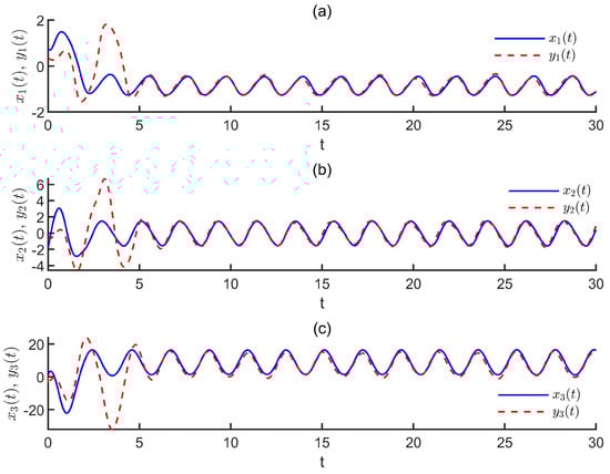
Figure 2. (a–c) The state trajectories of the drive system and the response system with designed controller.

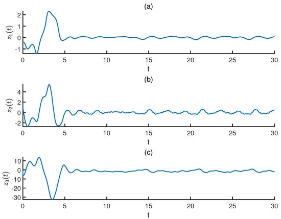
Figure 3. The synchronization errors (a) $z_1\left(t\right)-t$ space, (b) $z_2\left(t\right)-t$ space and (c) $z_3\left(t\right)-t$ space.

The output signals of VO fractional command filters, the error compensation signals, the adaptive laws and the actual controller $\alpha \left(t\right)$ and $u\left(\alpha \right(t\left)\right)$ are depicted by Figure 4, Figure 5, Figure 6 and Figure 7, which indicate that the output signals of command filters, the error compensation signals and the virtual control laws are all bounded. In conclusion, the drive system and the response system are synchronized and the controller design scheme is feasible. The state trajectories of the drive system (70) and the response system (72) under the designed controller (79) without a disturbance observer are presented in Figure 8. From Figure 2 and Figure 8, we can find that better synchronous performance of system under controller with VO fractional disturbance observer.

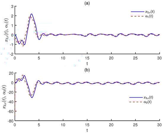
Figure 4. (a,b) The input signals and output signals of the command filters.

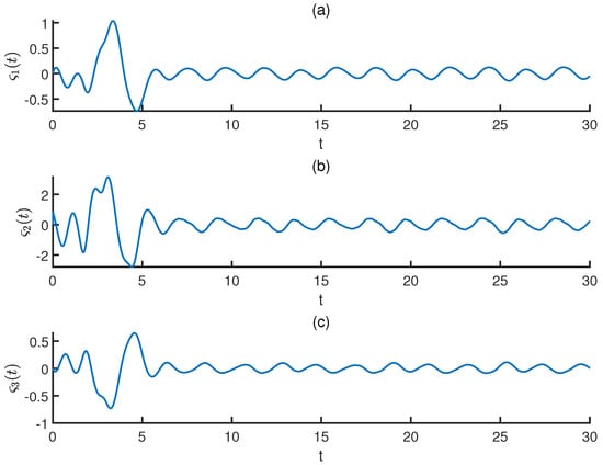
Figure 5. The error compensation signals (a) ${\varsigma }_1\left(t\right)-t$ space, (b) ${\varsigma }_2\left(t\right)-t$ space and (c) ${\varsigma }_3\left(t\right)-t$ space.

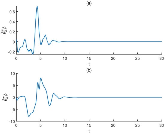
Figure 6. (a,b) The Szász–Mirakyan operators ${\widehat{\theta }}_2^T\varphi -t$ space and ${\widehat{\theta }}_3^T\varphi -t$ space.

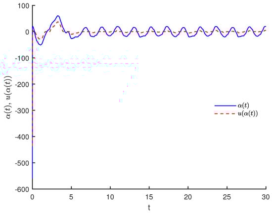
Figure 7. The dead zone input $\alpha \left(t\right)-t$ space and output $u\left(\alpha \right(t\left)\right)-t$ space.

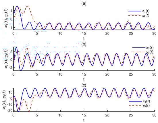
Figure 8. (a–c) The state trajectories of the drive system and the response system without a disturbance observer.

In order to show the control scheme proposed in this paper is better that other, the following comparison with main results obtained in [37] is derived. Let $H_1\left(Y\right)=0,H_2\left(Y\right)=0,H_3\left(t\right)=0,F_1\left(X\right)=0,F_2\left(X\right)=0,G_1\left(Y\right)=0,G_2\left(Y\right)=0,d_1\left(t\right)=0,d_2\left(t\right)=0$ in this paper and $a=0,b={\displaystyle \frac{100}{7}},c=0,d=0$ in [37]. The numerical simulation results on the comparison are expressed by Figure 9 and Figure 10.

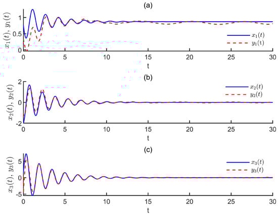
Figure 9. (a–c) The state trajectories of the drive system and the response system with designed controllers in this paper.

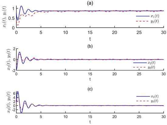
Figure 10. (a–c) The state trajectories of the drive system and the response system with designed controllers in [37].

From the above, it can be found that the synchronization controller with VO fractional disturbance observer and the Szász–Mirakyan operator proposed in this paper can produce the a better performance compared to the controller with adaptive law and fuzzy logic system presented in [37].

5. Conclusions

In this paper, a synchronization control strategy for a class of VO fractional uncertain nonlinear system with external disturbances and dead zone is proposed based on the adaptive BSC technique. The VO fractional command filter derived in this paper can be utilized to suppress “explosion of complexity”in the process of designing controller. The Szász–Mirakyan operator theory is employed to decompose the uncertain nonlinear term into unknown parameters and error functions. A VO fractional disturbance observer can be invoked to overcome the difficulties brought by dead zone and external disturbances. Moreover, the system controlled is stability. Finally, numerical examples indicate the validation of the theoretical results. It must be mentioned that the comparative theoretical results (see Remark 4) and comparative numerical results (see Figure 9 and Figure 10) show the advantage of the proposed control approach in dealing with control problem for VO fractional system with dead zone, disturbances and unknown function.

References

- Podlubny, I. Fractional Differential Equations: An Introduction to Fractional Derivatives, Fractional Differential Equations, to Methods of Their Solution and Some of Their Applications; Elsevier: Amsterdam, The Netherlands, 1998. [Google Scholar]
- Hilfer, R. Applications of Fractional Calculus in Physics; World scientific: Singapore, 2000. [Google Scholar]
- Agarwal, P.; Baleanu, D.; Chen, Y.; Momani, S.; Machado, J.T. Fractional calculus. In Proceedings of the ICFDA: International Workshop on Advanced Theory and Applications of Fractional Calculus, Amman, Jordan, 16–18 July 2018; Springer: Amman, Jordan, 2019. [Google Scholar]
- Samko, S.G.; Ross, B. Integration and differentiation to a variable fractional order. Integral Transform. Spec. Funct. 1993, 1, 277–300. [Google Scholar] [CrossRef]
- Lorenzo, C.F.; Hartley, T.T. Variable order and distributed order fractional operators. Nonlinear Dyn. 2002, 29, 57–98. [Google Scholar] [CrossRef]
- Valério, D.; Da Costa, J.S. Variable-order fractional derivatives and their numerical approximations. Signal Process. 2011, 91, 470–483. [Google Scholar] [CrossRef]
- Patnaik, S.; Hollkamp, J.P.; Semperlotti, F. Applications of variable-order fractional operators: A review. Proc. R. Soc. A Math. Phys. Eng. Sci. 2020, 476, 20190498. [Google Scholar] [CrossRef]
- Almeida, R.; Tavares, D.; Torres, D.F. The Variable-Order Fractional Calculus of Variations; Springer: Berlin/Heidelberg, Germany, 2019. [Google Scholar]
- Jiang, J.; Cao, D.; Chen, H. Sliding mode control for a class of variable-order fractional chaotic systems. J. Frankl. Inst. 2020, 357, 10127–10158. [Google Scholar] [CrossRef]
- Zhou, J.; Wen, C. Adaptive backstepping control. In Adaptive Backstepping Control of Uncertain Systems: Nonsmooth Nonlinearities, Interactions or Time-Variations; Springer: Berlin/Heidelberg, Germany, 2008; pp. 9–31. [Google Scholar]
- Farrell, J.A.; Polycarpou, M.; Sharma, M.; Dong, W. Command filtered backstepping. IEEE Trans. Autom. Control 2009, 54, 1391–1395. [Google Scholar] [CrossRef]
- Ma, J.; Park, J.H.; Xu, S. Command-Filter-Based Finite-Time Adaptive Control for Nonlinear Systems with Quantized Input. IEEE Trans. Autom. Control 2020, 66, 2339–2344. [Google Scholar] [CrossRef]
- Zirkohi, M.M. Robust adaptive backstepping control of uncertain fractional-order nonlinear systems with input time delay. Math. Comput. Simul. 2022, 196, 251–272. [Google Scholar] [CrossRef]
- Izadbakhsh, A.; Khorashadizadeh, S.; Ghandali, S. Robust adaptive impedance control of robot manipulators using Szász–Mirakyan operator as universal approximator. ISA Trans. 2020, 106, 1–11. [Google Scholar] [CrossRef] [PubMed]
- Izadbakhsh, A.; Zamani, I.; Khorashadizadeh, S. Szász–Mirakyan-based adaptive controller design for chaotic synchronization. Int. J. Robust Nonlinear Control 2021, 31, 1689–1703. [Google Scholar] [CrossRef]
- Mei, C.; Guo, D.; Chen, G.; Cai, J.; Li, J. Event-Triggered Adaptive Control for a Class of Nonlinear Systems with Dead-Zone Input. Electronics 2024, 13, 210. [Google Scholar] [CrossRef]
- Dong, G.; Cao, L.; Yao, D.; Li, H.; Lu, R. Adaptive Attitude Control for Multi-MUAV Systems with Output Dead-Zone and Actuator Fault. IEEE/CAA J. Autom. Sin. 2021, 8, 1567–1575. [Google Scholar] [CrossRef]
- Ni, J.; Shi, P. Global Predefined Time and Accuracy Adaptive Neural Network Control for Uncertain Strict-Feedback Systems With Output Constraint and Dead Zone. IEEE Trans. Syst. Man, Cybern. Syst. 2021, 51, 7903–7918. [Google Scholar] [CrossRef]
- Yu, J.; Shi, P.; Dong, W.; Lin, C. Adaptive fuzzy control of nonlinear systems with unknown dead zones based on command filtering. IEEE Trans. Fuzzy Syst. 2016, 26, 46–55. [Google Scholar] [CrossRef]
- Ren, Y.; Zhu, P.; Zhao, Z.; Yang, J.; Zou, T. Adaptive fault-tolerant boundary control for a flexible string with unknown dead zone and actuator fault. IEEE Trans. Cybern. 2021, 52, 7084–7093. [Google Scholar] [CrossRef]
- Bai, Z.; Li, S.; Liu, H.; Zhang, X. Adaptive fuzzy backstepping control of fractional-order chaotic system synchronization using event-triggered mechanism and disturbance observer. Fractal Fract. 2022, 6, 714. [Google Scholar] [CrossRef]
- Xue, G.; Lin, F.; Li, S.; Liu, H. Adaptive fuzzy finite-time backstepping control of fractional-order nonlinear systems with actuator faults via command-filtering and sliding mode technique. Inf. Sci. 2022, 600, 189–208. [Google Scholar] [CrossRef]
- Alassafi, M.O.; Ha, S.; Alsaadi, F.E.; Ahmad, A.M.; Cao, J. Fuzzy synchronization of fractional-order chaotic systems using finite-time command filter. Inf. Sci. 2021, 579, 325–346. [Google Scholar] [CrossRef]
- Ye, H.; Song, Y. Backstepping design embedded with time-varying command filters. IEEE Trans. Circuits Syst. II Express Briefs 2022, 69, 2832–2836. [Google Scholar] [CrossRef]
- Dong, H.; Cao, J.; Liu, H. Observers-based event-triggered adaptive fuzzy backstepping synchronization of uncertain fractional order chaotic systems. Chaos Interdiscip. J. Nonlinear Sci. 2023, 33, 043113. [Google Scholar] [CrossRef] [PubMed]
- Wang, Q.; Cao, J.; Liu, H. Adaptive fuzzy control of nonlinear systems with predefined time and accuracy. IEEE Trans. Fuzzy Syst. 2022, 30, 5152–5165. [Google Scholar] [CrossRef]
- Zhao, J.; Tong, S.; Li, Y. Fuzzy adaptive output feedback control for uncertain nonlinear systems with unknown control gain functions and unmodeled dynamics. Inf. Sci. 2021, 558, 140–156. [Google Scholar] [CrossRef]
- Chen, B.; Lin, C. Finite-Time Stabilization-Based Adaptive Fuzzy Control Design. IEEE Trans. Fuzzy Syst. 2021, 29, 2438–2443. [Google Scholar] [CrossRef]
- Lu, K.; Liu, Z.; Wang, Y.; Chen, C.L.P. Fixed-Time Adaptive Fuzzy Control for Uncertain Nonlinear Systems. IEEE Trans. Fuzzy Syst. 2021, 29, 3769–3781. [Google Scholar] [CrossRef]
- Chen, T.; Yuan, J.; Yang, H. Event-triggered adaptive neural network backstepping sliding mode control of fractional-order multi-agent systems with input delay. J. Vib. Control 2022, 28, 3740–3766. [Google Scholar] [CrossRef]
- Li, Y.; Chen, Y.; Podlubny, I. Mittag–Leffler stability of fractional order nonlinear dynamic systems. Automatica 2009, 45, 1965–1969. [Google Scholar] [CrossRef]
- Ha, S.; Chen, L.; Liu, H.; Zhang, S. Command filtered adaptive fuzzy control of fractional-order nonlinear systems. Eur. J. Control 2022, 63, 48–60. [Google Scholar] [CrossRef]
- Hashtarkhani, B.; Khosrowjerdi, M.J. Adaptive actuator failure compensation for uncertain nonlinear fractional order strict feedback form systems. Trans. Inst. Meas. Control 2019, 41, 1032–1044. [Google Scholar] [CrossRef]
- Zhao, L.; Yang, G.; Luo, K.; He, L. Neuro-adaptive fractional order prescribed performance backstepping control for a class of strict-feedback non-linear systems. IET Control Theory Appl. 2025, 19, e12782. [Google Scholar] [CrossRef]
- Ha, S.; Chen, L.; Liu, H. Command filtered adaptive neural network synchronization control of fractional-order chaotic systems subject to unknown dead zones. J. Frankl. Inst. 2021, 358, 3376–3402. [Google Scholar] [CrossRef]
- Petráš, I. A note on the fractional-order Chua’s system. Chaos, Solitons Fractals 2008, 38, 140–147. [Google Scholar] [CrossRef]
- Ha, S.; Liu, H.; Li, S.; Liu, A. Backstepping-Based Adaptive Fuzzy Synchronization Control for a Class of Fractional-Order Chaotic Systems with Input Saturation. Int. J. Fuzzy Syst. 2019, 21, 1571–1584. [Google Scholar] [CrossRef]
Disclaimer/Publisher’s Note: The statements, opinions and data contained in all publications are solely those of the individual author(s) and contributor(s) and not of MDPI and/or the editor(s). MDPI and/or the editor(s) disclaim responsibility for any injury to people or property resulting from any ideas, methods, instructions or products referred to in the content. |
© 2025 by the authors. Licensee MDPI, Basel, Switzerland. This article is an open access article distributed under the terms and conditions of the Creative Commons Attribution (CC BY) license (https://creativecommons.org/licenses/by/4.0/).