Abstract
Atmospheric turbulence, recognized as a quintessential space–time chaotic system, can be characterized by its fractal properties. The characteristics of the time series of multiple orders of fractal dimensions, together with their relationships with stability parameters, are examined using the data from an observational station in Horqin Sandy Land to explore how the diurnal variation, synoptic process, and stratification conditions can affect the fractal characteristics. The findings reveal that different stratification conditions can disrupt the quasi-three-dimensional state of atmospheric turbulence in different manners within different scales of motion. Two aspects of practical applications of fractal dimensions are explored. Firstly, fractal properties can be employed to refine similarity relationships, thereby offering prospects for revealing more information and expanding the scope of application of similarity theories. Secondly, utilizing different orders of fractal dimensions, a systematic algorithm is developed. This algorithm distinguishes and eliminates non-turbulent motions from observational data, which are shown to exhibit slow-changing features and result in a universal overestimation of turbulent fluxes. This overestimation correlates positively with the boundary frequency between turbulent and non-turbulent motions. The evaluation of these two aspects of applications confirms that fractal properties hold promise for practical studies on atmospheric turbulence.
1. Introduction
Fractals, as a fundamental characteristic of chaotic systems, reflect essential features such as self-similarity and fine structures of specific geometric or dynamic phenomena [1,2,3,4]. Atmospheric turbulence, a quintessential example of a space–time chaotic system, is renowned for its inherent complexity and the challenges it poses for analytical calculations [5,6]. Investigations into the fractal nature of atmospheric turbulence can significantly enhance our comprehension of its governing principles and dynamic properties [4]. Furthermore, such studies can offer valuable insights for addressing practical issues within the atmospheric boundary layer (ABL).
To quantify the properties of fractals, the fractal dimension is introduced to characterize the complexity of certain systems as a ratio of the change in detail to the change in scale [3]. The value of the fractal dimension, which tends to be non-integer, can significantly deviate from the Euclidean or topological dimension. This deviation suggests that the phase-space of the chaotic system is filled differently compared to conventional dynamical systems [4,7,8]. Consequently, the properties of the corresponding system closely align with those of the two integers proximate to the fractal dimension. There exist multiple definitions of fractal dimensions, which, while they may yield identical values for certain systems, fundamentally differ in essence and typically vary in value [9,10,11]. In fact, the diversity in the definitions of fractal dimensions implies the inadequacy of a single index in capturing the dynamics and characteristics of a complex system [12,13,14]. It has been demonstrated that the majority of existing definitions can be generalized into infinite orders of multifractal dimensions, thereby enabling the properties of a fractal to be described by different orders of dimensions [15,16].
The multifractal characteristics are fundamentally pervasive, spanning from natural phenomena [17,18,19] to creature physiology [20,21,22]. The study of fractals also extends its applicability to practical domains within social and economic sciences [23,24,25]. Within the realm of fluid turbulence, the exploration of properties associated with fractal characteristics has remained a consistent area of focus over the past several decades. For example, Meneveau and Sreenivasan [26] discussed the experiment-based intermittency of the rate of turbulent energy dissipation and concluded that the distribution of the dissipation field has a multifractal nature which corresponds to f(α) models put forward by Halsey et al. [27]. Benzi et al. [28] analyzed the probability distribution functions of the velocity gradients in fully developed turbulence and endowed the turbulence with multifractality based on the relationships between the exponentials of structure functions and turbulence statistics such as Reynolds number. Lovejoy and Schertzer [29] put forward and recommended methods in quantifying the fractal structures concerning the turbulence in the atmosphere and ocean. Alberti et al. [15] combined the concept of empirical mode decomposition and generalized fractal dimension together to characterize the multifractal features of typical chaotic dynamical systems, and this methodology was further used in the practices of other chaotic systems such as coupled ocean–atmosphere and solar wind magnetic field [30,31]. Carbone et al. [32] investigated the local dimension and the inverse persistence of the atmospheric turbulence in a stable boundary layer from CASES-99, and they verified that these two metrics could serve as indicators of characteristics of dynamical systems. There are also numerous contemporary studies integrating fractal properties into practical applications that are correlated with human lives [33,34,35]. In the studies of fractal properties of atmospheric turbulence, researchers are inclined to integrate established methods together with traditional turbulence theories, such as the K41 theory [36]. In this situation, the maturely developed Monin–Obukhov similarity theory (MOST), which describes the laws of turbulence and the boundary layer through the combined dimensionless variables [37,38], can also be prospective with the ingredients of multifractal dimensions, as the latter themselves are already dimensionless numbers. Furthermore, as the past research has suggested the utility of fractal dimension in the characteristics of atmospheric turbulence, specific practices based on the multifractal nature of turbulence are also to be urgently verified.
In this study, the characteristics of fractal dimensions of atmospheric turbulence are investigated, using observational data collected from Horqin Sandy Land, an area with a near-ideal underlying surface. The time series of fractal dimensions of different orders are examined for diurnal patterns and extrema, from which the physical mechanisms by which the stratification states and synoptic conditions influence fractal properties is discussed. The similarity relationship based on fractal dimensions will be explored and used to refine the relationships in Monin–Obukhov similarity theory. Drawing upon these characteristics, unearthed from time series and similarity relationships, a systematic algorithm is proposed. This algorithm, predicated on the Hilbert–Huang transform method, distinguishes the influences from motions of varying scales on the fractal dimension. It can be employed to discern the boundary between turbulent and non-turbulent motions from observational data. Furthermore, a quantitative investigation is conducted into the efficacy of this method in reconstructing time series of atmospheric turbulence and the turbulent flux, which justifies the utility of exploring fractal characteristics and can provide preference on the selection of parameterization schemes pertaining to the processes of atmospheric turbulence and the ABL.
2. Data and Methods
2.1. Observational Site and Instruments
The observational station was selected at the Horqin Sandy Land (42°56′ N, 120°42′ E), which is located in the Naiman County of Inner Mongolia, China. There is a typical semi-arid continental monsoon climate, and the vegetation around the Horqin station mainly contains low and open shrubs [39,40,41], which guarantees a nearly ideal homogeneous and flat underlying surface for observation. Detailed information about other observations of the Horqin station can be found in Li and Zhang [39]. The observational data span is 1 month for each of two cases, which are July and December in 2022.
The data from a 20 m meteorological observational tower (Tower 1) and another 2.2 m independent observational tower (Tower 2) are used, which are located about 10 km to the north of downtown Naiman, with an altitude of 363 m. For Tower 1, there are eddy covariance (EC) systems at 4, 8, and 16 m, which contain three-axis sonic anemometers (CSAT3, Campbell Scientific Co., Logan, UT, USA), for determining the 3-dimensional wind speeds and virtual temperature fluctuations, and an open path gas analyzer (LI-7500, LI-COR Biosciences, Inc., Lincoln, NE, USA), for determining the fluctuations in CO2 and H2O density. For Tower 2, the same set of a sonic anemometer and open path gas analyzer were installed at the height of 2.2 m. The sensors of all the instruments were oriented west (270°), and their sampling frequency was 10 Hz. Figure 1 illustrates the layout of these instruments.
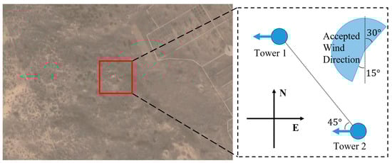
Figure 1.
Location and layout of the instruments (left panel from Google Maps); blue circles denote 2 observation towers, arrows mark orientation of sensors, and sector shows direction range of accepted data.
2.2. Data Pre-Processing and Selection
The raw turbulence observational data were pre-processed using the EddyPro software (Advanced 7.0.9, LI-COR Biosciences, Inc., USA), including error flags, despiking [42], double coordinate rotation, and detrending. The averaging time scale of the pre-processing was 30 min. Based on the Reynolds decomposition, several kinds of characteristic scales and parameters concerning conditions of turbulence and the ABL can be defined by the following:
where
denotes the fluctuation term,
is the friction velocity,
is the characteristic scale of temperature,
is the Obukhov length, and
is the stability parameter that reflects the stratification state by a division of height
and Obukhov length. To remove inaccuracies caused by the field observations and reveal the connections of the two towers, data meeting one of the following criteria were rejected:
- (1)
- either the angle between the sonic anemometer sensing probe and wind direction or the angle between the connector of the two towers and wind direction was larger than ±120 (accepted wind direction range is shown in Figure 1);
- (2)
- the mean wind speeds were smaller than 0.5 m/s or larger than 5 m/s;
- (3)
- the friction velocity was smaller than 0.05 m/s;
- (4)
- the absolute value of sensible heat flux was smaller than 5 .
2.3. Method of Hilbert–Huang Transform
The method of Hilbert–Huang transform, recognized for its proficiency in managing non-linear and non-stationary signals with multiple components [43,44,45], proves particularly effective when applied to atmospheric turbulence data. This study leverages this method to distinguish between turbulent and non-turbulent components within the observational data. The fundamental steps of the Hilbert–Huang transform are as follows:
- (1)
- Conducting Empirical Mode Decomposition (EMD):
EMD is an algorithm used to decompose a real signal
into a sum of intrinsic mode functions
and a residual function
. For each intrinsic mode function (IMF), it satisfies two criteria: (a) the difference between the number of local extrema and the number of zero-crossings must be zero or one; (b) the running mean value of the envelope defined by the local maxima and the envelope defined by the local minima is zero. IMFs can be acquired by repeatedly finding and subtracting the “local means” from the signal. For the time series of a single variable, this can be directly achieved by identifying the envelopes of local maxima and minima (which can be called univariate EMD or traditional EMD), yet for time series of multiple variables or when it is necessary to take combined variables into consideration, some subtle steps in defining and calculating local means are needed (which are referred to as multivariate EMD [46,47,48]).
- (2)
- Performing the Hilbert transform for each IMF according to the definition:
Small numbers of
correspond to motions of high frequencies and small scales, and large numbers of
(up to 14–16, empirically) are accordingly the low-frequency and large-scale motions. It is revealed that non-turbulent motions often occur at IMFs of large numbers of
and residual signals [49,50], and the searching of the boundary between turbulent and non-turbulent motions is crucial and to be investigated.
- (3)
- Calculating the Hilbert marginal spectrum:
With the time series of
and
, the Hilbert spectrum,
, can be defined as a frequency–time distribution of the amplitude, and the Hilbert marginal spectrum
can be defined as an integral of
within the data sample of size
:
From the time series of
and
for each IMF, the joint probability density functions (PDF)
can be calculated. According to joint PDF, the arbitrary-order Hilbert marginal spectrum can be defined in an amplitude–frequency space by a marginal integration of the joint PDF as
where
and
are the instantaneous frequency and instantaneous amplitude at time
, respectively.
Generally, the method of Hilbert–Huang transform can be seen as an adaptive method, which can be used in the analysis of non-linear and non-stationary signals. Compared to Fourier transform and the traditional second-order structure function, the Hilbert spectra analysis has been proved to be more capable of revealing larger-scale structures’ intermittency of turbulence [51]. However, there are some problems that exist in the applications of Hilbert–Huang transform, such as the arbitrariness, the end effect, and the mode mixing problems of EMD, and therefore some improvements [52,53,54,55] can be applied to this method to make it more effective and reliable.
2.4. Calculation of Fractal Dimensions
Atmospheric turbulence is worth exploring through multifractal properties for its time–space chaotic nature. The arbitrary order of a fractal dimension has been proved able to be directly calculated from the time series of observational data [15,16], which follows:
where
denotes the qth order of fractal dimension,
is the size of the hypercube in phase-space (referring to the 3D Euclidean space generated by u-, v-, and w-wind speed in this study), and
is the probability of the ith hypercube that is being visited by the trajectory. The different orders of
describe the multifractality of a certain dynamical system as they can be attributed to different scale-independent processes. For the 3-dimension motions of atmospheric turbulence, the orders below should be specially analyzed:
with
being called capacity dimension, information dimension, and correlation dimension, respectively. The data samples of calculating dimensions are also set to be 30 min.
is the number of hypercubes in the phase-space that contain trajectory points,
is the Shannon entropy, and
is the correlation integral.
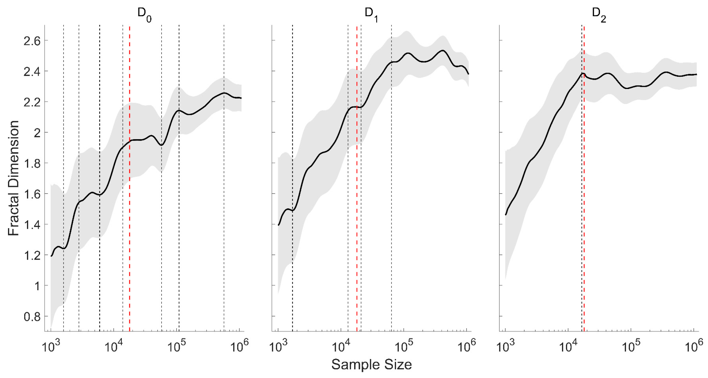
By definition, fractal dimensions require an infinitesimal value of hypercube selected in phase-space and an infinite data length to acquire the true value of probabilities, and there is
. Figure 2 visualizes the influence of sample size on the calculated fractal dimensions, showing that with the increase in sample size,
and
increase in a stepwise way, and
increases and converges near a sample size of
, which implies that the statistical methods of estimating
and
perform better than the box-counting algorithm of
. As the pursuit of accuracy comes at a significant computational cost, and the expansion of data sample may include the motions of a larger scale than turbulence, the data samples are selected as 30 min intervals in this study, following the standardized practical applications (such as estimating turbulent fluxes). Additionally, the L’Hôpital’s rule can be conducted with respect to the variable
to improve computational accuracy and efficiency.
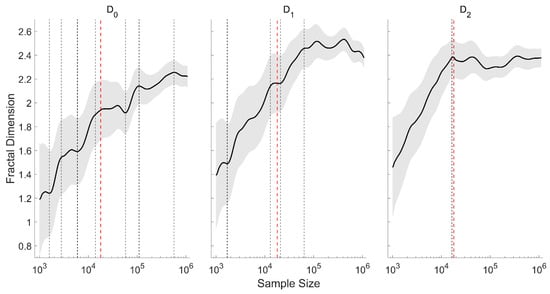
Figure 2.
The relationship among the sample size and the fractal dimensions of different orders for 20 random cases. The black dashed lines mark the stages of the increased dimensions, the red dashed line denotes the sample size chosen in this study, and the gray area denotes the standard deviation.
2.5. Fractal Dimensions Refining Similarity Relationships
For the similarity relationships concerning dynamics properties of atmospheric turbulence, the empirical relationships are proved to be satisfying “1/3” exponential relationships:
where
is the variable that is of concern,
is the corresponding characteristic scale defined in Equations (1)–(4),
is the stability parameter, and
and
are the fitted coefficients. It turns out that the relationship of
with the stability parameter is similar to that of
, and by multiplying
by a factor
, the similarity relationship can be refined with their outliers offset, and the new parameter still satisfies a “1/3” exponential relationship:
where
, and
are the new fitted coefficients. Notice that the fractal dimensions are calculated from the wind speeds of three directions; the normalized standard deviation of potential temperature can NOT be refined in this way.
Apart from the normalized standard deviation, the normalized cross-correlation coefficients are also worthy of exploring similarity relationships due to their strong link with turbulent fluxes:
where
are the two variables that are of concern,
denotes their covariance, and
are the standard deviations of the two variables. For the standard deviations that satisfy the similarity relationship in Equation (14), the cross-correlation coefficients are suggested to satisfy the relationships as follows [56,57,58]:
where the coefficients A and B are all acquired from the fitted curves of normalized standard deviation. As the empirical relationships concerning the normalized cross-correlation coefficients are highly dependent on the ones concerning the normalized standard deviation, the fractal dimension-refined relationships can accordingly be written as follows:
based on the inverse 2 order of u- and w-wind’s standard deviations in the definition of
, and the inverse 1 order of w-wind’s standard deviation of
(as the relationship based on potential temperature is not refined by fractal dimensions).
The effectiveness of refining similarity relationships can be justified in two ways: more information revealed by the new similarity relationship; higher goodness-of-fit indexes, which can be defined by the following:
where RMSE is the root mean square error reflecting the degree of dispersion from data points to fitted curves,
is the total number of data points,
is the predicted value from the fitted curve, and
is the real value. The RMSE can be of reference on the reliability of the similarity relationship.
2.6. Fractal Dimensions Reconstructing Turbulence Data
The EMD process in Section 2.3 decomposes a turbulence signal into several IMFs, and for idealized turbulence, the fractal dimension is constant regardless of how many IMFs are revolved. However, it turns out that for the observed data, the fractal dimensions of the combinations of different IMFs tend to be different. This means the self-similarity is lost for a certain scale, at which the properties and types of motion are also deviated from the other scales. By superimposing the IMFs of the signal from high frequencies to low frequencies (namely from a small to large scale), the change in dimension can reveal the compositions and the properties of the signal. Based on sufficient data samples, the qth order of fractal dimensions at frequency
can be defined as the average fractal dimension calculated from the sum of IMFs from 1 to k:
where the frequency of the kth IMF is around
. From the changing pattern, one can summarize a systematic algorithm to distinguish the turbulent and non-turbulent motions from the time series, and further reconstruct the turbulent fluxes in practical use.
The pre-processing of data collected from sonic anemometers can effectively eliminate the outliers and errors caused by the instruments. However, the non-turbulent motions can not be distinguished. As the atmospheric turbulence and the non-turbulent motions are different in scale, it is reasonable to practically suppose a boundary frequency,
, between turbulent and non-turbulent motion, and the time series can then be written as follows:
where
contains the signal with frequencies higher than
, and
contains the signal with frequencies lower than
. To extract two parts of signals from the original data, the number of IMFs with a frequency closest to
should be located as
, and these two kinds of signals can be calculated as follows:
In this way, the turbulence data are reconstructed as
. In practice, the original data usually go through Reynolds decomposition and are divided into
and
, and after reconstruction,
can act as a substitution of pure turbulence data without the influence of non-turbulent motions. And the derivatives of turbulence data, such as the sensible heat flux
, momentum flux
, CO2 flux
, and latent heat flux
, can also be calculated using the reconstructed data:
where
is the potential temperature;
and
are the air density and specific heat capacity at constant pressure;
is the concentration of carbon dioxide;
is the latent heat; and
is the concentration of water vapor, respectively.
In order to elucidate the systematic algorithm associated with the Hilbert–Huang transform method and the reconstruction of turbulence data through the analysis of fractal dimensions, a flow chart in Figure 3 is given as a visual aid to facilitate a deeper understanding of the intricate processes involved.
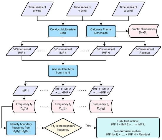
Figure 3.
Flow chart of conducting Hilbert–Huang transform and reconstructing turbulence data with the help of fractal dimensions.
3. Characteristics of Fractal Dimensions
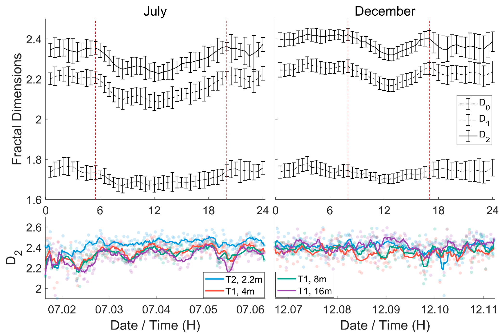
3.1. Time Series of Fractal Dimensions
Figure 4 presents a time series of fractal dimensions in July and December 2022, observed at various towers and heights, and the averaged diurnal patterns. The values of dimensions are observed to increase with the fractal order, and the comparison among the three orders of dimensions reveals that
, which reflects the topological properties, remains stable for most of the time in July but exhibits variability in December. From Figure 2, it can be judged that the although
is not converged for the current sample size, it reaches a steady “step” where the motions of typical scales of turbulence are all included. In this condition,
fluctuates around 1.7, which is lower than the theoretical value of 7/3 for fully developed turbulence in the isotropic system [59,60]. This implies that for atmospheric turbulence, the underlying surface and the stratification conditions may profoundly affect the motions, and the observed flow experiences diverse processes that disrupt its self-similarity. Consequently, the resulting behavior deviates from the ideal and isotropic pictures, revealing distinct patterns. On the other hand,
and
reflecting information and correlation properties reach the convergence and display clear and similar diurnal patterns with minima at around 12:00 every day, with average values of around 2.2 and 2.4, separately. Furthermore, with the height increasing, the values of
and
decrease, with an increased variation, showing a more distinguished pattern. This means that
can only reflect the overall pattern of atmospheric turbulence and is incapable of distinguishing the properties among different stratifications. In contrast, the 1st and 2nd orders of the fractal dimension reflect similar information concerning stratification states from their diurnal patterns, implying the finiteness of the fractal nature of atmospheric turbulence. The difference between heights and the diurnal pattern is comparatively clear in July and is less distinguishable in December. However, in the latter condition, the time-localized variation suggests that the fractal dimension can be more susceptible to synoptic processes in December, as evidenced by the local minima in the nighttime around 10 December.

Figure 4.
The diurnal pattern and time series of fractal dimensions in July and December 2022, the left 2 panels for July, and the right ones for December. The error bars in the top 2 panels denote the 95% confidence intervals, and the erect dashed lines denote the times of sunrise and sunset. The blue, red, green, and purple points/lines in the bottom 2 panels denote the data from Tower 2 (with the height of 2.2 m) and Tower 1 with the height of 4 m, 8 m, and 16 m, respectively.
The diurnal pattern and the variations among different heights suggest a correlation between the dominant wind speed, the vertical wind speed, and the fractal dimensions
and
, as the dominant wind speed is modulated by surface friction, while the vertical wind speed is governed by daily thermal circulations. For measurements taken at higher positions and during the daytime, both types of wind speed tend to be higher. Given that the background values of vertical and cross wind are relatively low, any wind component exceeding this scale can lead to a decrease in the fractal dimension. This is due to the disruption of self-similarity between large and small scales in the motion and suggests a scale-dependent nature of the fractal dimensions.
The observed differences between July and December can be ascribed to the seasonal variations in stratification conditions. In December, the turbulent kinetic energy (TKE) input is diminished, with a prevailing condition of a gentle breeze, thereby blurring the differences among heights and the diurnal pattern. However, under such conditions, the fractal dimension exhibits heightened sensitivity to synoptic processes and motions other than turbulent motion, such as sub-mesoscale motions. Consequently, the data from July can be more effective in revealing the quantitative characteristics of fractal dimensions.
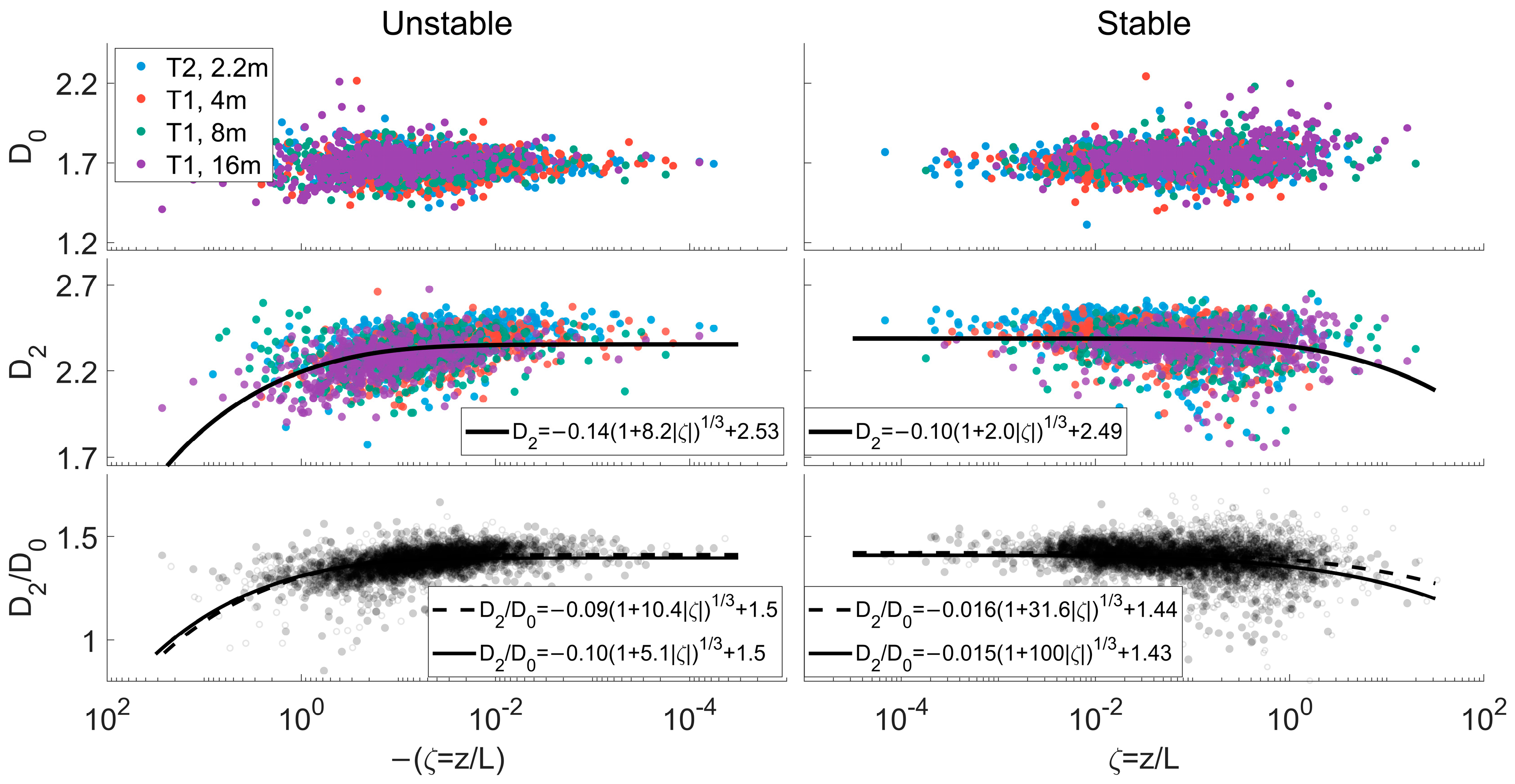
3.2. Similarity Relationship of Fractal Dimensions
As previously illustrated, the dimensionless attribute of fractal dimensions renders them suitable for testing in similarity relationships. Figure 5 portrays the relationship concerning fractal dimensions and the stability parameter, and the result of
is omitted for its similar pattern to
. The fractal dimensions remain stable for a small absolute value of
, and as
increases, the discreteness of dimensions also enlarges. For
, given that the time series exhibits a stable pattern, it scarcely reflects any laws associated with stratification conditions. As a geometric measure of the fractal dimension, the inability of its convergence makes it only reflect the minority of self-similarity, such as the two-dimensional eddies of the turbulence. In contrast,
and
describe the self-similarity from information and correlation aspects, which proves a better performance and displays similar and steadily descending patterns as the absolute value of
increases. Moreover, the distribution of different-colored data points suggests that the different ranges of fractal dimension calculated from various heights can complement each other in the comprehensive picture of the similarity relationship. From the fractal dimension
, it is discerned that the decrease in fractal dimension with the increase in the absolute value of
exhibits a slightly different pattern between unstable and stable stratification conditions. However, both can be fitted into 1/3 exponential relationships, which elucidates that in neutral conditions, the dimension tends to converge around 2.4.
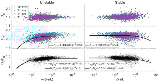
Figure 5.
The similarity relationship based on fractal dimensions. The left panels for unstable stratifications and the right for stable ones; the top 4 panels for the relationship between
,
, and the stability parameter in July 2022, with the same colors as Figure 4. The 3rd row for the ratio
with the solid lines and points for July, and the dashed lines and hollow points for December.
The observed descending pattern suggests that under near-neutral conditions, the atmospheric turbulence exhibits near-isotropic structures. In this situation, the weakly unstable/stable stratification plays a minor role in the development of turbulence. Consequently, turbulent motion exhibits increased self-similarity, reflected in a higher value of the fractal dimension. However, the patterns between strongly stable and unstable conditions, while similar, depict different pictures. When the stability parameter is less than 0 with a large absolute value, the influence of buoyancy becomes dominant, and the atmospheric turbulence obtains energy from the large-scale motions such as local circulation. The fractal dimension thus decreases to reflect more properties of these quasi-two-dimensional motions. On the contrary, when the stratification is strongly stable, the motion of atmosphere is strongly constrained by the dynamics of the inversion layer, and the horizontal motions represented by sub-mesoscale motions would take charge, making the fractal dimension also decrease. In these two limiting cases, despite the fractal property suggesting non-turbulent motions of lower dimension and higher anisotropy, it has been demonstrated that isotropic motions within the inertial subrange can be restored and potentially separated using generalized fractal dimensions and the Hilbert spectra [49,61]. This theoretical foundation enables the reconstruction of turbulence data based on the fractal properties.
Although the distribution of
and
at high absolute numbers of stability parameters is relatively scattered, their ratio displays a concentrated relationship with a 1/3 exponential pattern, as the third row in Figure 5 shows. This is because the ratio of
and
serves as a measure of the multifractality at a certain sample size. As discussed before, in a condition where
is only able to reflect minor fractal properties and
reaches convergence and describes the overall self-similarity, their ratio essentially quantifies to what extent the multifractal nature brings the divergence to the different measures of fractal dimensions. This multifractality is dependent not on only the data sample (mostly on the convergence of
) but also on the stability parameter
, since the development of turbulence is profoundly influenced by the stratification conditions. Therefore, the term
can be effective in reflecting both the self-similarity and the degree of multifractals. The difference in large numbers of stability parameters also makes it feasible to reflect the thermodynamic conditions among different seasons, thereby ensuring its potential for practical use in similarity relationships.
4. Similarity Relationship Refined by Fractal Dimensions
4.1. Refined Relationships of Dynamic Properties
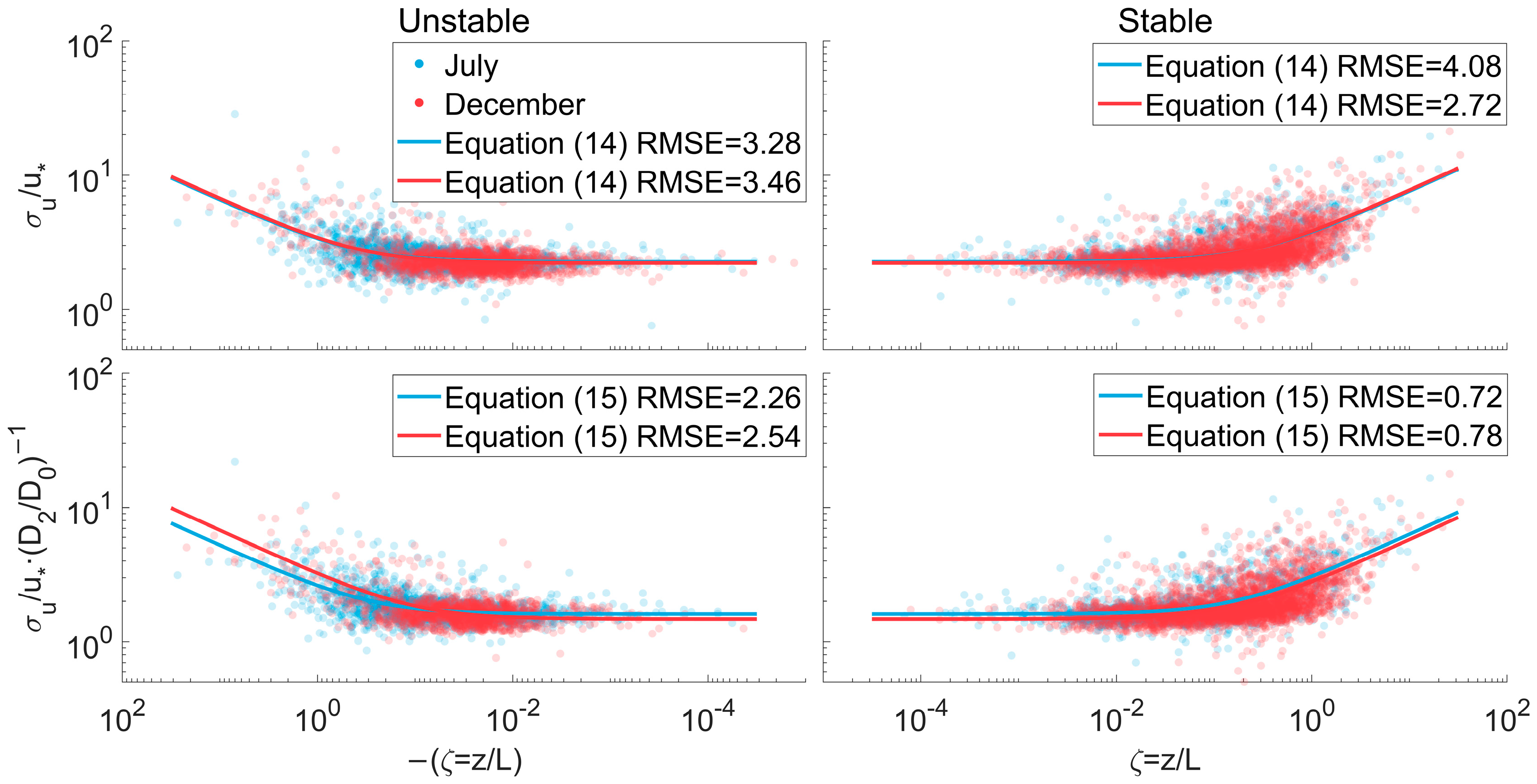
As is analyzed in Section 3.2, the ratio of different orders of fractal dimensions demonstrates a consistent pattern in response to changes in the stability parameter. Consequently, investigations into the similarity relationships, refined by fractal dimensions, could be employed to examine how fractal properties can augment traditional similarity relationships, thereby expanding their feasibility and scope of application. Figure 6 compares the result of free-coefficient fitting of Equations (14) and (15) for the similarity relationships of the normalized standard deviation of u-wind and its fractal dimension-refined variable. It can be judged that the introduction of the term
does not affect the data dispersion and the shape of fitted curves to a large extent. However, the advantage of the fractal dimension term in similarity relationships can be justified through the goodness-of-fit, as the refined relationships universally show smaller RMSE, namely a decrease in the degree of dispersion. This means that in practical applications, the fractal dimension can help retrieve the turbulence statistics in a more precise way, and some outliers which might be eliminated in traditional relationships can also be included in consideration.
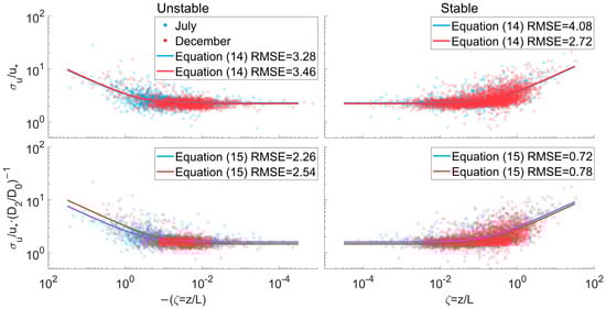
Figure 6.
The comparison of similarity relationships of normalized u-wind standard deviation and the fractal dimension-refined relationships in July and December 2022. The points denote the original dimension data and are semi-transparent processed, and the lines are the fitted curves. The blue ones are for the results in July, and red ones for the results in December.
To further explore the effectiveness of the fractal dimension term
, the comparison of the left two panels in Figure 6 implies that in unstable stratifications where the development of turbulence can be diverse, the difference in thermal conditions can be identified, especially for large absolute values of stability parameters. In July, the stronger radiation promotes the development of turbulence in a more isotropic way, namely
overweighs
to a larger extent, and the refined variable with the term
would decrease. In this condition, the refined similarity relationship in July shows a milder pattern compared with that in December. For the normalized standard deviation of w-wind, the similarity relationships are also refined using the factor
and are fitted into the same empirical relationships as Equations (14) and (15), and the results are omitted to avoid redundancy.
There may be a potential misunderstanding that the observed decrease should be solely attributed to the reduction in overall values as a result of the fact that
. However, this is not the case. When the normalized standard deviation of u-wind is adjusted by
(which has been tested not to have a distinguishing effect) rather than
with increased overall values, the goodness-of-fit still shows a better consequence. In fact, the introduction of
accentuates the discrepancy among different stratification conditions, resulting in more differentiated relationships. The goodness-of-fit further confirms that the distinguishing and error-tolerant effect is inherent to
, rather than being a data illusion. Detailed statistics of the goodness-of-fit will be presented in Table 1 at the end of this section. The refining term is not confined to
itself. Its utility is derived from the additional information of multiple orders of self-similarity that other variables fail to encompass. Therefore, the exploration of more combinations of fractal dimensions in the refinement of similarity relationships holds promising prospects.

Table 1.
The goodness-of-fit for different kinds of dimensionless variables in similarity relationships of dynamic properties.
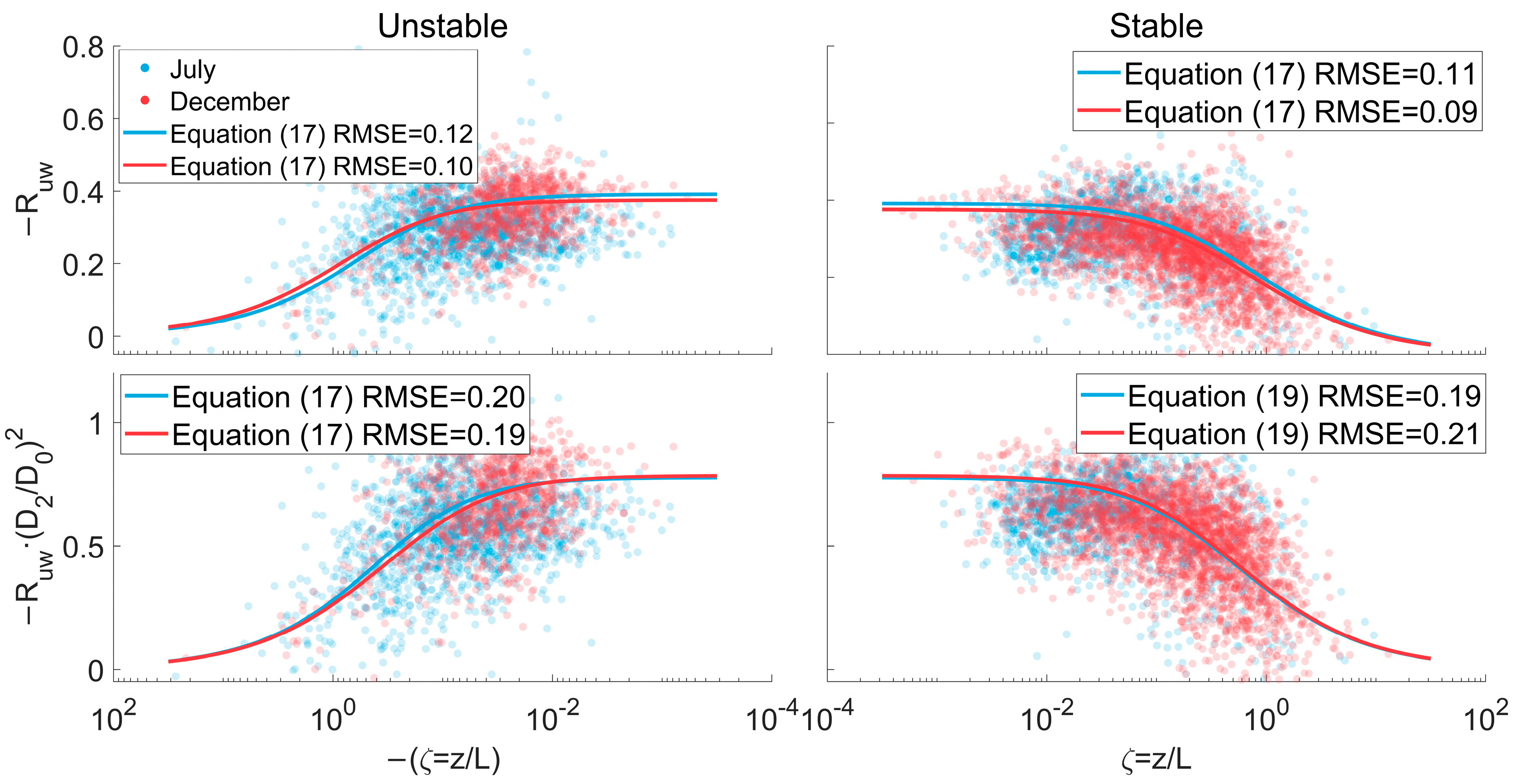
Figure 7 illustrates the similarity relationships of the normalized cross-correlation coefficient of u and w-wind, along with its fractal dimension-refined variable. The fitted curves, based on Equations (17) and (19), are derived using the fitted parameters from the similarity relationships of the normalized standard deviation, as outlined in Equations (14) and (15). No new parameters are introduced. It is revealed that in the similarity relationships of the original normalized cross-correlation coefficient, the differences between July and December are primarily observed in the large (
) and small (
) absolute values of stability parameters, where the data points are sparse and can only reflect minor cases. For the fractal dimension-refined coefficient, the difference at around
of the absolute stability parameter can be distinguishable, which can serve as a new reference for the variations in stratification conditions. Furthermore, the results of the goodness-of-fit suggest that while the factor
amplifies the average absolute values of the coefficient, the reliability remains unaffected and consistent.

Figure 7.
The comparison of similarity relationships of normalized cross-correlation coefficients of u and w-wind (top 2 panels) and the fractal dimension-refined relationships (bottom 2 panels) in July and December 2022. For line and point styles, please refer to Figure 6.
4.2. Refined Relationships of Thermodynamic Properties
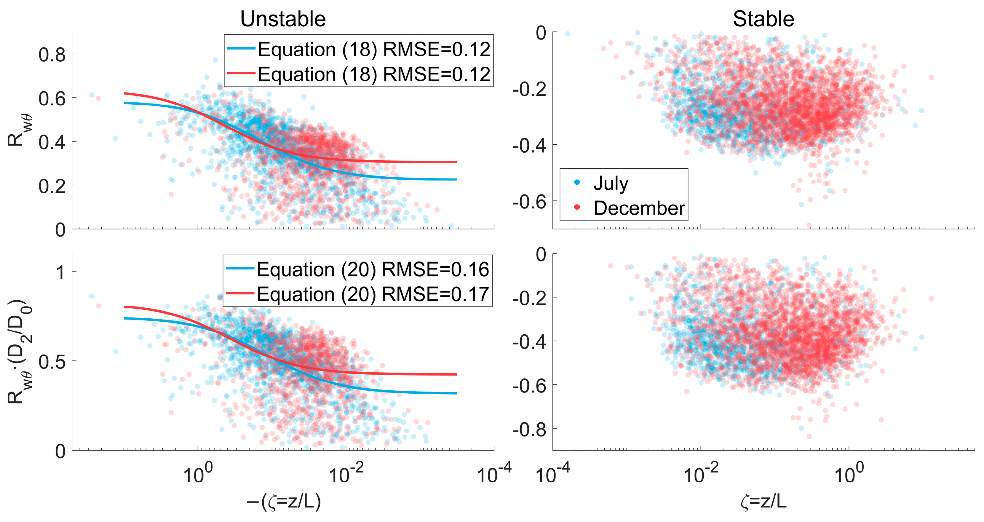
As the fractal dimensions are calculated from wind speed, the normalized deviation of potential temperature will not be adjusted by the fractal dimensions, but the coefficients from the fitted curve will still be useful, as suggested by Equations (18) and (20). In Figure 8, the normalized cross-correlation coefficient of w-wind and potential temperature is refined using the factor
according to the inverse 1 order of the w-wind standard deviation. The data in unstable stratifications are fitted into empirical relationships as outlined in Equations (18) and (20). While the fitting effects are not as robust as those observed for dynamic properties, the refined similarity relationship reveals a larger difference between July and December in the large (
) and small (
) absolute values of stability parameters, and a smaller difference at around
, which is just the opposite to the effect of fractal dimensions to dynamic properties. This can also help retrieve the turbulence statistics concerning the heat flux.
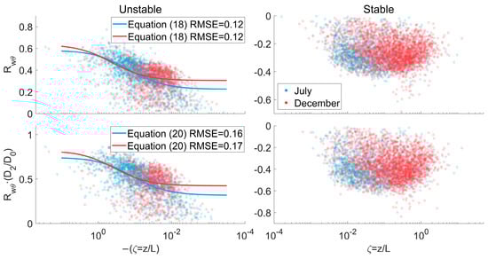
Figure 8.
Comparison of similarity relationships of normalized cross-correlation coefficients of w-wind and potential temperatures (top 2 panels), and the fractal dimension-refined relationships (bottom 2 panels) in July and December 2022. For line and point styles, please refer to Figure 6.
From the analysis conducted above, it is evident that turbulent momentum and sensible heat transport can be significantly improved across a broader range of stratification conditions. Furthermore, this enhancement allows for more precise and distinguishing assessments. As the diurnal patterns of fractal dimensions of different thermal conditions are summarized in Figure 4, similarity relationships can be established for various scenarios (e.g., different seasons and synoptic conditions). The discussions based on Figure 6, Figure 7 and Figure 8 provide a solid foundation for this approach. In practical applications, refined similarity relationships can be empirically derived from historical data, and by incorporating standard meteorological parameters alongside the fractal dimensions, turbulent fluxes can be estimated and predicted. Additionally, considering scalars as additional independent dimensions—specifically, the three wind speed directions in conjunction with the temperature and density of gasses such as CO2 and water vapor—enhances the reliability of refining these similarity relationships. While this approach would increase the computational cost, it would enhance the reliability of the refinement on the corresponding similarity relationships.
5. Reconstruction of Turbulent Fluxes by Fractal Dimensions
As the loss of self-similarity at a certain scale implies the shift in properties of motion, it is postulated that reconstructing turbulence signal from the superimposed IMFs can reveal the boundary between turbulent and non-turbulent motions. In this situation, the turbulent fluxes can be corrected, with non-turbulent motions eliminated. As the data in July contains more fully developed turbulence cases and no fewer non-turbulent motions (e.g., plumes and thermals in daytime and sub-mesoscale motions in nighttime), the statistical and case analysis are conducted for data in July, and the results are also verified for data in December and other sources.
5.1. Fractal Dimensions Influenced by Scale
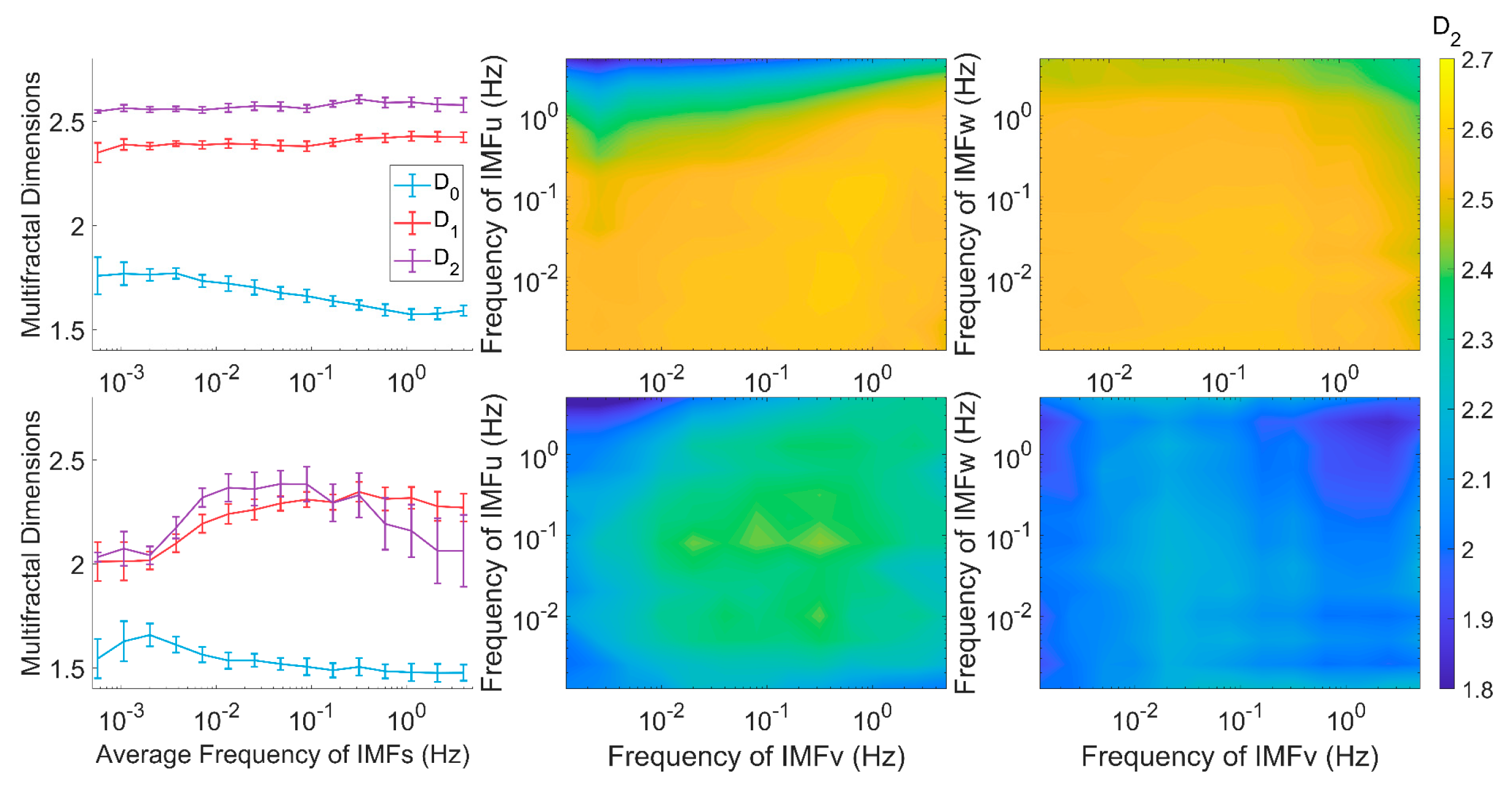
Figure 9 displays the relationship between the fractal dimension and superimposed IMFs in two different ways. For the left two panels, the IMFs are acquired by multivariate EMD, and the frequency is the average of u-, v-, and w-wind within the same number of IMF; for the remaining four panels, the IMFs are acquired by traditional univariate EMD, and the relationships are displayed in pairs of IMFs. It can be judged from the left two panels that the dimensions
steadily increase as the IMFs are superimposed from high to low frequencies, while
decreases with the superimposition. For the top 5% percentiles of
(most of which are from stable boundary layer), it decreases as large-scale motions are superimposed, but the bottom 5% percentiles of
(which represent unstable boundary layer) experience an increase and decrease process with high uncertainty. In stable conditions, as the motions are simple, the system is free to explore the phase space, and the motions of larger scales make little difference, or sometimes promote the self-similarity. On the contrary, the current sample size sometimes makes the system unable to explore the entire phase-space in unstable conditions, and the non-turbulent motions of the larger scale intensify the anisotropy and introduce the abnormal properties of fractal dimensions, especially
.
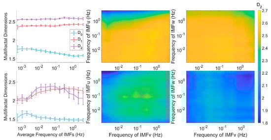
Figure 9.
The relationship between the average fractal dimensions and the frequency of superimposed IMFs in July 2022. The left 2 panels for multivariate EMD, and the remaining 4 panels for univariate EMD; the top 3 panels correspond to stable stratifications and the bottom ones for unstable stratifications. The blue, red, yellow, and purple lines denote
and
, and the error bars for the 95% confidence intervals of each point.
While the results of multivariate EMD reveal the overall pattern of the fractal dimension and superimposed IMFs, the results from univariate EMD provide comparative patterns in pairs of IMFs from the univariate EMD for the top and bottom 5% percentiles of fractal dimensions, which correspond to stable and unstable stratification conditions. It can be seen from the middle two panels that when w-wind is kept unchanged, as the IMFs of u-wind are superimposed from small scale to large scale (from the top to bottom and right to left of the panels), the fractal dimension
increases, and the superposition of v-wind’s IMFs makes
decrease. However, the right two panels show that when the u-wind is kept unchanged, the superpositions of both v- and w-wind’s IMFs make
increase. The pattern in the right panels implies that for
, there is an increasing trend before a decreasing pattern, which works in concert with the results of multivariate EMD.
From Figure 9, one can find that the influence of different scales of motion is similarly revealed by the superposition of IMFs from multivariate and the combination of univariate EMD. However, there are also different patterns existing among u-, v-, and w-wind, which can be attributed to the unbalanced scales of three directions. When their scales are similar, the combined motions tend to approach a quasi-three-dimensional state, but in practice, u-wind is preset as the prevailing wind for its larger average scale. In stable conditions, the u-wind is usually calm and not dominant, making the fractal dimension (specifically
for its distinguishing pattern) become v- and w-limited in a quasi-three-dimensional state, which explains why the increasing effect of u-wind from univariate EMD is held back from multivariate EMD. On the contrary, in unstable conditions, the u-wind tends to be strong enough to take charge of the overall motion, making the overall motion deviate from the quasi-three-dimensional state and the loss of similarity among different scales become significant, which is revealed by the fractal dimensions. It is worth noting that in the low-frequency ranges, the uncertainty is also large, compared to in the high-frequency parts, which implies that for individual cases, the pattern of dimension and superimposed IMFs may not be monotonic. Furthermore, the outliers near
imply the possible locations of non-turbulent motions in individual cases.
5.2. Identification of Non-Turbulent Motions
From Section 5.1, the relationship between fractal dimensions and superimposed IMFs is revealed by statistical averages, together with abnormal patterns of individual cases. In practice, the non-monotonic relationship reflects the different properties, such as the complexity and locality of atmospheric motions and is potentially capable of quantitatively distinguishing the turbulent and non-turbulent motion in the observational data.
Figure 10 displays the same relationship as Figure 9, but for individual cases in unstable and stable stratifications. It is revealed that in both cases,
does not change monotonically with the superimposition of IMFs, and the slope also happens to mutate. In unstable conditions, the inflection of the slope appears at around
and
, which implies that there are intrinsic changes in the properties of motion near these frequencies. As the motions of u- and v-wind become more intense around
, the comparative scale of these two directions of motions increases under the influence of non-turbulent motions, and thus breaks the self-similarity of the dynamics, leading to the mutation of
. However, as the non-turbulent motions are not able to take effect around
, the inflection of the slope can be seen as the natural difference among IMFs. In stable condition, the change in dimensions with frequency is comparatively small, because either wind shear takes dominant effect or there is only quiet breeze; the difference in comparative intensity is limited among different IMFs, and the self-similarity is not sensitive. It can be seen from Figure 10 that effective inflections take place around
and
.

Figure 10.
The relationship between fractal dimensions and the frequency of superimposed IMFs for individual cases in July 2022. The colors are the same as Figure 9. The top 3 panels for the stable stratification case (13 July 20:00–20:30 LT), and the bottom for unstable case (10 July 09:00–09:30 LT), LT = UTC + 8.
According to the definition and characteristics of sub-mesoscale motions [62,63,64], one can locate the inflection points around
to identify the non-turbulent motion, and the IMFs with frequencies below are eliminated to acquire the pure atmospheric turbulence data. The algorithm for identifying the boundary of non-turbulent and turbulent components using
from the observational data is listed below:
- (1)
- Locating the maximums and minimums of the relationship between and the average frequencies of multivariate IMFs;
- (2)
- Finding the mutation points of slope of the relationship between and the average frequencies of multivariate IMFs, where the ratio of the slope between the adjacent points is higher than 2;
- (3)
- Searching for boundaries according to the progressive criteria: (a) or within ; (b) within ; (c) or that are below ; (d) the frequency that divides IMFs and residuals;
- (4)
- Once the former criterion is satisfied, the latter one is no longer considered, and the highest frequency within the same criterion is taken as the boundary frequency between turbulent and non-turbulent motions.
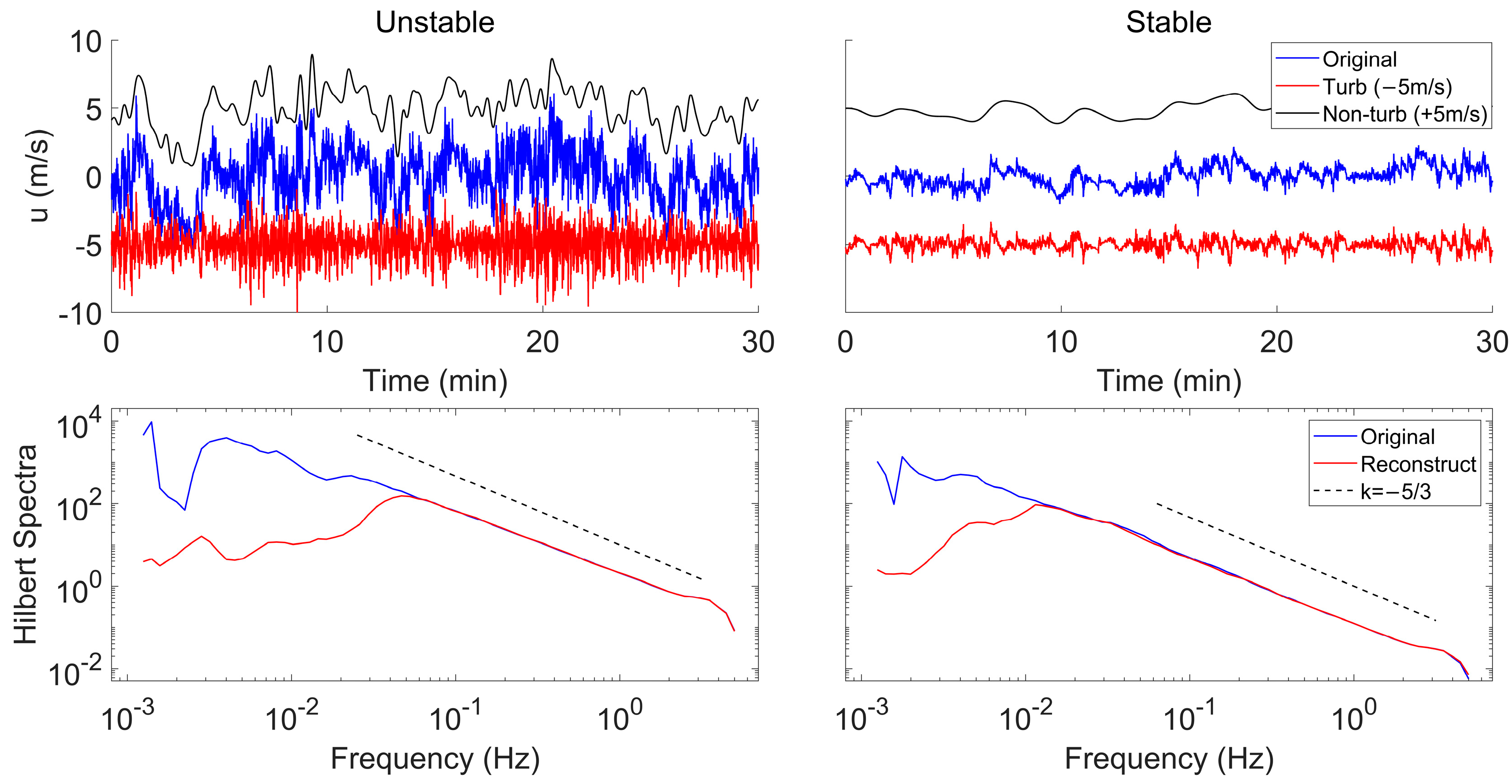
Figure 11 offers a comparative analysis of the time series and Hilbert spectra between the original and reconstructed u-wind in both stable and unstable cases. The time series elucidates that under stable stratification, both turbulent and non-turbulent motions exhibit mild behavior, with the amplitude of turbulent motion demonstrating significant variability. Conversely, under unstable stratification, both types of motions are more intense, characterized by larger average amplitudes and frequencies. In both scenarios, the non-turbulent motion significantly influences the shape of the time series. However, the boundary frequency in stable stratification tends to be smaller, indicative of the slow-changing features of non-turbulent motions. The Hilbert spectra reveals, from the energy point of view, that the non-turbulent motions of larger scales are eliminated, but there are still low-frequency components persisting. This is because the frequencies of IMFs are dynamic and time-dependent, and therefore reconstructing turbulence data by eliminating low-frequency IMFs will not result in a truncation in spectra like the filtering in Fourier spectra. The remaining low-frequency components share the same scale and dynamical properties as the motions in the sub-inertial range and thus do not disrupt the self-similarity characteristics of atmospheric turbulence.
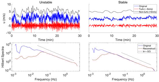
Figure 11.
The comparison of reconstructed and original turbulent time series of u-wind and their energy spectra. The left 2 panels for the unstable stratification case (10 July 09:00–09:30 LT), and the right ones for stable case (13 July 20:00–20:30 LT), LT = UTC + 8.
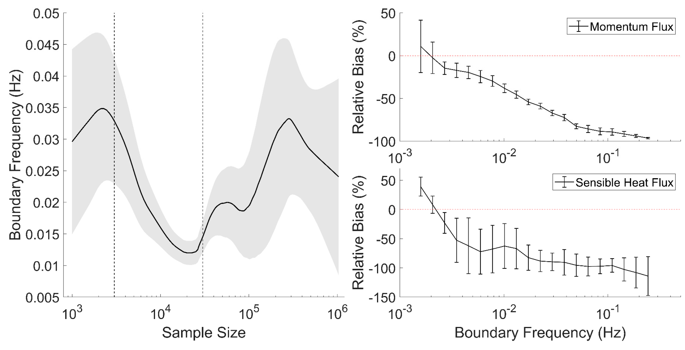
Similar to the fractal dimensions, the boundary frequency
is also dependent on the sample size. The left panel of Figure 12 depicts the relationship between boundary frequency and the sample size, which implies that
experiences three stages with the increase in sample size
:
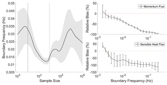
Figure 12.
Relationship between boundary frequency and the sample size (left) and the correction of turbulent momentum and sensible heat flux with respect to boundary frequency (right). The black dashed lines mark the division of different stages, the gray area and the error bars denote the 95% confidence intervals.
- (1)
- : the is higher and fluctuates with a large uncertainty; this is because not enough information is covered by the sample.
- (2)
- : the slightly decreases and reaches convergence, which means the turbulent properties are reflected by the sample and the can be effectively identified.
- (3)
- : the convergence of is broken, and the fluctuation becomes larger, which implies that the expanding of the sample makes large-scale motions blur the fractal dimensions and thus affect the estimation of .
From an application point of view, the turbulent momentum flux
and the sensible heat flux H defined by Equations (26) and (27) can be corrected through the reconstruction of turbulence data. The correction is quantified as the relative bias of the flux calculated from the reconstructed turbulent data and the original data (take sensible heat as an example):
In most cases, the turbulent flux (absolute value) of the reconstructed data is lower than that of the original data, suggesting an overestimation of the flux when non-turbulent motions are not eliminated. For the momentum flux, the correction spans from −100% to 0, with an average of approximately −50%, and the sensible heat flux exhibits a wider range of correction from −300% to +100%, with an average around −80%. Positive values of relative bias in turbulent fluxes correspond with the counter-gradient transport [64] of non-turbulent motion. However, this contributes more significantly to the gradient-wise transport, resulting in a general overestimation of the turbulent flux. The right two panels in Figure 12 reveal the relationship between relative bias and boundary frequency, which reflects that counter-gradient transport primarily occurs (albeit with a low confidence level) in instances where non-turbulent motions are mild and exhibit low frequencies, predominantly occurring in stable stratifications. As the boundary frequency increases, the trend shifts towards gradient-wise transport with increasing degrees of overestimation and decreasing degrees of uncertainties. This suggests that the overestimation of turbulent flux is a systematic issue that can be rectified through the application of fractal dimensions.
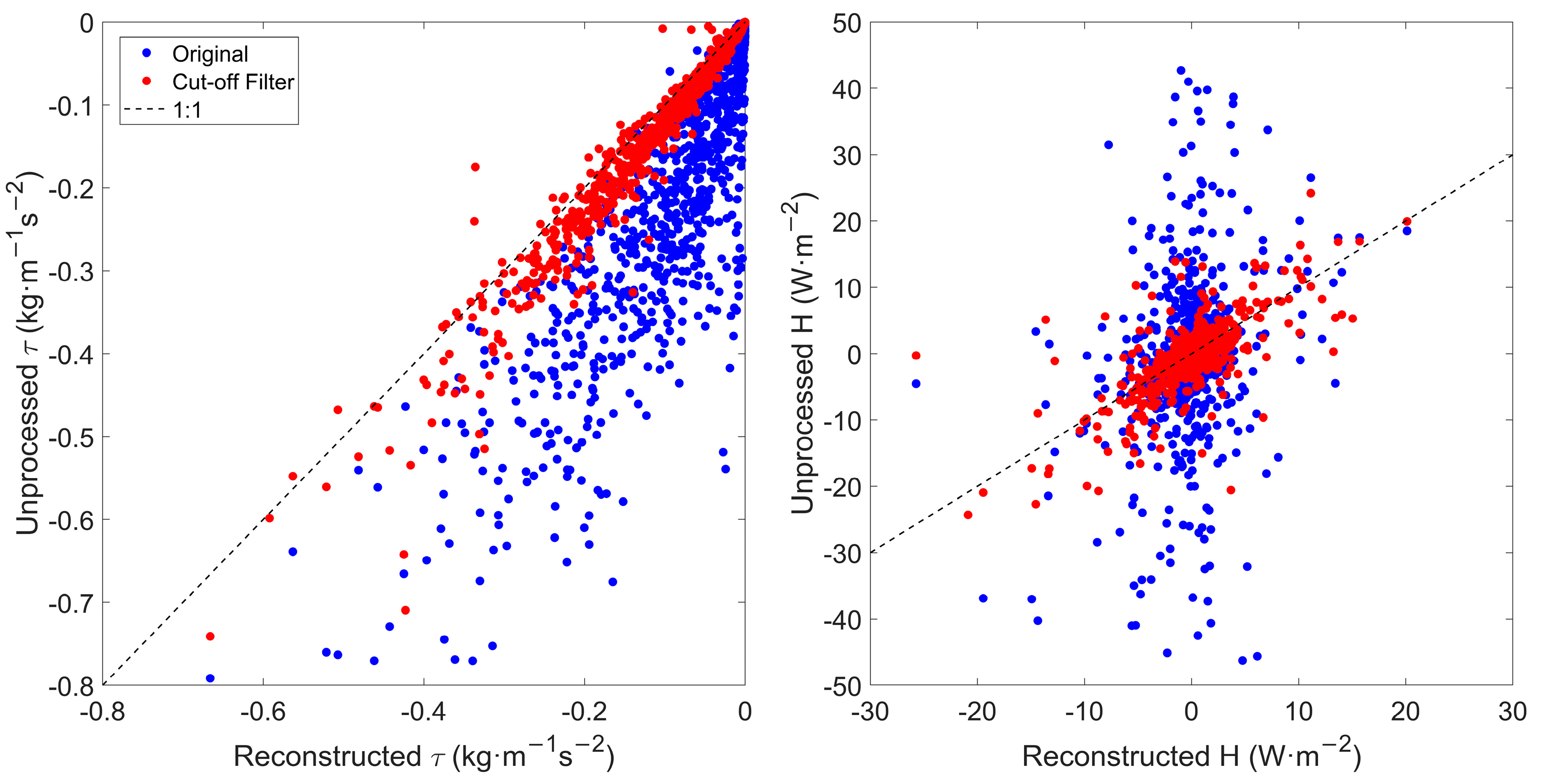
In the realm of practical applications, if the precise turbulent fluxes within a short time span are needed, they can be addressed through the application of the Hilbert–Huang transform. The algorithm shown in Figure 3 and Section 5.2 facilitates the elimination of non-turbulent motions with the aid of fractal dimensions, thereby enabling the computation of turbulent momentum and sensible heat fluxes. Figure 13 shows the comparison of the reconstructed fluxes and the unprocessed fluxes, which suggests that the reconstruction using Hilbert–Huang transform can relieve the overestimation of turbulent fluxes. Moreover, it is viable to summarize the relationship between boundary frequency and standard meteorological parameters; in this way, one can apply the high-pass filter and thereby separate turbulent motions at the boundary frequency in a more convenient way. However, the truncate way of processing the signal will result in the missing of physical components of turbulence, and therefore the effect of correction is less than the Hilbert–Huang transform. The results in this section may pave the way for the convenient correction of multiple turbulent flux samples.
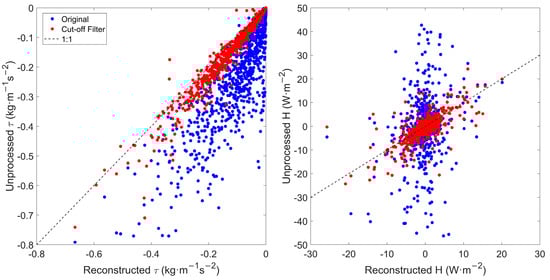
Figure 13.
Comparison of the reconstructed fluxes and the unprocessed fluxes in both July and December 2022. The red points show the fluxes estimated through cut-off filter of boundary frequencies, and the blue points the original fluxes.
Similar to the discussion in Section 4.2, it is also feasible to incorporate additional parameters such as potential temperature, CO2, and water vapor into the computation of fractal dimensions. By employing the generalized fractal dimensions, it becomes possible to reconstruct these variables along with their corresponding turbulent fluxes, yet the cost of computation can be higher. Therefore, if the calculation efficiency can be improved by advanced algorithms, such an approach will hold significant potential for parameterization schemes that involve turbulent fluxes. This could enhance the precision and effectiveness of simulations and models, thereby optimizing their performance in various applications. This represents a promising avenue for future research and development in this field.
6. Conclusions
As a natural dimensionless quantity, the fractal dimension can be instrumental in unveiling the chaotic and statistical properties of atmospheric turbulence. This study conducts an analysis of fractal dimensions from the 0th to the 2nd order with the aim of validating their potential through an examination of the properties of fractal dimensions and an exploration of their practical applications, including the identification of non-turbulent motions and the establishment of refined similarity relationships. The properties of fractal dimensions are scrutinized through an examination of the time series and similarity relationships. A comparative analysis of the time series of different orders of fractal dimensions reveals that these dimensions can reveal the properties of atmospheric turbulence, such as the diurnal pattern, the difference among seasons, and the occurrence of synoptic process. In different stratification conditions, the quasi-three-dimensional motion of atmospheric turbulence would be disturbed to different degree and decrease to near two-dimensional motion. Furthermore, the space distribution of fractal dimensions is revealed through the comparison of different heights, suggesting a scale-dependent nature of fractal dimensions. Based on the characteristics of fractal dimensions, two aspects of practical applications are investigated.
On one hand, the different orders of fractal dimensions can be taken into account in exploring new aspects of similarity relationships. It is tested that the ratio of 2nd and 0th orders fractal dimensions with respect to stability parameters shows a steady “1/3” exponential decreasing law, which can serve as the measure of multifractality. The multiplication of this ratio is demonstrated to be effective for both normalized standard deviation and cross-correlation coefficients. This enhances their distinguishability for different properties and increases their tolerance for errors, thereby reflecting the conditions of a broader range of atmospheric stratifications. It is conceivable that scalars, such as temperature and gas density, could also be considered as independent dimensions in the calculation of the fractal dimension. This holds the potential for further practical applications of fractal properties.
On the other hand, it is also believed that the properties of fractal dimensions can be further applied in the reconstruction of turbulence data and correction of turbulent fluxes. Given that motions of varying scales can significantly influence the value of fractal dimensions, it is possible to distinguish the motions with different contributions to the fractal dimension and thereby identify the non-turbulent part of motions in observational data. By locating the inflection point, the boundary frequency can be determined, which serves to identify the transition point of fractal properties. The sum of intrinsic mode functions below this boundary frequency is classified as non-turbulent motions, which can subsequently be eliminated in practice. The impact of fractal dimensions on the reconstruction of turbulence data can be substantiated through the calculation of turbulent flux. This aligns well with and mitigates the prevalent issue of overestimation of momentum and sensible heat flux.
The findings presented above reveal that the fractal dimensions and the conditions of atmospheric turbulence are closely related. This intimates the potential for broader application prospects that incorporate additional meteorological variables. Consequently, the analysis of fractal dimensions could offer substantial potential in enhancing the precision and effectiveness of parameterization schemes utilized in simulations and models concerning atmospheric boundary layers, and it suggests that the study of fractal dimensions could be a promising avenue for future research.
Author Contributions
Conceptualization, Z.L. and H.Z.; methodology, Z.L.; validation, Z.F.; formal analysis, Z.L.; resources, H.Z.; data curation, H.Z. and X.C.; writing—original draft preparation, Z.L.; writing—review and editing, H.Z., Z.F., X.C. and Y.S.; visualization, Z.L.; project administration, H.Z.; funding acquisition, H.Z. All authors have read and agreed to the published version of the manuscript.
Funding
This research was funded by National Key Research and Development Program of China, grant number 2023YFC3706300, and the National Natural Science Foundation of China, grant number 42175092, 92044301, and 91544216.
Data Availability Statement
Data used in this study are available from the corresponding author upon reasonable request (hsdq@pku.edu.cn).
Conflicts of Interest
The authors declare no conflicts of interest.
References
- Lorenz, E.N. Deterministic Nonperiodic Flow. J. Atmos. Sci. 1963, 20, 130–141. [Google Scholar] [CrossRef]
- Mandelbrot, B. How Long Is the Coast of Britain? Statistical Self-Similarity and Fractional Dimension. Science 1967, 156, 636–638. [Google Scholar] [CrossRef] [PubMed]
- Mandelbrot, B.B. The Fractal Geometry of Nature; Henry Holt and Company: New York, NY, USA, 1983. [Google Scholar]
- Falconer, K. Fractal Geometry: Mathematical Foundations and Applications; John Wiley & Sons Inc.: Hoboken, NJ, USA, 2003; pp. 1–26. [Google Scholar] [CrossRef]
- Garratt, J.R. Review: The Atmospheric Boundary Layer. Earth-Sci. Rev. 1994, 37, 89–134. [Google Scholar] [CrossRef]
- Kaimal, J.C.; Finnigan, J.J. Atmospheric Boundary Layer Flows: Their Structure and Measurement; Oxford University Press: Oxford, UK, 1994. [Google Scholar] [CrossRef]
- Sagan, H. Space-Filling Curves; Springer: New York, NY, USA, 1994; pp. 145–167. [Google Scholar] [CrossRef]
- Sharifi-Viand, A.; Mahjani, M.G.; Jafarian, M. Investigation of Anomalous Diffusion and Multifractal Dimensions in Polypyrrole Film. J. Electroanal. Chem. 2012, 67, 51–57. [Google Scholar] [CrossRef]
- Rényi, A. On the Dimension and Entropy of Probability Distributions. Acta Math. Hung. 1959, 10, 193–215. [Google Scholar] [CrossRef]
- Farmer, J.D.; Ott, E.; Yorke, J.A. The Dimension of Chaotic Attractors. Phys. D Nonlinear Phenom. 1983, 7, 153–180. [Google Scholar] [CrossRef]
- Grassberger, P.; Procaccia, I. Measuring the Strangeness of Strange Attractors. Phys. D Nonlinear Phenom. 1983, 9, 189–208. [Google Scholar] [CrossRef]
- Chhabra, A.; Jensen, R.V. Direct Determination of the f(α) Singularity Spectrum. Phys. Rev. Lett. 1989, 62, 1327–1330. [Google Scholar] [CrossRef] [PubMed]
- Roberts, A.J.; Cronin, A. Unbiased Estimation of Multi-Fractal Dimensions of Finite Data Sets. Phys. A Stat. Mech. Appl. 1996, 233, 867–878. [Google Scholar] [CrossRef]
- Posadas, A.N.D.; Giménez, D.; Bittelli, M.; Vaz, C.M.P.; Flury, M. Multifractal Characterization of Soil Particle-Size Distributions. Soil Sci. Soc. Am. J. 2001, 65, 1361–1367. [Google Scholar] [CrossRef]
- Alberti, T.; Consolini, G.; Ditlevsen, P.D.; Donner, R.V.; Quattrociocchi, V. Multiscale Measures of Phase-Space Trajectories. Chaos 2020, 30, 123116. [Google Scholar] [CrossRef] [PubMed]
- Hentschel, H.G.E.; Procaccia, I. The Infinite Number of Generalized Dimensions of Fractals and Strange Attractors. Phys. D Nonlinear Phenom. 1983, 8, 435–444. [Google Scholar] [CrossRef]
- de la Fuente Marcos, D.; de la Fuente Marcos, C. Multifractality in a Ring of Star Formation: The Case of Arp 220. Astron. Astrophys. 2006, 454, 473–480. [Google Scholar] [CrossRef]
- Trevino, J.; Liew, S.F.; Noh, H.; Cao, H.; Negro, L.D.; Structure, G. Multifractal Spectra and Localized Optical Modes of Aperiodic Vogel Spirals. Opt. Express 2012, 20, 3015–3033. [Google Scholar] [CrossRef]
- Gerges, F.; Geng, X.; Nassif, H.; Boufadel, M.C. Anisotropic Multifractal Scaling of Mount Lebanon Topography: Approximate Conditioning. Fractals 2021, 29, 2150112. [Google Scholar] [CrossRef]
- Ivanov, P.C.; Amaral, L.A.N.; Goldberger, A.L.; Havlin, S.; Rosenblum, M.G.; Struzik, Z.R.; Stanley, H.E. Multifractality in Human Heartbeat Dynamics. Nature 1999, 399, 461–465. [Google Scholar] [CrossRef] [PubMed]
- CIUCIU, P.; Varoquaux, G.; Abry, P.; Sadaghiani, S.; Kleinschmidt, A. Scale-Free and Multifractal Properties of Fmri Signals During Rest and Task. Front. Physiol. 2012, 3, 186. [Google Scholar] [CrossRef] [PubMed]
- Zorick, T.; Mandelkern, M.A. Multifractal Detrended Fluctuation Analysis of Human Eeg: Preliminary Investigation and Comparison with the Wavelet Transform Modulus Maxima Technique. PLoS ONE 2013, 8, e68360. [Google Scholar] [CrossRef]
- Saeedi, P.; Sorensen, S. An Algorithmic Approach to Generate after-Disaster Test Fields for Search and Rescue Agents. Lect. Notes Eng. Comput. Sci. 2009, 1, 93–98. [Google Scholar]
- Chen, Y. Modeling Fractal Structure of City-Size Distributions Using Correlation Functions. PLoS ONE 2011, 6, e24791. [Google Scholar] [CrossRef]
- Kamenshchikov, S.A. Transport Catastrophe Analysis as an Alternative to a Monofractal Description: Theory and Application to Financial Crisis Time Series. J. Chaos 2014, 2014, 346743. [Google Scholar] [CrossRef]
- Meneveau, C.; Sreenivasan, K.R. The Multifractal Nature of Turbulent Energy Dissipation. J. Fluid Mech. 1991, 224, 429–484. [Google Scholar] [CrossRef]
- Halsey, T.C.; Jensen, M.H.; Kadanoff, L.P.; Procaccia, I.; Shraiman, B.I. Fractal Measures and Their Singularities: The Characterization of Strange Sets. Phys. Rev. A 1986, 33, 1141–1151. [Google Scholar] [CrossRef] [PubMed]
- Benzi, R.; Biferale, L.; Paladin, G.; Vulpiani, A.; Vergassola, M. Multifractality in the Statistics of the Velocity Gradients in Turbulence. Phys. Rev. Lett. 1991, 67, 2299–2302. [Google Scholar] [CrossRef]
- Lovejoy, S.; Schertzer, D. The Weather and Climate: Emergent Laws and Multifractal Cascades; Schertzer, D., Lovejoy, S., Eds.; Cambridge University Press: Cambridge, UK, 2013; pp. 1–20. [Google Scholar] [CrossRef]
- Alberti, T.; Donner, R.V.; Vannitsem, S. Multiscale Fractal Dimension Analysis of a Reduced Order Model of Coupled Ocean–Atmosphere Dynamics. Earth Syst. Dyn. 2021, 12, 837–855. [Google Scholar] [CrossRef]
- Alberti, T.; Faranda, D.; Donner, R.V.; Caby, T.; Carbone, V.; Consolini, G.; Dubrulle, B.; Vaienti, S. Small-Scale Induced Large-Scale Transitions in Solar Wind Magnetic Field. Astrophys. J. Lett. 2021, 914, L6. [Google Scholar] [CrossRef]
- Carbone, F.; Alberti, T.; Faranda, D.; Telloni, D.; Consolini, G.; Sorriso-Valvo, L. Local Dimensionality and Inverse Persistence Analysis of Atmospheric Turbulence in the Stable Boundary Layer. Phys. Rev. E 2022, 106, 064211. [Google Scholar] [CrossRef] [PubMed]
- Altan, A.; Karasu, S.; Bekiros, S. Digital Currency Forecasting with Chaotic Meta-Heuristic Bio-Inspired Signal Processing Techniques. Chaos Solit. Fractals 2019, 126, 325–336. [Google Scholar] [CrossRef]
- Karasu, S.; Altan, A. Crude Oil Time Series Prediction Model Based on Lstm Network with Chaotic Henry Gas Solubility Optimization. Energy 2022, 242, 122964. [Google Scholar] [CrossRef]
- Özçelik, Y.B.; Altan, A. Overcoming Nonlinear Dynamics in Diabetic Retinopathy Classification: A Robust Ai-Based Model with Chaotic Swarm Intelligence Optimization and Recurrent Long Short-Term Memory. Fractal Fract. 2023, 7, 598. [Google Scholar] [CrossRef]
- Kolmogorov, A.N. Dissipation of Energy in Locally Isotropic Turbulence. Dokl. Akad. Nauk SSSR 1941, 32, 16. [Google Scholar]
- Monin, A.S.; Obukhov, A.M. Basic Laws of Turbulent Mixing in the Surface Layer of the Atmosphere. Akad. Nauk SSSR Geophiz. Inst. 1954, 24, 163–187. [Google Scholar]
- Foken, T. 50 Years of the Monin–Obukhov Similarity Theory. Bound.-Layer Meteorol. 2006, 119, 431–447. [Google Scholar] [CrossRef]
- Li, X.; Zhang, H. Size Distribution of Dust Aerosols Observed over the Horqin Sandy Land in Inner Mongolia, China. Aeolian Res. 2015, 17, 231–239. [Google Scholar] [CrossRef]
- Park, S.-U.; Park, M.-S. Aerosol Size Distributions Observed at Naiman in the Asian Dust Source Region of Inner Mongolia. Atmos. Environ. 2014, 82, 17–23. [Google Scholar] [CrossRef]
- Zhao, H.-L.; Zhou, R.-L.; Su, Y.-Z.; Zhang, H.; Zhao, L.-Y.; Drake, S. Shrub Facilitation of Desert Land Restoration in the Horqin Sand Land of Inner Mongolia. Ecol. Eng. 2007, 31, 1–8. [Google Scholar] [CrossRef]
- Vickers, D.; Mahrt, L. Quality Control and Flux Sampling Problems for Tower and Aircraft Data. J. Atmos. Ocean. Technol. 1997, 14, 512–526. [Google Scholar] [CrossRef]
- Huang, N.E.; Long, S.R.; Shen, Z. Advances in Applied Mechanics; Hutchinson, J.W., Wu, T.Y., Eds.; Elsevier: Amsterdam, The Netherlands, 1996; Volume 32, pp. 59C–117C. [Google Scholar] [CrossRef]
- Huang, N.E.; Shen, Z.; Long, S.R.; Wu, M.C.; Shih, H.H.; Zheng, Q.; Yen, N.-C.; Tung, C.C.; Liu, H.H. The Empirical Mode Decomposition and the Hilbert Spectrum for Nonlinear and Non-Stationary Time Series Analysis. Proc. R. Soc. A Math. Phys. Eng. Sci. 1998, 454, 903–995. [Google Scholar] [CrossRef]
- Huang, Y.X.; Schmitt, F.G.; Lu, Z.M.; Liu, Y.L. An Amplitude-Frequency Study of Turbulent Scaling Intermittency Using Empirical Mode Decomposition and Hilbert Spectral Analysis. Europhys. Lett. 2008, 84, 40010. [Google Scholar] [CrossRef]
- Rilling, G.; Flandrin, P.; Goncalves, P.; Lilly, J.M. Bivariate Empirical Mode Decomposition. IEEE Signal Process. Lett. 2007, 14, 936–939. [Google Scholar] [CrossRef]
- Rehman, N.; Mandic, D.P. Multivariate Empirical Mode Decomposition. Proc. R. Soc. A Math. Phys. Eng. Sci. 2010, 466, 1291–1302. [Google Scholar] [CrossRef]
- Rehman, N.; Mandic, D.P. Empirical Mode Decomposition for Trivariate Signals. IEEE Signal Process. Lett. 2009, 58, 1059–1068. [Google Scholar] [CrossRef]
- Wei, W.; Zhang, H.S.; Schmitt, F.G.; Huang, Y.X.; Cai, X.H.; Song, Y.; Huang, X.; Zhang, H. Investigation of Turbulence Behaviour in the Stable Boundary Layer Using Arbitrary-Order Hilbert Spectra. Bound.-Layer Meteorol. 2017, 163, 311–326. [Google Scholar] [CrossRef]
- Ren, Y.; Zhang, H.; Wei, W.; Wu, B.; Cai, X.; Song, Y. Effects of Turbulence Structure and Urbanization on the Heavy Haze Pollution Process. Atmos Chem. Phys. 2019, 19, 1041–1057. [Google Scholar] [CrossRef]
- Huang, Y.X.; Schmitt, F.G.; Lu, Z.M.; Fougairolles, P.; Gagne, Y.; Liu, Y.L. Second-order structure function in fully developed turbulence. Phys. Rev. E 2010, 82, 026319. [Google Scholar] [CrossRef]
- Huang, N.E.; Wu, Z. A Review on Hilbert-Huang Transform: Method and Its Applications to Geophysical Studies. Rev. Geophys. 2008, 46, RG2006. [Google Scholar] [CrossRef]
- Senroy, N. Inter-Area Oscillations in Power Systems: A Nonlinear and Nonstationary Perspective; Messina, A.R., Ed.; Springer: Boston, MA, USA, 2009; pp. 37–61. [Google Scholar]
- Wu, Z.; Huang, N.E. Ensemble Empirical Mode Decomposition: A Noise-Assisted Data Analysis Method. Adv. Adapt. Data Anal. 2009, 1, 1–41. [Google Scholar] [CrossRef]
- Yeh, J.; Shieh, J.; Huamg, N. Complementary Ensemble Empirical Mode Decomposition: A Novel Noise Enhanced Data Analysis Method. Adv. Adapt. Data Anal. 2010, 2, 135–156. [Google Scholar] [CrossRef]
- De Bruin, H.A.R.; Kohsiek, W.; Van Den Hurk, B.J.J.M. A Verification of Some Methods to Determine the Fluxes of Momentum, Sensible Heat, and Water Vapour Using Standard Deviation and Structure Parameter of Scalar Meteorological Quantities. Bound.-Layer Meteorol. 1993, 63, 231–257. [Google Scholar] [CrossRef]
- Quan, L.; Hu, F. Relationship between Turbulent Flux and Variance in the Urban Canopy. Meteorol. Atmos. Phys. 2009, 104, 29–36. [Google Scholar] [CrossRef]
- Wood, C.R.; Lacser, A.; Barlow, J.F.; Padhra, A.; Belcher, S.E.; Nemitz, E.; Helfter, C.; Famulari, D.; Grimmond, C.S.B. Turbulent Flow at 190 m Height above London During 2006–2008: A Climatology and the Applicability of Similarity Theory. Bound.-Layer Meteorol. 2010, 137, 77–96. [Google Scholar] [CrossRef]
- Sreenivasan, K.R.; Prasad, R.R.; Meneveau, C.; Ramshankar, R. The Fractal Geometry of Interfaces and the Multifractal Distribution of Dissipation in Fully Turbulent Flows. Pure Appl. Geophys. 1989, 131, 43–60. [Google Scholar] [CrossRef]
- Vassilicos, J.C.; Hunt, J.C.R. Fractal Dimensions ansd Spectra of Interfaces with Application to Turbulence. Proc. Math. Phys. Sci. 1991, 435, 505–534. [Google Scholar] [CrossRef]
- Carbone, F.; Alberti, T.; Sorriso-Valvo, L.; Telloni, D.; Sprovieri, F.; Pirrone, N. Scale-Dependent Turbulent Dynamics and Phase-Space Behavior of the Stable Atmospheric Boundary Layer. Atmosphere 2020, 11, 428. [Google Scholar] [CrossRef]
- Mahrt, L. Characteristics of Submeso Winds in the Stable Boundary Layer. Bound.-Layer Meteorol. 2009, 130, 1–14. [Google Scholar] [CrossRef]
- Mahrt, L. Variability and Maintenance of Turbulence in the Very Stable Boundary Layer. Bound.-Layer Meteorol. 2010, 135, 1–18. [Google Scholar] [CrossRef]
- Vickers, D.; Mahrt, L. A Solution for Flux Contamination by Mesoscale Motions with Very Weak Turbulence. Bound.-Layer Meteorol. 2006, 118, 431–447. [Google Scholar] [CrossRef]


Disclaimer/Publisher’s Note: The statements, opinions and data contained in all publications are solely those of the individual author(s) and contributor(s) and not of MDPI and/or the editor(s). MDPI and/or the editor(s) disclaim responsibility for any injury to people or property resulting from any ideas, methods, instructions or products referred to in the content. |
© 2024 by the authors. Licensee MDPI, Basel, Switzerland. This article is an open access article distributed under the terms and conditions of the Creative Commons Attribution (CC BY) license (https://creativecommons.org/licenses/by/4.0/).