Dynamical Behavior of the Fractional BBMB Equation on Unbounded Domain

Abstract

The fractional-order Benjamin-Bona-Mahony-Burgers (BBMB) equation is a generalization of the classical BBMB equation. It’s dynamic behaviors is much more complex than that of the corresponding integer-order BBMB equation. The main purpose of this paper is to explore the dynamic behaviors of the fractional-order BBMB equations by using the Fourier spectral method. Firstly, the numerical solution is compared with the exact solution. It is proved that the proposed method is effective and high precision for solving the spatial fractional order BBMB equation. Then, some dynamical behaviors of fractional order BBMB equations are obtained by using the present method, and some novel fractal waves of the the fractional-order BBMB equation on unbounded domain are shown.

1. Introduction

Fractional calculus [1,2,3] is often considered a generalization of integral calculus. Because of its wide application in the field of science and engineering, it has aroused great interest. The fractional-order BBMB equation is a mathematical model that generalizes the classical BBMB equation by incorporating fractional-order derivatives. This equation is significant for the correct description of physical problems involving long waves in nonlinear dispersive media, such as water waves, where the classical integer-order models may not accurately capture the dynamics of the system. The fractional-order derivatives provide a more refined representation of the memory and hereditary properties of the medium, leading to a better approximation of the dispersion and dissipation effects. The fractional-order BBMB equation is particularly useful in situations where the wave propagation exhibits nonlocality and non-linearity, and it can model the unidirectional wave behavior more accurately than the classical models. It has been applied to various fields, including fluid dynamics, where it helps in understanding wave interactions, wave energy transfer, and wave breaking phenomena. The dynamic behavior of the fractional-order BBMB equation is much more complex than that of corresponding integer-order BBMB equation. The exact solution of fractional-order BBM equation is not easy to obtain. Therefore, numerical calculation becomes the first choice for studying fractional order BBM equations.

In order to explore the dynamic behavior of the BBMB equation, various numerical methods have been proposed. In [4], a fourth-order B-spline collocation method is used to get the solution of the BBMB equation. In the quasi-linearization process, the time domain is discretized by Crank-Nicolson scheme to deal with nonlinear terms. The simple cubic B-spline collocation method is used for spatial discretization. In [5], a meshless numerical scheme based on finite difference method and Kansa-radial basis function to solve the fractional-in time Oskolkov BBMB equation. The time fractional derivative is discretized by finite difference scheme, and then the space derivative is discretized by Kansa method. In [6], a generalized time-fractional BBMB equation with ABC derivative is solved. The method applied linearization technique to discretize nonlinear expressions, using Crank-Nicolson scheme in time direction and central difference scheme in space direction. In [7], the homotopy analysis method [8,9] is used to solve the the fractional BBMB equation. In [10], a pseudo-spectral method based on the Chebyshev cardinal functions is used to solve the fractional BBMB equation with a local variable-order conformable fractional derivative numerically. The numerical comparison with the cubic B-spline method and the hybrid method generated of the the quintic Hermite method and the finite difference method is made to determine the effectiveness of the pseudo-spectral method. In [11], the cubic B-spline basis function is used to solve the fractional BBMB equation with the Caputo fractional derivative. It’s main idea is the time and space derivatives are interpolated by forward finite difference scheme and the Crank-Nicolson scheme combined with B-spline basis function. In [12], a second-order predictor-corrector method is proposed for the fractional BBMB equations with weak singularity at the initial time.

Since fractional BBMB equations usually do not have available analytical solutions, numerical methods play an important role in the practical testing and application of these models. Unlike integer derivatives, fractional derivatives have weak singularity, non-locality, and sometimes even spatio-temporal coupling, which brings many difficulties and challenges to the design, analysis and implementation of numerical methods. Therefore, although the numerical solution of fractional BBMB equation has received a lot of attention and made a lot of progress in recent decades, it is still a dynamic discipline, and there are still many problems to be solved.

In recent years, infinite dimensional dynamical systems have been greatly developed. With the deepening of its research and the rapid improvement of computers, the numerical research methods related to it have been paid more and more attention. As a numerical method for solving partial differential equations, spectral method has infinite order convergence. Therefore, spectral methods have attracted more attention. The Fourier spectral method (FSM) is an effective method for solving partial differential equations numerically [13]. The idea of the FSM is: firstly, the fast Fourier transform (FFT) of partial differential equations is performed to obtain a ordinary differential equations with time variable. Then, a numerical scheme based on time steps is used to solve this system of the ordinary differential equations. Because the fractional-order differential model has the advantages of memory effect and heredity in describing the dynamic behavior of the system, the study of the solution of fractional-order differential equation is a hot issue [14,15].

The goal of this paper is to investigated of dynamical behavior variation of the fractional BBMB equation on unbounded domain, and to discover some novel dynamic behavior the fractional BBMB equation on unbounded domain.

2. Description of Method

The fractional BBMB equation is a generalization of the classical BBMB equation, which is used to model long internal waves in a stratified fluid, such as shallow water waves. The fractional-order version of the equation incorporates memory effects and is represented using fractional derivatives, which provide a more accurate description of the underlying physical phenomena. This paper considers the following fractional BBMB equation [16,17]:

$$\left\{\begin{array}{c}{u}_t+a{D}_x^{\alpha }u+b{u}^{p-1}{u}_x-c{u}_{xx}-d{u}_{xxt}=0,(x,t)\in R\times [0,T],\hfill \\ u(x,0)=u_0\left(x\right),x\in R,\hfill \\ \left|u\right(x,t\left)\right|\to 0,\left|x\right|\to \infty ,0<t\le T,\hfill \end{array}\right.$$

(1)

where $\alpha$, a, $b,c,d$ and p are constants, $0<\alpha \le 1$, $D_x^{\alpha }u$ represents Caputo fractional derivative operator.

When $\alpha =a=b=d=1,c=0,p=2$, Equation (1) is known as the Benjamin-Bona-Mahony equation [16], which has the following form

$$u_t+u_x+u{u}_x-u_{xxt}=0.$$

(2)

The Benjamin-Bona-Mahony equation [18,19] is also called as the regularized long wave equation, it’s describes the unidirectional wave propagation of long waves with small amplitudes in a medium, which is of great importance in physics.

When $\alpha =a=b=d=1,p=2$, Equation (1) is known as the BBMB equation [20].

$$u_t+u_x+u{u}_x-c{u}_{xx}-u_{xxt}=0.$$

(3)

Applying the fast Fourier transform in both sides of (1) for spatial variable x, Equation (1) can be transformed into the following ODEs:

$$\frac{d\widehat{u}}{dt}(\omega ,t)=\left(-(a{\left(i\omega \right)}^{\alpha }+c{\omega }^2)\widehat{u}(\omega ,t)-b{F}_x(u^{p-1}{u}_x\right))/\left(1+d{\omega }^2\right).$$

(4)

where the discrete FFT of function $u(x,t)$ about x and inverse discrete FFT of function $\widehat{u}(\omega ,t)$ about $\omega$ are

$$\begin{array}{c}\widehat{u}\left(\omega ,t\right)=F_x\left(u\right)=\frac{1}{K}{\displaystyle \sum _{j=0}^{K-1}}u\left(x_j,t\right)e^{-i\omega x_j},-\frac{K}{2}\le \omega \le \frac{K}{2}-1,\hfill \\ u\left(x,t\right)=F_{\omega }^{-1}\left(\widehat{u}\right)={\displaystyle \sum _{\omega =-\frac{K}{2}}^{\frac{K}{2}-1}}\widehat{u}\left(\omega ,t\right)e^{i\omega x_j},0\le j\le K-1.\hfill \end{array}$$

(5)

In calculation, we call the function fftshift in MATLAB. Then, the Runge-Kutta method is used to solve (4), and form

$$\left\{\begin{array}{cc}& {\widehat{u}}_{n+1}={\widehat{u}}_n+\frac{h}{6}({\mathbf{k}}_{\mathbf{1}}+2{\mathbf{k}}_{\mathbf{2}}+2{\mathbf{k}}_{\mathbf{3}}+{\mathbf{k}}_{\mathbf{4}}),\hfill \\ & {\mathbf{k}}_{\mathbf{1}}=g(t_n,{\widehat{u}}_n),\hspace{1em}\hspace{1em}{\mathbf{k}}_{\mathbf{2}}=g(t_n+\frac{h}{2},{\widehat{u}}_n+\frac{h{\mathbf{k}}_{\mathbf{1}}}{2}),\hfill \\ & {\mathbf{k}}_{\mathbf{3}}=g(t_n+\frac{h}{2},{\widehat{u}}_n+\frac{h{\mathbf{k}}_{\mathbf{2}}}{2}),\hspace{1em}\hspace{1em}{\mathbf{k}}_{\mathbf{4}}=g(t_n+h,{\widehat{u}}_n+h{\mathbf{k}}_{\mathbf{3}}),\hfill \end{array}\right.$$

where $g(t,\widehat{u})=\left(-(a{\left(i\omega \right)}^{\alpha }+c{\omega }^2)\widehat{u}(\omega ,t)-b{F}_x(u^{p-1}{u}_x\right))/\left(1+d{\omega }^2\right),h$ is step-size. The convergence and error analyses of the method see Ref. [21].

3. Numerical Experiment

Next, we perform numerical experiments. Firstly, the numerical solution of the present method is compared with the exact solution and with the numerical solution of other methods [20,22,23,24,25,26] to determine the validity of the present method. Spatial domain is $x\in [\frac{-L}{2},\frac{L}{2}]$, space step length is $L/N$, time step is h.

Experiment 1.

Considering the Equation (1) with $\alpha =a=b=1$, $c=d=0$, $p=2$ and the following initial conditions

$$u(x,0)=3c{sec}^2\left(kx\right),x\in [-80,80]$$

The exact solution is $u(x,t)=3c{sec}^2(kx-kvt)$. It has amplitude $3c$, width $k=\sqrt{\frac{c}{4v}}$, and wave velocity $v=1+c$.

First of all, when $c=0.1$, we compare the infinite norm of errors under different methods in Table 1. Table 2 shows the $L_{\infty }$ of errors when $c=0.03$. We can directly observe from the table that the error of the method used in this paper is the smallest, reaching ${10}^{-7}$, which also demonstrates the accuracy and effectiveness of the present method.

Table 1. Comparison of $L_{\infty }$ error at $c=0.1$ for Experiment 1.

t	Algorithm in [22]	Finite Element Method [22]	Cubic B-Spline Method [20]	Present Method
2	6.8170 × 10−3	9.0000 × 10−6	3.5753 × 10−6	1.7367 × 10−7
4	1.3740 × 10−2	1.7000 × 10−5	5.9568 × 10−6	1.9645 × 10−7
6	2.0710 × 10−2	2.6000 × 10−5	8.4798 × 10−6	4.1904 × 10−7
8	2.7660 × 10−2	3.6000 × 10−5	1.0519 × 10−5	3.8485 × 10−7
10	3.4550 × 10−2	4.4000 × 10−5	1.2062 × 10−5	4.6152 × 10−7

Table 2. Comparison of $L_{\infty }$ error at $c=0.03$ for Experiment 1.

t	Algorithm in [22]	Finite Element Method [22]	Cubic B-Spline Method [20]	Present Method
2	3.9200 × 10−4	2.7400 × 10−4	2.7430 × 10−4	6.9387 × 10−6
4	7.8600 × 10−4	2.3000 × 10−4	2.2998 × 10−4	1.8324 × 10−5
6	1.1830 × 10−3	2.2500 × 10−4	2.2498 × 10−4	3.3104 × 10−5
8	1.5820 × 10−3	2.2100 × 10−4	2.2103 × 10−4	5.0898 × 10−5
10	1.9830 × 10−3	2.1700 × 10−4	2.1676 × 10−4	7.3263 × 10−5

From Figure 1, we can clearly see the shape of solitary wave solution in Experiment 1. From Figure 1c, we can also see that the error is relatively large at $x=0$ and the boundary. Figure 2 contains the contour map and density map of $c=0.1$. From Figure 1 and Figure 2, we find that the value of the function value at near $x=0$ is relatively large, and the function value at the boundary tends to be zero.

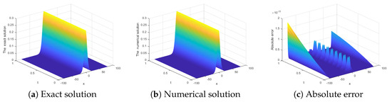
Figure 1. Comparison the exact solution with the numerical solution of Experiment 1 at $t=1,c=0.1,\tau =0.001,L=160,N=1024$.

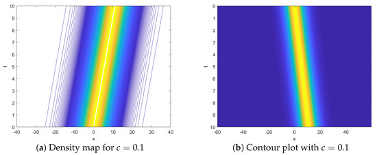
Figure 2. Contour plot and density plot with $c=0.1$,$\tau =0.001,L=160,N=1024$.

We show logarithmic of absolute error of Experiment 1 at different time t and c in Figure 3 and Figure 4. From Figure 3 and Figure 4, we find that the solution is stable at different times. We also find that L also affects the error of the function, and the error will increase with the increase of c. From Table 3, we find that the conservation laws in this paper is more accurate than that in other articles, this also emphasizes the effectiveness of the present method.

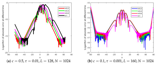
Figure 3. Logarithmic of absolute error of Experiment 1 at different time t and c.

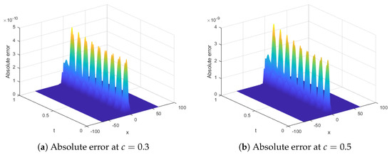
Figure 4. Absolute error of Experiment 1 at $t=1,\tau =0.001,L=128,N=1024$.

Table 3. Comparison of the conservation laws with $N=1024$ and $c=0.1$ for Experiment 1.

Method	$\mathit{\tau }$	${\mathit{C}}_1$	${\mathit{C}}_2$	${\mathit{C}}_3$
Analytical		3.9799497	0.81046249	2.579007
Present method	0.01	3.9799497	0.81046249	2.579007
Method I in [23]	0.01	3.9799	0.8104	2.5790
Method II in [23]	0.01	3.9799	0.8104	2.5790
Method in [24]	0.01	3.97988	0.810453	2.57898

Where conservation laws is the following form:

$$\begin{array}{c}\hfill \begin{array}{c}{C}_1=h{\displaystyle \sum _{j=1}^N}{u}_j^n,C_2=h{\displaystyle \sum _{j=1}^N}[{\left(u_j^n\right)}^2+b{\left({\left(u_x\right)}_j^n\right)}^2],C_3=h{\displaystyle \sum _{j=1}^N}[{\left(u_j^n\right)}^3+3{\left(u_j^n\right)}^2].\hfill \end{array}\end{array}$$

where $u_j^n$ stands for $u(x_j,t_n)$, $h=\frac{L}{N}$.

Figure 5 compares the numerical solution and the exact solution, and shows absolute error of $c=0.03$. We find that the absolute error can still be very small for a long time. Figure 6 shows logarithmic of absolute error of Experiment 1 at $c=0.1,\tau =0.001,L=120,N=1024$, and confirms the stability of the solution by observing the two errors of $c=0.05$ and $0.03$. From Figure 5 and Figure 6, we verify the effectiveness and accuracy of our method, and the above conclusions are still valid for a long time.

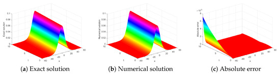
Figure 5. Numerical results of Experiment 1 at $t=1,c=0.03,\tau =0.001,L=160,N=1024$.

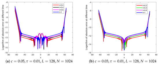
Figure 6. Logarithmic of absolute error of Experiment 1 at $c=0.1,\tau =0.001,L=120,N=1024$.

Next, we want to explore the solution of the fractional BBMB equation. Because it is difficult to obtain an analytical solution for the fractional BBMB Equation (1), so we can use the present method to study the numerical solution of confirmed. In Figure 7, We show some numerical solutions at different fractional derivative $\alpha =0.7,0.8,0.9,$ for Experiment 1. From Figure 7, we can observe that the shapes of the three Figures are similar. The closer $\alpha$ is to 1, the more its soliton wave is consistent with the soliton wave of $\alpha =1$.

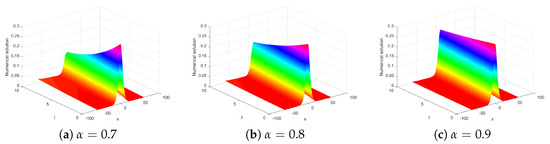
Figure 7. Numerical solutions of Experiment 1 with different $\alpha$ at $t=1,\tau =0.001,L=120,N=1024$.

Subsequently, In Figure 8, we fixed the value of x and explored the influence of different $\alpha$ on the function u. We found that the function decreases with the transformation of t at $x=0$, but when $x=10$, the change of u is opposite. In Figure 9, we find that the peak of u is increases with the increase of A, and the value of T also affects the position of the peak, but the shape of the wave is bounded since stability is a property of the system rather than a property of a signal. At the same time, we also notice that the amplitude $3c$ also affects the peak value.

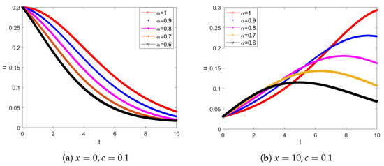
Figure 8. Propagation of wave at different $\alpha$ at $x=0,10$ when $c=0.1$ for Experiment 1.

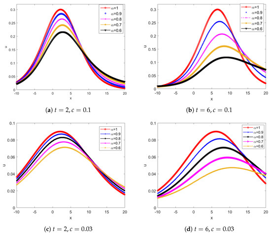
Figure 9. Propagation of wave at $\alpha ,t=2,6$, $c=0.1,0.03$ for Experiment 1.

Experiment 2.

Considing the fractional BBMB equation with $b=p=4,\alpha =1$, $c=d=0$ and $b=p=8,\alpha =1$, $c=0$, with the following initial condition

$$u(x,0)={\left(\frac{p+1}{3}\right)}^{\frac{1}{p-1}}{sec}^{\frac{2}{p-1}}\left(kx\right),\hspace{1em}\hspace{1em}x\in [-50,50].$$

The exact solution is $u(x,t)=A{sec}^{\frac{2}{p-1}}(kx-kvt).$ It has amplitude $A={\left[\frac{(p+1)(v-1)}{2}\right]}^{\frac{1}{p-1}}$, and $k=\frac{p-1}{2}\sqrt{\frac{}{}}v-1v$.

In this Experiment, In order to clarify the validity of the present method on the unbounded domain $\left|u\right(x,t\left)\right|\to 0,\left|x\right|\to \infty ,0<t\le T$, we set the parameters $v=\frac{4}{3}$ and $\tau =0.01$, $L=1024\times 8,N=1024\times 8$. Comparison of numerical and exact solutions at $p=4$ for Experiment 2 is shown in Figure 10. We set the parameters $v=\frac{4}{3}$ and $\tau =0.01$, $L=100$, $N=1024$. Comparisons of numerical and exact solutions at $t=0.1,p=4$ and $p=8$ for Experiment 2 are shown in Table 4. Comparisons of $L_{\infty }$ error for Example 2 are shown in Table 5. From Table 4 and Table 5, we find that the error of the method is the smallest compared with other methods, which again shows the effectiveness of the method. Absolute error of Experiment 2 with $p=4,8$ at $t=1,\tau =0.001,L=100,N=1024$ is shown in Figure 11.

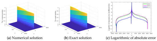
Figure 10. Comparison the exact solution with the numerical solution of Experiment 1 at $t=1,p=4,L=1024\times 8;N=1024\times 8$.

Table 4. Comparison of the numerical solution of the present with the exact solution at $t=0.1,p=4$ and $p=8$ for Experiment 2.

p	x	Exact Solution	Numerical Solution	Absolute Error
4	−10	0.0094	0.0094	2.3306 × 10−12
	−5	0.1147	0.1147	7.3283 × 10−11
	0	0.9379	0.9379	1.5064 × 10−9
	5	0.1310	0.1310	1.8122 × 10−10
	10	0.0108	0.0108	3.5643 × 10−12
8	−10	0.0081	0.0081	2.5062 × 10−12
	−5	0.0992	0.0992	3.3017 × 10−10
	0	1.0515	1.0515	2.5424 × 10−9
	5	0.1133	0.1133	2.2898 × 10−10
	10	0.0093	0.0093	2.0325 × 10−12

Table 5. Comparison of $L_{\infty }$ error for Experiment 2.

p	t	Finite Difference Scheme [25]	Finite Difference Scheme [26]	Present Method
4	0.2	2.3111 × 10−3	2.4126 × 10−3	4.5129 × 10−9
	0.4	4.7384 × 10−3	4.9448 × 10−3	4.9426 × 10−9
	0.6	7.1138 × 10−3	7.4230 × 10−3	5.9942 × 10−9
	0.8	9.2928 × 10−3	9.7015 × 10−3	6.9753 × 10−9
	1.0	1.1261 × 10−2	1.1760 × 10−2	5.6849 × 10−9
8	0.2	1.1151 × 10−2	1.1290 × 10−2	7.5195 × 10−8
	0.4	2.1295 × 10−2	2.2573 × 10−2	1.8036 × 10−7
	0.6	3.1416 × 10−2	3.2822 × 10−2	2.8450 × 10−7
	0.8	4.1946 × 10−2	4.2464 × 10−2	3.8517 × 10−7
	1.0	5.0220 × 10−2	5.1841 × 10−2	4.8838 × 10−7

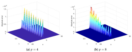
Figure 11. Absolute error of Experiment 2 with $p=4,8$ at $t=1,\tau =0.001,L=100,N=1024$.

Experiment 3.

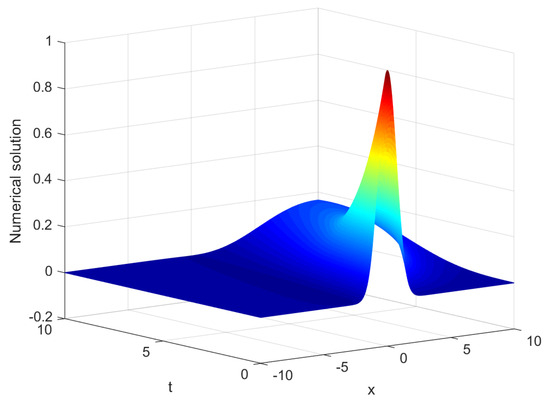
Next, we will give some numerical solutions. Now let’s consider the fractional BBMB Equation (1), the initial condition is $u(x,0)=e^{-x^2}$, the parameters are $a=b=\alpha =1,p=2,c=1$. It is difficult to get the exact solution of the fractional BBMB equation. Now we get the numerical solution. The numerical solution see Figure 12, Figure 13, Figure 14 and Figure 15.

Figure 12. Numerical solution at $u(x,0)=e^{-x^2}$ for Experiment 3.

Figure 13. Density map at $u(x,0)=e^{-x^2}$ for Experiment 3.

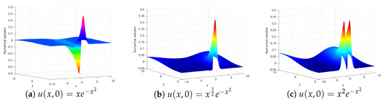
Figure 14. Numerical solution for Experiment 3 with different initial condition at $\tau =0.001,L=20,N=1024$.

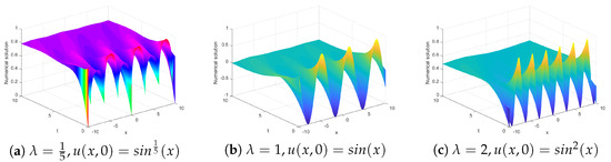
Figure 15. Numerical solutions of Experiment 3 with different initial conditioat $\tau =0.001,L=20,N=1024$.

Next, we give the numerical solution of the fractional BBMB equation at different initial conditions. First, we study the fractional BBMB equation with initial condition $u(x,0)=x{e}^{-x^2}$, $u(x,0)=x^{\frac{3}{2}}{e}^{-x^2}$ and $u(x,0)=x^2{e}^{-x^2}$, we get the numerical solution in Figure 14. We observe that the number of wave peaks in these three pictures is different at $t=0$. The Figure 14a has two upward and downward peaks, the Figure 14b has only one peak, and the Figure 14c has two upward peaks.

In order to further study the influence of the initial problem on the equation, we consider the initial conditions $u(x,0)=si{n}^{\lambda }\left(x\right)$ of the fractional BBMB Equation (1) with $a=b=\alpha =1,p=2,c=1,d=0$, Figure 15 shows The numerical results at $\tau =0.001,L=20,N=1024$ and the initial conditions are $u(x,0)=si{n}^{\lambda }\left(x\right)$, we can observe that the numerical solution fluctuates greatly at $t=0$.

Experiment 4.

Considing the undular bore solution of the fractional BBMB Equation (1) with initial conditions $u(x,0)=0.05[1-tanh\left(\frac{x}{d}\right)]$ and $a=\alpha =1,p=2,b=1.5,c=0,d=\frac{1}{6}$.

Figure 16, Figure 17, Figure 18 and Figure 19 show the numerical solution of $u(x,t)$. Figure 18 and Figure 19 show undulation profiles for the gentle slope at $d=2$, $t=100$ and $t=250$ for Experiment 4. Figure 18 and Figure 19 are in perfect agreement with those in reference [27].

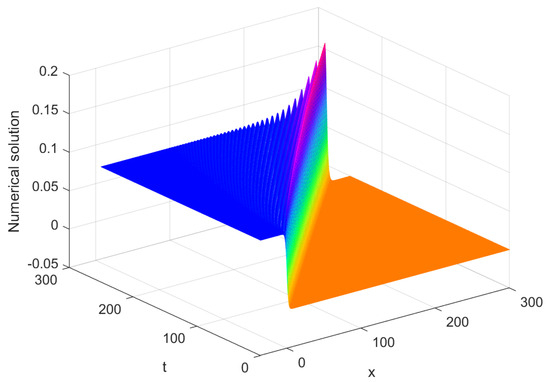
Figure 16. Three-dimensional diagram for numerical solution of Experiment 4.

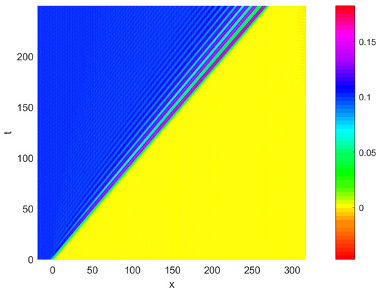
Figure 17. Graph of numerical solution of Experiment 4.

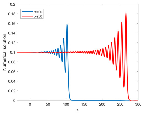
Figure 18. Undulation profiles for the gentle slope $d=2$ at $t=100$ and $t=250$ of Experiment 4.

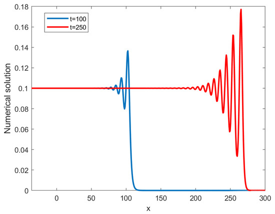
Figure 19. Undulation profiles for the gentle slope $d=5$ at $t=100$ and $t=250$ of Experiment 4.

The Fourier spectral method is particularly suitable for dealing with periodic boundary conditions because it can naturally deal with periodic problems. For aperiodic boundary conditions, Experiment 4 also shows valid numerical results. It’s just a special case. In general, for aperiodic boundary conditions, it may be necessary to use more complex techniques, such as a combination of spectral methods with boundary element methods, or to use specific processing techniques near the boundary.

4. Conclusions

This paper presents a detailed study on the dynamic behavior of the fractional-order BBMB equation using the Fourier spectral method, and some novel fractal waves of the the fractional-order BBMB equation on unbounded domain are shown. Through a series of numerical experiments, we have successfully demonstrated the effectiveness and accuracy of their proposed method in solving the space in fractional BBMB equation. The research has unveiled novel fractal wave propagation behaviors, which are more complex than those of the integer-order BBMB equation. The findings indicate that as the fractional parameter $\alpha$ approaches 1, the solution of the fractional BBMB equation converges to the classical solution, showcasing the method’s robustness and reliability across various spatial domains and parameter values. It was observed that as $\alpha \to 1$, the approximation solution increasingly overlaps with classical solutions visually and through tabular data. The behavior of traveling waves was studied across different domains of x, revealing improved solution profiles and smoother waves with extended domains. The influence of fractional parameter $\alpha$ on various spatial ranges was investigated, showing varying wave patterns for smaller values before smoothing out at larger values. Stability analysis revealed that the suggested scheme is unconditionally stable. Error norms for different domains of x were presented in table form, indicating suitability for any domain.

The findings are expected to contribute to a deeper understanding of wave interactions, energy transfer, and wave breaking phenomena in nonlinear dispersive media, with potential applications in fluid dynamics and other scientific fields. In the future, we will continue to explore the interesting dynamic behavior [28,29] of other fractional differential equations.

References

- Daftardar-Gejji, V. (Ed.) Fractional Calculus and Fractional Differential Equations; Springer: Singapore, 2019. [Google Scholar]
- Li, Z.; Chen, Q.; Wang, Y.; Li, X. Solving two-sided fractional super-diffusive partial differential equations with variable coefficients in a class of new reproducing kernel spaces. Fractal Fract. 2022, 6, 492. [Google Scholar] [CrossRef]
- Li, C.P.; Li, Z.Q. The blow-up and global existence of solution to Caputo-Hadamard fractional partial differential equation with fractional Laplacian. J. Nonlinear Sci. 2021, 31, 80. [Google Scholar] [CrossRef]
- Kukreja, V.K. Numerical treatment of Benjamin-Bona-Mahony-Burgers equation with fourth-order improvised B-spline collocation method. J. Ocean Eng. Sci. 2022, 7, 99–111. [Google Scholar]
- Sagar, B.; Ray, S.S. Numerical and analytical investigation for solutions of fractional Oskolkov-Benjamin-Bona-Mahony-Burgers equation describing propagation of long surface waves. Int. J. Mod. Phys. B 2021, 35, 2150326. [Google Scholar] [CrossRef]
- Reetika, C.; Komal, D.; Devendra, K. A new numerical formulation for the generalized time-fractional Benjamin Bona Mohany Burgers’ equation. Int. J. Nonlinear Sci. Numer. Simul. 2022, 24, 883–898. [Google Scholar]
- Song, L.; Zhang, H. Solving the fractional BBM-Burgers equation using the homotopy analysis method. Chaos Solitons Fractals 2009, 40, 1616–1622. [Google Scholar] [CrossRef]
- He, J.H.; He, C.H.; Alsolami, A.A. A good initial guess for approximating nonlinear ossciliators by the homotopy perturbation method. Facta Univ.-Ser. Mech. Eng. 2023, 21, 21–29. [Google Scholar]
- He, J.H.; El-Dib, Y. The enhanced homotopy perturbation method for axial vibration of strings. Facta Univ.-Ser. Mech. Eng. 2021, 19, 735–750. [Google Scholar] [CrossRef]
- Heydari, M.H.; Razzaghi, M.; Avazzadeh, Z. Numerical investigation of variable-order fractional Benjamin-Bona-Mahony-Burgers equation using a pseudo-spectral method. Math. Methods Appl. Sci. 2021, 44, 8669–8683. [Google Scholar] [CrossRef]
- Majeed, A.; Kamran, M.; Abbas, M.; Bin Misro, M.Y. An efficient numerical scheme for the simulation of time-fractional nonhomogeneous Benjamin-Bona-Mahony-Burger model. Phys. Scr. 2021, 96, 084002. [Google Scholar] [CrossRef]
- Zhou, Y.T.; Li, C.; Stynes, M. A fast second-order predictor-corrector method for a nonlinear time-fractional Benjamin-Bona-Mahony-Burgers equation. Numer. Algorithms 2024, 95, 693–720. [Google Scholar] [CrossRef]
- Gao, X.L.; Zhang, H.L.; Wang, Y.L.; Li, Z.Y. Research on pattern dynamics behavior of a fractional vegetation-water model in arid flat environment. Fractal Fract. 2024, 8, 264. [Google Scholar] [CrossRef]
- Gao, X.L.; Wang, Y.L.; Li, Z.Y. Chaotic dynamic behavior of a fractional-order financial systems with constant inelastic demand. Int. J. Bifurc. Chaos 2024, 34, 2450111. [Google Scholar]
- Gao, X.L.; Zhang, H.L.; Li, X.Y. Research on pattern dynamics of a class of predator-prey model with interval biological coefficients for capture. AIMS Math. 2024, 9, 18506–18527. [Google Scholar] [CrossRef]
- Bona, J. Model equations for waves in nonlinear dispersive systems. Proc. Int. Congr. Math. 1978, 2, 887–894. [Google Scholar]
- Burgers, J.M. A Mathematical Model Illustrating the Theory of Turbulence. Adv. Appl. Mech. 1948, 1, 171–199. [Google Scholar]
- Eslami, M.; Matinfar, M.; Asghari, Y.; Rezazadeh, H. Soliton solutions to the conformable time-fractional generalized Benjamin-Bona-Mahony equation using the functional variable method. Opt. Quantum Electron. 2024, 56, 1063. [Google Scholar] [CrossRef]
- Wang, K.J. Diverse wave structures to the modified Benjamin-Bona-Mahony equation in the optical illusions field. Mod. Phys. Lett. B 2023, 37, 2350012. [Google Scholar] [CrossRef]
- Zarebnia, M.; Parvaz, R. On the numerical treatment and analysis of Benjamin-Bona-Mahony-Burgers equation. Appl. Math. Comput. 2016, 284, 79–88. [Google Scholar] [CrossRef]
- Ning, J.; Wang, Y.L. Fourier spectral method for solving fractional-in-space variable coefficient KdV-Burgers equation. Indian J. Phys. 2024, 98, 1727–1744. [Google Scholar] [CrossRef]
- Han, C.; Wang, Y.L. Numerical solutions of variable-coefficient fractional-in-space KdV equation with the Caputo fractional derivative. Fractal Fract. 2022, 6, 207. [Google Scholar] [CrossRef]
- Korkmaz, A.; Dag, I. Numerical simulations of boundary-forced RLW equation with cubic b-spline-based differential quadrature methods. Arab. J. Sci. Eng. 2013, 38, 1151–1160. [Google Scholar] [CrossRef]
- Han, C.; Wang, Y.L.; Li, Z.Y. A high-precision numerical approach to solving space fractional Gray-Scott model. Appl. Math. Lett. 2022, 125, 107759. [Google Scholar] [CrossRef]
- Xu, Y.C.; Hu, J.S.; Hu, C.L. A new conservation finite difference scheme for generalized regularized long wave equation. J. Sichuan Univ. 2011, 48, 534–538. [Google Scholar]
- Wang, T.C.; Zhang, L.M. Conservative difference scheme for solving generalized regular long-wave equations. Chin. J. Appl. Math. 2006, 29, 8. [Google Scholar]
- Kutluay, S.; Esen, A. A finite difference solution of the regularized long-wave equation. Math. Probl. Eng. 2006, 2006, 39–62. [Google Scholar] [CrossRef]
- Li, C.P.; Wang, Z. The local discontinuous Galerkin fnite element methods for Caputo-type partial diferential equations: Numerical analysis. Appl. Numer. Math. 2019, 140, 1–22. [Google Scholar] [CrossRef]
- Diethelm, K.; Ford, N.J.; Freed, A.D. A predictor-corrector approach for the numerical solution of fractional differential equations. Nonlinear Dyn. 2002, 29, 3–22. [Google Scholar] [CrossRef]
Disclaimer/Publisher’s Note: The statements, opinions and data contained in all publications are solely those of the individual author(s) and contributor(s) and not of MDPI and/or the editor(s). MDPI and/or the editor(s) disclaim responsibility for any injury to people or property resulting from any ideas, methods, instructions or products referred to in the content. |
© 2024 by the authors. Licensee MDPI, Basel, Switzerland. This article is an open access article distributed under the terms and conditions of the Creative Commons Attribution (CC BY) license (https://creativecommons.org/licenses/by/4.0/).