Robust Fractional-Order PI/PD Controllers for a Cascade Control Structure of Servo Systems

Abstract

In this paper, a cascade control structure is suggested to control servo systems that normally include a servo motor in coupling with two kinds of mechanism elements, a translational or rotational movement. These kinds of systems have high demands for performance in terms of fastest response and no overshoot/oscillation to a ramp function input. The fractional-order proportional integral (FOPI) and proportional derivative (FOPD) controllers are addressed to deal with those control problems due to their flexibility in tuning rules and robustness. The tuning rules are designed in the frequency domain based on the concept of the direct synthesis method and also ensure the robust stability of controlled systems by using the maximum sensitivity function. The M-Δ structure, using multiplicative output uncertainties for both control loops simultaneously, is addressed to justify the robustness of the controlled systems. Simulation studies are considered for two kinds of plants that prove the effectiveness of the proposed method, with good tracking of the ramp function input under the effects of the disturbances. In addition, the robustness of the controlled system is illustrated by a structured singular value (µ) plot in which its value is less than 1 over the frequency range.

1. Introduction

In general, a servo system is an electromechanical drive that includes a servo motor coupled with a ball screw or a rotational load as a mechanism element. Servo systems have been widely used in industrial machines such as computerized numerical controls (CNCs), robots, and so on, with strict requirements for speed and position control, which are essentially fast responses, and no overshoots or oscillations to a ramp function input. The well-known control structure for these systems consists of two control loops in a cascade scheme [1], also called cascade control structure (CCS), which was first introduced in chemical process control [2] and gradually became common in industry applications. This structure consists of two control loops: the inner or secondary loop and the outer or primary loop. The main advantage of this scheme is to reduce the disturbance of the inner loop and improve the servo response of the outer one. This means that if a disturbance affects the inner loop, it will be attenuated before having an impact on the primary output. Therefore, currently, most of the commercial controllers for servo systems utilize this configuration with a proportional integral controller (PI) for the velocity control in the inner loop and a proportional (P) or a proportional derivative (PD) controller for the position control in the outer loop [3,4,5,6,7,8]. However, it is still difficult to derive analytical tuning rules to meet the increasingly high requirements of motion control and also ensure robustness to system uncertainties [9].

In the literature, for cascade control systems, many studies have been conducted to improve the control performances. Lee et al. [10] proposed a method for tuning the PID controller based on the internal model control (IMC) structure for both secondary and primary loops. Many researchers deploy this approach to solve the tuning problems for a variety of plants such as first-order plus time delay, second-order plus time delay, integrating systems, and unstable systems [11,12,13,14,15,16]. However, all mentioned methods are only suitable for the processes with sluggish responses and overshoot at the output being accepted. To improve system performance, various works have been reported to use some advanced control techniques such as cascaded sliding mode control [17,18,19], robust adaptive control [20,21], adaptive fuzzy control [9,22], and so on. These approaches have shown better performances compared to traditional controllers. However, it is hard for them to find their way into industrial applications due to their complexity and the requirement of enhanced modeling parameters. In addition, some nonlinear strategies, especially sliding mode control, normally have an issue in manipulated variables such as discontinuous control signals or ripple effects, which could cause harm to actuators.

Recently, fractional calculus has attracted researchers’ attention in the control field in terms of combination with some conventional controllers such as fractional-order PID, fractional-order nonlinear control [18,19], and fractional-order fuzzy control [23]. Due to the most popular PID controller in industrial applications, the generalization of the PID controller, which is called a fractional-order PID controller (FOPID) or PI^λD^µ [24], for which, λ and μ are the fractional-order integral and derivative, respectively, deserves to be studied thoroughly for future controllers. The FOPID controller affords more flexibility in tuning rules due to having two extra tuning parameters and more robustness than the integer-order one. In the last two decades, there have been many works that have been proposed to tune the FOPID controller. Normally, they could be categorized into two approaches: the frequency-based method and the time domain-based heuristic algorithm. In the frequency domain, the internal model control (IMC)-based scheme or Bode’s ideal transfer function is used to reduce the number of tuning parameters; and finally, some criteria are addressed to ensure robust performance, such as using constraints on phase margin and gain crossover frequency [25,26,27,28,29,30]. However, most are only available for single-input, single-output (SISO) systems. Therefore, expanding some existing design methods to a complex structure is necessary and deserves to attract more attention from researchers. In the second approach, some evolutionary algorithms such as the genetic algorithm (GA) and particle swarm optimization (PSO) are used to solve the control design problems [31,32]. In [32], the authors proposed the multi-objective PSO to design a robust FOPID controller for first-order plus delay time processes. The objective function considered both system performances in terms of set-point tracking as well as disturbance rejection and system robustness using the maximum sensitivity function. However, this is only verified by SISO systems. Recently, some modern metaheuristic methods [23] such as marine predators algorithm (MPA) [33] or a combination with reinforcement learning for online tuning [34] also have been proposed. From the review, most FOPID controllers are used for SISO or non-linear systems, there are only a few works that use fractional-order controllers for cascade structures in the literature. In [35], the authors proposed the FOPI controller based on internal model control for the inner loop and a PD controller for the outer loop of a parallel cascade control. However, the robust stability is only investigated by simulation studies without a specific systematic method.

In this work, a unified approach to tuning rules for both closed loops in the cascade control system is proposed. In the secondary loop, the FOPI controller is suggested, and its tuning rules are based on the direct synthesis method in the frequency domain. To guarantee the robustness of the controlled system, the maximum sensitivity function is adopted to find out the range of frequency where the M_s value is as close to 1.2 as possible [15,27,36]. Whereas, in the primary loop, the FOPD controller will be adopted and the corresponding tuning rules are similar to those of the inner loop to meet the high requirements of a position servo system, i.e., fast response with no overshoot and oscillation. To justify the robust stability of the whole control system (CCS), the M-Δ structure with multiplicative output uncertainties is considered [36]. Moreover, in this study, the parametric uncertainties of both control loops are investigated simultaneously. Simulation studies will be conducted in this work to illustrate the performance of the controlled system.

This paper is organized as follows. Section 2 briefly introduces fractional calculus and fractional-order controllers including FOPD and FOPI in the frequency domain that are used in this study. In addition, the mechanism systems are also introduced in this section. The proposed method is mentioned in Section 3 including the control structure and also the tuning rules for both control loops. The robust stability is analyzed in Section 4. The simulation studies with two different mechanisms will be discussed in Section 5. Finally, conclusions are given in Section 6.

2. Preliminaries

2.1. Fractional Calculus

Fractional calculus is a generalization of ordinary calculus. It develops a functional operator, D, associated to the order, $v \left(v\in \Re \right)$, that generalizes usual derivatives (for positive v) and integrals (for negative v). The most commonly used is the Riemann–Liouville definition [37], which is generalized by the following equation:

$${}_{a}D_t^{v}f\left(t\right)=\frac{1}{\Gamma \left(n-v\right)}\frac{d^n}{d{t}^n}{\displaystyle {\int }_a^t\frac{f\left(\tau \right)}{{\left(t-\tau \right)}^{v-n+1}}}dt, n-1<v<n$$

(1)

where $\Gamma \left(•\right)$ denotes Euler’s gamma function. a and t are the limits.

Note that the Laplace transform of the fractional derivative/integral in Equation (1) follows the rule for zero initial condition for order $v \left(0<v<1\right)$:

$$L\left\{{}_{a}D_t^{\pm v}f\left(t\right)\right\}=s^{\pm v}F\left(s\right)$$

(2)

2.2. Fractional Linear Model

For a single-input, single-output linear time invariant system where both input (u(t)) and output (y(t)) signals are relaxed at t = 0, the fractional-order differential equation can be expressed as:

$${\displaystyle \sum _{i=0}^n{a}_i{D}_0^{{\alpha }_i}}y\left(t\right)={\displaystyle \sum _{j=0}^m{b}_j{D}_0^{{\beta }_j}}u\left(t\right)$$

(3)

Using Laplace transformation, Equation (3) can derive the following transfer function:

$$\mathrm{G}\left(s\right)=\frac{\mathrm{Y}\left(s\right)}{\mathrm{U}\left(s\right)}=\frac{b_m{s}^{{\beta }_m}+b_{m-1}{s}^{{\beta }_{m-1}}+\dots +b_0{s}^{{\beta }_0}}{a_n{s}^{{\alpha }_n}+a_{n-1}{s}^{{\alpha }_{n-1}}+\dots +a_0{s}^{{\alpha }_0}}$$

(4)

where ${\alpha }_i$ and ${\beta }_i$ are arbitrary, real, and positive.

2.3. The FOPD/FOPI Controller in Frequency Domain

Based on the fractional-order PID controller (PI^λD^µ) proposed by Podlubny [24], two fractional-order PD and PI controllers are derived as follows, respectively:

$$G_{c1}\left(s\right)=K_{p1}+K_{d1}{s}^{\alpha } \left(0<\alpha <2\right)$$

(5)

$$G_{c2}\left(s\right)=K_{p2}+\frac{K_{i2}}{s^{\beta }} \left(0<\beta <2\right)$$

(6)

By substituting $s=j\mathsf{\omega }$ into (5) and (6), the FOPD and FOPI controllers are presented in the frequency domain in Equations (7) and (8), respectively:

$$G_{c1}\left(j\mathsf{\omega }\right)=\left(K_{p1}+K_{d1}{\mathsf{\omega }}^{\alpha }\cos {\mathsf{\gamma }}_d\right)+j{K}_{d1}{\mathsf{\omega }}^{\alpha }\sin {\mathsf{\gamma }}_d$$

(7)

$$G_{c2}\left(j\mathsf{\omega }\right)=\left(K_{p2}+\frac{K_{i2}\cos {\mathsf{\gamma }}_i}{{\mathsf{\omega }}^{\beta }}\right)-j\frac{\left(K_{i2}\sin {\mathsf{\gamma }}_i\right)}{{\mathsf{\omega }}^{\beta }}$$

(8)

where ${\mathsf{\gamma }}_d=\frac{\pi \alpha }{2}$ and ${\mathsf{\gamma }}_i=\frac{\pi \beta }{2}$.

2.4. System Modeling

In general, a single-axis servo system includes a servo motor that is used to drive a ball screw for translational movement or a rotational mechanism. In this work, a DC servo motor is considered due to its simplicity in modeling and effectiveness in positioning control. Normally, the control system has both the position and velocity control loops where the velocity and position information are estimated based on feedback signals of an encoder and the parameters of the mechanism. The mathematical model of a DC servo motor is available in numerous studies [4,5,6] and is also described as a block diagram in Figure 1.

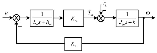
Figure 1. Block diagram of a DC servo motor.

where,

R_a: armature resistance (Ohm); L_a: armature inductance (H)

K_e: back emf constant (V/rad/s); K_m: torque constant (Nm/A)

J_m: inertial moment of the motor shaft (kgm²)

ω: angular velocity of the motor shaft (rad/s)

u: applied voltage to the motor

From Figure 1, the equivalent transfer function of the DC servo motor is obtained as follows:

$$G_M(s)=\frac{\omega (s)}{U(s)}=\frac{K_m}{L_a{J}_m{s}^2+(L_{a}b+R_a{J}_m)s+R_{a}b+K_m{K}_e}$$

(9)

$$G_M(s)=\frac{K_2}{{\tau }_2{s}^2+{\tau }_{1}s+1}$$

(10)

where $K_2=\frac{K_m}{K_m{K}_e+R_{a}b},{\tau }_2=\frac{L_a{J}_m}{K_m{K}_e+R_{a}b},{\tau }_1=\frac{L_{a}b+R_a{J}_m}{K_m{K}_e+R_{a}b}$.

• Case 1: a ball screw system, also called a feed drive system

The block diagram of the mechanical element [6,8] is obtained, as seen in Figure 2:

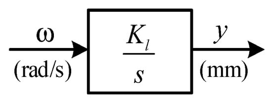
Figure 2. The block diagram of the ball screw.

where ω is the angular velocity (rad/s) of the motor; $K_l=\frac{l}{2\pi }$, and l is the lead of the ball screw (mm); and y is the position of the sliding stable (mm). Therefore, the primary transfer function in this case is obtained:

$$G_l(s)=\frac{K_l}{s}$$

(11)

• Case 2: a rotational mechanism

The block diagram, in this case, can be simplified as Figure 3 [6]:

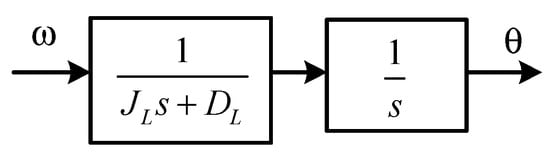
Figure 3. The block diagram of a rotational load.

where $J_L$ is the inertia moment of the rotational load; $D_L$ is viscous damping; and $\theta$ is the rotational angle output (rad). From Figure 3, the transfer function of the primary plant is derived as follows:

$$G_L(s)=\frac{K_L}{s(\tau s+1)}$$

(12)

where $K_L=\frac{1}{D_L}$; $\tau =\frac{J_L}{D_L}$.

3. Analytical Design of FOPI/FOPD Controllers for the Cascade Scheme

3.1. The Control System Structure

The general cascade control system is shown in Figure 4, where $G_{p1}(s)$ and $G_{p2}(s)$ are the transfer functions of the primary and secondary plants, respectively. Additionally, as mentioned above, $G_{p2}(s)$ represents the transfer function of the motor Equation (10) and $G_{p1}(s)$ describes the transfer function of the load in both cases (translational and rotational movement); $G_{c1}(s)$ and $G_{c2}(s)$ are the primary and secondary controllers; and $d_1$ and $d_2$ denote load disturbances affecting each control loop, respectively.

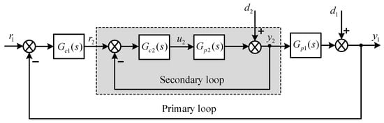
Figure 4. The cascade control system structure.

According to Section 2.4, a dynamic second-order system is used for the secondary model Equation (10).

$$G_{p_2}(s)=G_M(s)=\frac{K_2}{{\tau }_1{s}^2+{\tau }_{2}s+1}$$

(13)

Whereas, for the primary loop, an integrating system or an integrating first-order stable system is adopted as Equation (11) or Equation (12) for both cases of the load, respectively:

$$G_{p_1}(s)=G_l(s)=\frac{K_l}{s}$$

(14)

$$G_{p_1}(s)=G_L(s)=\frac{K_L}{s(\tau s+1)}$$

(15)

3.2. Design of Secondary Controller-Based Direct Synthesis Method

Considering the secondary control loop where its input and output are $r_2$ and $y_2$, respectively, the closed-loop transfer function is obtained:

$$\frac{y_2}{r_2}=\frac{G_{c2}{G}_{p2}}{1+G_{c2}{G}_{p2}}$$

(16)

From Equation (16), the function of the controller is derived as follows:

$$G_{c2}=\frac{1}{{\tilde{G}}_{p2}}\frac{{\left(y_2/r_2\right)}_d}{1-{\left(y_2/r_2\right)}_d}$$

(17)

where ${\tilde{G}}_{p2}$ is the model of the system in the secondary loop, ideally ${\tilde{G}}_{p2}=G_{p2}$; ${\left(y_2/r_2\right)}_d$ represents the desired response of the controlled system. In this paper, a first-order transfer function is chosen for the inner loop; therefore, its transfer function has the following form:

$${\left(\frac{y_2}{r_2}\right)}_d=\frac{1}{{\tau }_{c2}s+1}$$

(18)

where ${\tau }_{c2}$ is the desired time response of the controlled loop and ${\tau }_{c2}$ is chosen to ensure the fastest response with no overshoot of the controlled system.

Replacing (13) and (18) into (17), the general form of $G_{c2}$ is obtained:

$$G_{c2}=\frac{{\tau }_1{s}^2+{\tau }_{2}s+1}{K_2}\frac{1}{{\tau }_{c2}s}$$

(19)

The complex form in frequency domain of the controller is derived by substituting $s=j\omega$ into Equation (19):

$$G_{c2}=\frac{{\tau }_2}{K_2{\tau }_{c2}}-j\frac{1-{\tau }_1{\omega }^2}{K_2{\tau }_{c2}\omega }$$

(20)

Comparing Equations (8) and (20), the control parameters of the secondary control loop are derived:

$$K_{i2}=\frac{{\omega }^{\beta }\left(1-{\tau }_1{\omega }^2\right)}{K_2{\tau }_{c2}\omega \sin {\gamma }_i}$$

(21)

$$K_{p2}=\frac{{\tau }_2}{K_2{\tau }_{c2}}-\frac{{\omega }^{\beta }\left(1-{\tau }_1{\omega }^2\right)\cos {\mathsf{\gamma }}_i}{K_2{\tau }_{c2}{\mathsf{\omega }}^{\beta +1}\sin {\gamma }_i}$$

(22)

3.3. FOPD Controller Design for the Primary Control Loop

The block diagram of the system is reduced in Figure 5 where ${\left(y_2/r_2\right)}_d$ the desired closed-loop transfer function of the inner loop as mentioned above. The closed-loop transfer function of the outer loop (from r₁ to y₁) is described as Equation (23):

$$\frac{Y_1}{R_1}=\frac{G_{c_1}(s){\left(y_2/r_2\right)}_d{G}_{p1}(s)}{1+G_{c_1}(s){\left(y_2/r_2\right)}_d{G}_{p1}(s)}$$

(23)

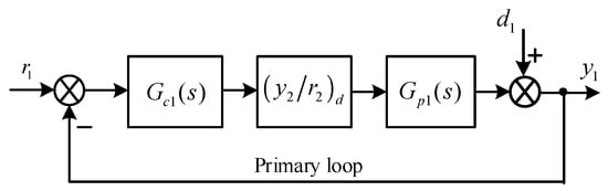
Figure 5. The control structure design of the primary control loop.

• Case 1: The primary plant is a feed drive system, so its transfer function is:   $G_{p1}(s)=\frac{K_l}{s}$

The equivalent of the primary system is considered as the desired transfer function of the inner loop in series with the primary plant. Therefore, the primary transfer function is obtained as follows:

$$G_p(s)={\left(y_2/r_2\right)}_d{G}_{p1}(s)=\frac{1}{{\tau }_{c2}s+1}\frac{K_l}{s}$$

(24)

Similarly to Equation (17), the primary controller is also derived:

$$G_{c1}=\frac{1}{G_p}\frac{\left(y_1/r_1\right)}{1-\left(y_1/r_1\right)}\simeq \frac{1}{{\tilde{G}}_p}\frac{{\left(y_1/r_1\right)}_d}{1-{\left(y_1/r_1\right)}_d}$$

(25)

Ideally, ${\tilde{G}}_p(s)=G_p(s)=\frac{1}{{\tau }_{c2}s+1}\frac{K_l}{s}$; and, in this case,

$${\left(\frac{y_1}{r_1}\right)}_d=\frac{1}{{\tau }_{c1}{s}^{\lambda }+1} (1<\lambda <2)$$

(26)

where $\lambda$ is the fractional order; ${\tau }_{c1}$ is the desired response time of the primary output.

Replacing Equation (26) and ${\tilde{G}}_p$ into Equation (25), the primary controller is obtained:

$$G_{c1}=\frac{s({\tau }_{c2}s+1)}{K_l}\frac{1}{{\tau }_{c1}{s}^{\lambda }}=\frac{({\tau }_{c2}s+1)}{K_l}\frac{1}{{\tau }_{c1}{s}^{{\lambda }_1}}, \mathrm{where} {\lambda }_1=\lambda -1 (0<{\lambda }_1<1)$$

(27)

Substituting $s=j\omega$ to convert $G_{c1}$ into the frequency domain in a complex form:

$$G_{c1}=\frac{{\tau }_{c2}\omega \sin {\gamma }_1+\cos {\gamma }_1}{{\tau }_{c1}{K}_l{\omega }^{{\lambda }_1}}+j\frac{{\tau }_{c2}\omega \cos {\gamma }_1-\sin {\gamma }_1}{{\tau }_{c1}{K}_l{\omega }^{{\lambda }_1}}$$

(28)

Comparing Equations (7) and (28), the control parameters of the primary control loop are obtained:

$$K_{d1}=\frac{{\tau }_{c2}\omega \cos {\gamma }_1-\sin {\gamma }_1}{{\tau }_{c1}{K}_l{\omega }^{{\lambda }_1+\alpha }\sin {\gamma }_d}$$

(29)

$$K_{p1}=\frac{\sin ({\gamma }_1+{\gamma }_d)-{\tau }_{c2}\omega \cos ({\gamma }_1+{\gamma }_d)}{K_l{\tau }_{c1}{\omega }^{{\lambda }_1}\sin {\gamma }_d}$$

(30)

• Case 2: The primary plant is a rotational mechanism,   $G_{p1}(s)=\frac{K_L}{s(\tau s+1)}$

In this case, the equivalent transfer function of the primary plant is:

$$G_p(s)={\left(y_2/r_2\right)}_d G_{p1}(s)=\frac{1}{{\tau }_{c2}s+1}\frac{K_L}{s(\tau s+1)}$$

(31)

Therefore, the primary controller could be calculated as follows:

$$G_{c1}(s)=\frac{1}{G_p}\frac{\left(y_1/r_1\right)}{1-\left(y_1/r_1\right)}=\frac{1}{{\tilde{G}}_p}\frac{{\left(y_1/r_1\right)}_d}{1-{\left(y_1/r_1\right)}_d}$$

(32)

Ideally, ${\tilde{G}}_p(s)=G_p(s)=\frac{1}{{\tau }_{c2}s+1}\frac{K_L}{s(\tau s+1)}$, and ${\left(y_1/r_1\right)}_d$ is chosen as Equation (26) (case 1); therefore, the primary controller is rewritten as follows:

$$G_{c1}(s)=\frac{s({\tau }_{c2}s+1)(\tau s+1)}{K_L}\frac{1}{{\tau }_{c1}{s}^{\lambda }}=\frac{({\tau }_{c2}s+1)(\tau s+1)}{K_L{\tau }_{c1}{s}^{{\lambda }_1}}$$

(33)

where ${\lambda }_1=\lambda -1$ ( $0<{\lambda }_1<1$).

Similarly to case 1, substituting $s=j\omega$ to Equation (33) and rewriting $G_{c1}$ in a complex form:

$$G_{c1}=\frac{(1-\tau {\tau }_{c2}{\omega }^2)\cos {\gamma }_1+\omega (\tau +{\tau }_{c2})\sin {\gamma }_1}{K_L{\tau }_{c1}{\omega }^{{\lambda }_1}}+j\frac{(\tau +{\tau }_{c2})\omega \cos {\gamma }_1-(1-\tau {\tau }_{c2}{\omega }^2)\sin {\gamma }_1}{K_L{\tau }_{c1}{\omega }^{{\lambda }_1}}$$

(34)

Comparing Equations (7) and (34), the control parameters of the primary control loop are obtained in this case:

$$K_{d1}=\frac{(\tau +{\tau }_{c2})\omega \cos {\gamma }_1-(1-\tau {\tau }_{c2}{\omega }^2)\sin {\gamma }_1}{K_L{\tau }_{c1}{\omega }^{{\lambda }_1+\alpha }\sin {\gamma }_d}$$

(35)

$$K_{p1}=\frac{(1-\tau {\tau }_{c2}{\omega }^2)\sin ({\gamma }_1+{\gamma }_d)-(\tau +{\tau }_{c2})\omega \cos ({\gamma }_1+{\gamma }_d)}{K_L{\tau }_{c1}{\omega }^{{\lambda }_1}\sin {\gamma }_d}$$

(36)

3.4. Tuning Procedure Using Maximum Sensitivity Function

From the previous section, it can be seen that the controller parameters are tuned based on some parameters that play an important role in achieving better performance as well as maintaining robustness to model uncertainties. In the proposed method, the maximum sensitivity function is adopted to guarantee the robust stability of each control loop. For a classical feedback control system, the maximum sensitivity function is defined as the following equation:

$$M_s=\underset{\omega }{\max }\left|S(j\omega )\right|$$

(37)

where $S={\left(1+L\right)}^{-1}$, and L is an open-loop transfer function of the system, which normally includes the controller and the system model. Normally, $\left|S\right|$ is small at low frequencies and reaches 1 at high frequencies. However, at some intermediate frequencies, in practice, a peak value of M_s can be larger than 1, which degrades the system performance. Therefore, the peak value of M_s can be used to measure the robustness of the controlled system. In general, for both robust stability and performance, the M_s value should be close to 1. Therefore, in most of the literature, the typical M_s range is chosen from 1.2 to 2 to ensure the robust stability of control systems [36].

For the cascade control scheme in Figure 1, the maximum sensitivity function is suggested for both control loops (inner and outer) as a tuning criterion and its value is assigned as close as possible to 1.2. In this work, this value is used to choose the appropriate frequency to calculate the control parameters of the inner loop ($\omega$ in Equations (21) and (22)), and this frequency is addressed for the outer loop as well. The algorithm to obtain $\omega$ is simple and is described as follows (Algorithm 1):

Algorithm 1: The guideline for tuning parameters based on Ms value

1:  Initialization

$\omega =1$; choose  ${\tau }_{c2}$ and  $\beta$

2:  while  $\left(\omega <1000\right)$ do

3:    Compute  $K_{p2}, K_{i2}$ according to Equations (21) and (22) respectively

4:    Calculate Ms for each set of control parameters

5:     $\omega =\omega +1$

6:  end while

7:  Choose appropriate  $\omega$ to get value of Ms being closed to 1.2

8:  end

4. Robustness Analysis

In this work, the proposed tuning rules are based on the models of actual systems, which are usually represented by nominal models. The differences between the actual system and its model are considered model mismatch or model uncertainty and may degrade some performance indices in terms of servomechanism and regulator problems. Therefore, it is important to analyze the robust stability of model-based methods for control systems in the presence of uncertainties. The multiple sources of parametric and/or unmodelled dynamics uncertainty are commonly grouped into a single lumped perturbation of a specific structure [36].

In this paper, multiplicative output uncertainty is suggested for each control loop of the cascade structure. Therefore, robust stability analysis is carried out herein by considering the multiplicative output uncertainties of each system parameters simultaneously, as shown in Figure 6.

It can be expressed as follows:

$${\Pi }_{O1}: {\overline{G}}_{p1}=(1+E_{O1})G_{p1}; E_{O1}=W_1{\Delta }_1$$

(38)

$${\Pi }_{O2}: {\overline{G}}_{p2}=(1+E_{O2})G_{p2}; E_{O2}=W_2{\Delta }_2$$

(39)

where ${\Pi }_{Oi}$ denotes the set of output perturbed system models; ${\overline{G}}_{pi}$ is the transfer function of the actual model including its nominal model $\left(G_{p1},G_{p2}\right)$ and lumped uncertainty at the output represented by $E_{O1},E_{O2}$. From Equations (38) and (39), ${\Delta }_1,{\Delta }_2$ are normalized perturbation with $\left|{\Delta }_i(j\omega )\right|\le 1, \forall \omega$.

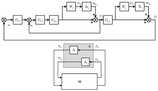
Figure 6. The M-Δ structure using multiplicative output uncertainties of a cascade control system.

According to multiplicative relative uncertainties, the weighting scalar $W_i$ captures the variation of uncertainties over frequencies and has to be chosen to ensure [36]:

$$\left|W_i(j\omega )\right|\ge l_I(\omega )=\underset{{\overline{G}}_{pi}\in {\Pi }_{oi}}{\max }\left|\frac{{\overline{G}}_{pi}(j\omega )-G_{pi}(j\omega )}{G_{pi}(j\omega )}\right|, \forall \omega$$

(40)

To represent unmodelled dynamics, the common simple form of the multiplicative weight is as follows:

$$W_i=\frac{{\tau }_{w}s+r_0}{({\tau }_w/r_{\infty })s+1}$$

(41)

where $r_0$ is the relative uncertainties at low frequencies and $r_{\infty }$ is the magnitude of the weight at high frequencies. It is obvious that $W_i$ is considered as a high-pass filter and, therefore, ${\tau }_w$ is chosen as a cut-off frequency (1/ ${\tau }_w$) to ensure that the weight $W_i$ has a larger magnitude than the largest magnitude of the relative uncertainties in Equation (40).

The structure singular value (denoted SSV, mu, or µ) is suggested to measure the robustness of the control system [36]. In Figure 6, the cascade control scheme with the multiplicative output uncertainty of each loop is rearranged in the M-Δ structure where $\Delta =diag({\Delta }_1,{\Delta }_2)$ and M is a 2 × 2 matrix which includes all remaining blocks such as plants, controllers, and weight factors. To derive M, the relationships between $y_{\Delta }$ and $u_{\Delta }$ are obtained first:

$$\left\{\begin{array}{c}{y}_{{\Delta }_1}=W_1{G}_{p1}{\left(1+G_{p2}{G}_{c2}+G_{p1}{G}_{p2}{G}_{c1}{G}_{c2}\right)}^{-1}\left(u_{{\Delta }_2}-G_{p2}{G}_{c1}{G}_{c2}{u}_{{\Delta }_1}\right)\hfill \\ y_{{\Delta }_2}={\left(1+G_{p2}{G}_{c2}+G_{p1}{G}_{p2}{G}_{c1}{G}_{c2}\right)}^{-1}\left[-G_{c1}{G}_{c2}{G}_{p2}{W}_2{u}_{{\Delta }_1}-\left(G_{p2}{G}_{c2}+G_{p1}{G}_{p2}{G}_{c1}{G}_{c2}\right)W_2{u}_{{\Delta }_2}\right]\hfill \end{array}\right.$$

(42)

Therefore, each element of M can be derived as follows:

$$M_{11}=-W_1{G}_{p1}{G}_{p2}{G}_{c1}{G}_{c2}{\left(1+G_{p2}{G}_{c2}+G_{p1}{G}_{p2}{G}_{c1}{G}_{c2}\right)}^{-1}$$

(43)

$$M_{12}=W_1{G}_{p1}{\left(1+G_{p2}{G}_{c2}+G_{p1}{G}_{p2}{G}_{c1}{G}_{c2}\right)}^{-1}$$

(44)

$$M_{21}=-W_2{G}_{p2}{G}_{c1}{G}_{c2}{\left(1+G_{p2}{G}_{c2}+G_{p1}{G}_{p2}{G}_{c1}{G}_{c2}\right)}^{-1}$$

(45)

$$M_{22}=-W_2{G}_{p2}\left(G_{c2}+G_{c1}{G}_{c2}{G}_{p1}\right){\left(1+G_{p2}{G}_{c2}+G_{p1}{G}_{p2}{G}_{c1}{G}_{c2}\right)}^{-1}$$

(46)

The µ-synthesis states that the control system is stable for all allowed perturbations with $\left|{\Delta }_i(j\omega )\right|\le 1, \forall \omega$ if and only if $\mu \left(M(j\omega )\right)<1, \forall \omega$ [36].

5. Simulation Study

In this paper, the performance indices including the integral absolute error (IAE), the integral time-weighted absolute error (ITAE), and the total variant (TV) are addressed and the smaller values of those indicate better performance. We use the motor and load parameters as seen in Table 1 [38].

Table 1. System parameters.

Symbols	Values	Units
La	8 × 10−5	H
Ra	0.316	Ohm
Jm	1.34 × 10−5	kgm2
b	1.82 × 10−5	Nm/rad/s
Km	0.03	Nm/A
Ke	0.03	V/rad/s
l	0.01	m
JL	6.75 × 10−5	kgm2
DL	1.82 × 10−4	Nm/rad/s

From the parameters in Table 1 and Equation (10), the transfer function of the motor is derived:

$$G_{p2}(s)=\frac{33.1217}{0.00001835s^2+0.0468s+1}$$

(47)

5.1. The Secondary Loop Control Design (Velocity Control)

From Equations (21) and (22), two controller parameters of the inner loop could be obtained. The desired time constant is chosen as ${\tau }_{c2}=0.001$ and the fractional order of the integral term $\beta =1.2$. In this work, to guarantee the robustness of each single loop, the maximum sensitivity function (M_s) is adopted to play a part in tuning control parameters. The proposed algorithm (Section 3.4) is used in this case to obtain values of M_s with respect to $\omega$ as in Figure 7. From the figure, it can be seen that the M_s value converges to 1.2 when increasing $\omega$. However, when $\omega$ is greater than 230 (rad/s), M_s becomes undetermined. Therefore, in this case, we choose $\omega =200$ (M_s = 1.232), and as a result of that, the control parameters are obtained as follows:

$$G_{c2}\left(s\right)=1.426+\frac{24.365}{s^{1.2}}$$

(48)

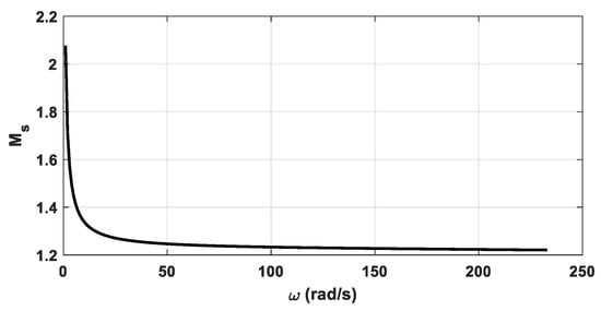
Figure 7. The relationship between maximum sensitivity peak and frequency.

5.2. The Primary Loop Control Design (Position Control)

For the outer loop, in this work, two kinds of plants are considered as mentioned above, a sliding stable or feed drive system and a rotational mechanism. Using the parameters in Table 1, the transfer function of each case is obtained as follows:

$$\mathit{Case} 1: G_{p1}(s)=\frac{0.0016}{s}$$

(49)

In this case, $\alpha =0.6$, ${\tau }_{c1}=0.03$, and from Equation (26), $\lambda =1.1$ is chosen. From Equations (29) and (30), the control parameters are obtained:

$$G_{c1}\left(s\right)=12,196+26.0769s^{0.6}$$

(50)

To justify the effectiveness of the proposed method, the controller settings of both control loops are simulated by providing a ramp function input. In addition, to investigate the effects of disturbances in terms of d₁ for the primary output and d₂ for the secondary output as in Figure 4, two step changes of these are inserted at times t = 1 (s) and t = 5 (s), respectively. Figure 8 and Figure 9 illustrate the closed-loop responses at the primary output (position) and secondary output (velocity) in this case. From the figures, it can be seen that the tracking control completely meets the servo performance requirements (fast response and no overshoot or oscillation). The disturbance of the secondary loop (d₂) does not have any effect on the primary output. In contrast, at time t = 5, there is a variation in position due to d₁; however, the primary controller maintains the performance in an excellent way. The control signals are shown in Figure 10 to prove that the proposed method has smooth control signals, which is the disadvantage of some advanced control techniques.

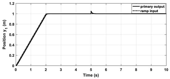
Figure 8. The translation responses to the ramp input with disturbances.

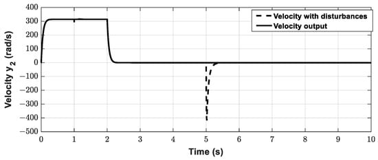
Figure 9. The velocity responses of case 1 with and without disturbances.

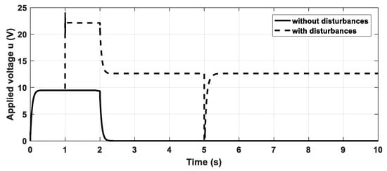
Figure 10. The applied voltages in both cases.

Moreover, the robustness of the proposed controller will be shown, as mentioned in Section 4. To obtain $l_I(\omega )$ in Equation (40), the nominal parameters of the inner transfer function are changed in the range of ±50%. The corresponding relative errors $\left|({\overline{G}}_{p_1}-G_{p_1})/G_{p_1}\right|$ are shown as functions of frequency in Figure 11a, and it can be seen that $l_I(\omega )$ is 0.4 at low frequencies and 5 at high frequencies. ${\tau }_w$ is chosen to guarantee that $W_2$ is large enough to satisfy $W_2>l_I(\omega )$ at all frequencies. From the figure, ${\tau }_w=0.0667$; therefore, the transfer function of $W_2$ is obtained (from Equation (41)). For the outer loop (Figure 11b), it can be performed similarly, finally also obtaining the transfer function of $W_1$ in this case with ${\tau }_w=0.01, r_0=0.4,$ and $r_{\infty }=1.5$.

$$W_1=\frac{0.01s+0.4}{(0.01/1.5)s+1}$$

(51)

$$W_2=\frac{0.0667s+0.4}{(0.0667/5)s+1}$$

(52)

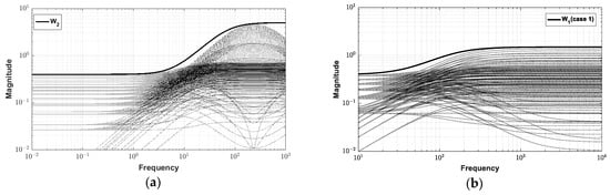
Figure 11. (a,b) The scalar multiplicative weights of both control loops.

Figure 12 illustrates the structured singular value (SSV) of the M-Δ structure using From Equations (43)–(46), when two sources of parametric uncertainties of both control loops affect simultaneously, two scalar weight transfer functions W₁ and W₂ are as above. As mentioned in Section 4, the condition for robust stability is that the µ value has to be always less than 1. From the figure, it is obvious that the peak of µ is 0.4 over the frequency range, which ensures the robustness of the controlled system.

$$\mathit{Case} 2: G_{p1}(s)=\frac{2}{s(0.0014s+1)}$$

(53)

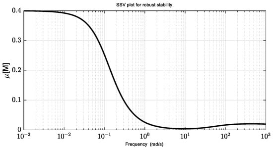
Figure 12. The SSV plot for robust stability of case 1.

In this case, $\alpha =0.9$, ${\tau }_{c1}=0.02$, and from Equation (26), $\lambda =1.2$ is chosen. From Equations (35) and (36), the control parameters are obtained:

$$G_{c1}\left(s\right)=8.8414+0.0115s^{0.9}$$

(54)

In this case, the position output is the rotational angle (rad), and the ramp function input is adopted to verify the position control problem. Two disturbances described in Figure 4 are illustrated by adding step signals at time t = 1 (s) and t = 5 (s). Figure 13 and Figure 14 show the closed-loop responses at the primary output (position) and secondary output (velocity) in two cases. From the figure, it can be seen that the tracking control completely satisfies the servo performance requirements (fast response and no overshoot or oscillation). The disturbance in the inner loop has no effect on the primary output. This means that the effectiveness of the cascade scheme is clarified in this case. The primary controller plays an important part in maintaining the position in a servo manner. The control signals are shown in Figure 15. It can be seen that, in this case, the proposed method also has a smooth control signal, and only are there sudden changes in the manipulated variable due to the disturbances.

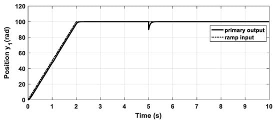
Figure 13. The rotational responses to the ramp input with disturbances.

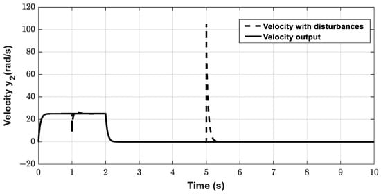
Figure 14. The velocity responses of case 2 with and without disturbances.

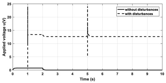
Figure 15. Applied voltages for both cases.

This is similar to case 1, to obtain $l_I(\omega )$ in Equation (40), the nominal parameters of the inner transfer function are changed in the range of ±50%, approximately. Figure 16 illustrates the relative errors and it can be seen that $l_I(\omega )$ is 0.5 at low frequencies and 1.1 at high frequencies. ${\tau }_w$ is chosen as 0.002 to satisfy $W_1>l_I(\omega )$ at all frequencies. Therefore, the transfer function of $W_1$ is as Equation (55). Note that the transfer function of $W_2$ is still the same as the one in case 1.

$$W_1=\frac{0.002s+0.5}{(0.002/1.1)s+1}$$

(55)

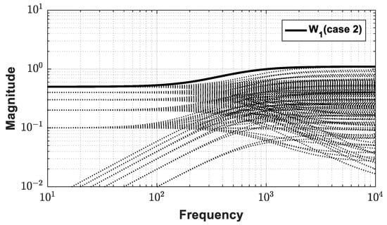
Figure 16. The scalar multiplicative weight of the primary loop of case 2.

Figure 17 illustrates the SSV plot of the M-Δ structure in this case. From the figure, it can be seen that the peak of µ is 0.52 over the frequency range, which ensures the robustness of the controlled system.

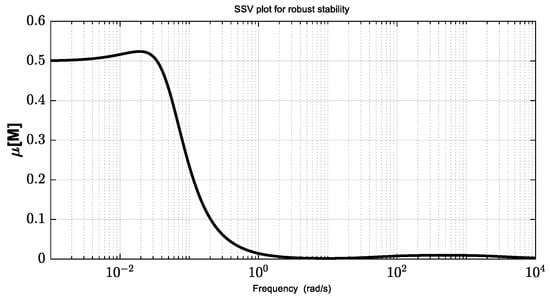
Figure 17. The SSV plot for robust stability of case 2.

The robust performance of the controlled systems is also evaluated by perturbing ±20% to all plant parameters. The performance indices are tabulated in Table 2 of nominal models and perturbed ones. From the data, it is obvious that the controlled systems still keep good tracking control in the presence of uncertainties, and the µ values are practically the same as the ones of the nominal models.

Table 2. The performance indices in nominal and perturbed models for both cases.

	Case 1				Case 2
	IAE	ITAE	TV	µ (M)	IAE	ITAE	TV	µ (M)
Nominal	0.0515	0.0543	21.06	0.40	5.655	5.971	1.949	0.524
Perturbed (±20%)	0.0962	0.3693	18.63	0.42	8.801	29.883	1.543	0.5243

6. Conclusions

The fractional-order control designs for servo systems are studied in this work. To achieve the strict requirements of control performance in terms of fast response and no overshot/oscillation, the cascade control structure including two control loops, the secondary loop (inner loop) for velocity control and the primary loop (outer loop) for position control, is proposed. The FOPI and FOPD are suggested for the inner and outer, respectively, and the analytical design methods in the frequency domain are also proposed to derive the tuning rules for both controllers. In the inner loop, the maximum sensitivity function is adopted to choose the appropriate frequency to ensure the robustness of this control loop. The M-Δ structure is also addressed to justify the robustness of the controlled system using multiplicative output uncertainties, for which parametric uncertainties of both control loops are considered simultaneously. The simulation results indicate that the proposed method consistently satisfies the system requirements with a fast and no overshoot closed-loop time response to ramp function inputs. The performance indexes also clarify the effectiveness of the proposed method. The robust stability is also verified by the µ value, which has a peak value of less than 1 over the frequency range in all cases.

References

- Lim, H.; Seo, J.W.; Choi, C.H. Position control of XY table in CNC machining center with non-rigid ball screw. In Proceedings of the 2000 American Control Conference, ACC (IEEE Cat. No. 00CH36334), Chicago, IL, USA, 28–30 June 2000; Volume 3. [Google Scholar]
- Franks, R.G.; Worley, C.W. Quantitative analysis of cascade control. Ind. Eng. Chem. 1956, 48, 1074–1079. [Google Scholar] [CrossRef]
- Chen, J.S.; Huang, Y.; Cheng, K. Mechanical model and contouring analysis of high-speed ball-screw drive systems with compliance effect. Int. J. Adv. Manuf. Technol. 2004, 24, 241–250. [Google Scholar] [CrossRef]
- Altintas, Y.; Verl, A.; Brecher, C.; Uriarte, L.; Pritschow, G. Machine feed drives. CIRP Ann. Manuf. Technol. 2011, 60, 779–796. [Google Scholar] [CrossRef]
- Hwan, S.S.; Kang, S.K.; Chung, D.H.; Stroud, I. Theory and Design of CNC Systems; Springer: Cham, Switzerland, 2008; pp. 157–185. [Google Scholar]
- Nakamura, M.; Goto, S.; Kyura, N. Mechatronic Servo System Control; Springer: Cham, Switzerland, 2004. [Google Scholar]
- Sato, R.; Tsutsumi, M. Mathematical model of feed drive systems consisting of AC servo motor and linear ball guide. J. Jpn. Soc. Precis. Eng. 2005, 71, 633–638. [Google Scholar] [CrossRef]
- Sato, R.; Tsutsumi, M. Modeling and controller tuning techniques for feed drive systems. In Proceedings of the ASME 2005 International Mechanical Engineering Congress and Exposition, Orlando, FL, USA, 5–11 November 2005; pp. 669–679. [Google Scholar]
- Liu, Y.; Wang, Z.Z.; Wang, Y.F.; Wang, D.H.; Xu, J.F. Cascade tracking control of servo motor with robust adaptive fuzzy compensation. Inf. Sci. 2021, 569, 450–468. [Google Scholar] [CrossRef]
- Lee, Y.; Park, S.; Lee, M. PID controller tuning to obtain desired closed loop responses for cascade control systems. Ind. Eng. Chem. Res. 1998, 37, 1859–1865. [Google Scholar] [CrossRef]
- Rao, A.S.; Seethaladevi, S.; Uma, S.; Chidambaram, M. Enhancing the performance of parallel cascade control using Smith predictor. ISA Trans. 2009, 48, 220–227. [Google Scholar] [PubMed]
- Uma, S.; Chidambaram, M.; Rao, A.S.; Yoo, C.K. Enhanced control of integrating cascade processes with time delays using modified Smith predictor. Chem. Eng. Sci. 2010, 65, 1065–1075. [Google Scholar] [CrossRef]
- Padhan, D.G.; Majhi, S. An improved parallel cascade control structure for processes with time delay. J. Process Control 2012, 22, 884–898. [Google Scholar] [CrossRef]
- Santosh, S.; Chidambaram, M. A simple method of tuning parallel cascade controllers for unstable FOPTD systems. ISA Trans. 2016, 65, 475–486. [Google Scholar] [CrossRef]
- Raja, G.L.; Ali, A. Modified parallel cascade control strategy for stable, unstable and integrating processes. ISA Trans. 2016, 65, 394–406. [Google Scholar] [CrossRef] [PubMed]
- Raja, G.L.; Ali, A. Smith predictor based parallel cascade control strategy for unstable and integrating processes with large time delay. J. Process Control 2017, 52, 57–65. [Google Scholar] [CrossRef]
- Neubauer, M.; Brenner, F.; Hinze, C.; Verl, A. Cascaded sliding mode position control (SMC-PI) for an improved dynamic behavior of elastic feed drives. Int. J. Mach. Tools Manuf. 2021, 169, 103796. [Google Scholar] [CrossRef]
- Sun, G.; Wu, L.; Kuang, Z.; Ma, Z.; Liu, J. Practical tracking control of linear motor via fractional-order sliding mode. Automatica 2018, 94, 221–235. [Google Scholar] [CrossRef]
- Wang, J.; Shao, C.; Chen, Y.Q. Fractional order sliding mode control via disturbance observer for a class of fractional order systems with mismatched disturbance. Mechatronics 2018, 53, 8–19. [Google Scholar] [CrossRef]
- Wang, S.; Yu, H.; Yu, J. Robust adaptive tracking control for servo mechanisms with continuous friction compensation. Control Eng. Pract. 2019, 87, 76–82. [Google Scholar] [CrossRef]
- Xu, H.; Hinze, C.; Lechler, A.; Verl, A. Robust µ parameterization with low tuning complexity of cascaded control for feed drives. Control Eng. Pract. 2023, 138, 105607. [Google Scholar] [CrossRef]
- Zou, M.; Yu, J.; Ma, Y.; Zhao, L.; Lin, C. Command filtering-based adaptive fuzzy control for permanent magnet synchronous motors with full-state constraints. Inf. Sci. 2020, 546, 1–12. [Google Scholar] [CrossRef]
- Nassef, A.M.; Abdelkareem, M.A.; Maghrabie, H.M.; Baroutaji, A. Metaheuristic-based algorithms for optimizing fractional-order controllers—A recent, systematic, and comprehensive preview. Fractal Fract. 2023, 7, 553. [Google Scholar] [CrossRef]
- Podlubny, I. Fractional-Order Systems and PIλDμ-Controllers. IEEE Trans. Autom. Control 1999, 44, 208–214. [Google Scholar] [CrossRef]
- Padula, F.; Visioli, A. Tuning rules for optimal PID and fractional-order PID controllers. J. Process Control 2011, 21, 69–81. [Google Scholar] [CrossRef]
- Vu, T.N.L.; Lee, M. Analytical design of fractional-order proportional-integral controllers for time-delay processes. ISA Trans. 2013, 52, 583–591. [Google Scholar] [CrossRef] [PubMed]
- Beschi, M.; Padula, F.; Visioli, A. Fractional robust PID control of a solar furnace. Control Eng. Pract. 2016, 56, 190–199. [Google Scholar] [CrossRef]
- Li, D.; Liu, L.; Jin, Q.; Hirasawa, K. Maximum sensitivity based fractional IMC-PID controller design for non-integer order system with time delay. J. Process Control 2015, 31, 17–29. [Google Scholar] [CrossRef]
- Vilanova, R.; Arrieta, O.; Ponsa, P. Robust PI/PID controllers for load disturbance based on direct synthesis. ISA Trans. 2018, 81, 177–196. [Google Scholar] [CrossRef] [PubMed]
- Yumuk, E.; Guzelkaya, M.; Eksin, I. Analytical fractional PID controller design based on Bode’s ideal transfer function plus time delay. ISA Trans. 2019, 91, 196–206. [Google Scholar] [CrossRef]
- Moradi, M. A genetic-multivariable fractional order PID control to multi-input multi-output processes. J. Process Control 2014, 24, 336–343. [Google Scholar] [CrossRef]
- Sánchez, H.S.; Padula, F.; Visioli, A.; Vilanova, R. Tuning rules for robust FOPID controllers based on multi-objective optimization with FOPDT models. ISA Trans. 2017, 66, 334–361. [Google Scholar] [CrossRef] [PubMed]
- Tumari, M.Z.M.; Ahmad, M.A.; Suid, M.H.; Hao, M.R. An improved marine predators algorithm-tuned fractional-order PID controller for automatic voltage regulator systems. Fractal Fract. 2023, 7, 571. [Google Scholar] [CrossRef]
- Shalaby, R.; El-Hossainy, M.; Abo-Zalam, B.; Mahmoud, T.A. Optimal fractional-order PID controller based on fractional-order actor-critic algorithm. Neural Comput. Appl. 2022, 35, 2347–2380. [Google Scholar] [CrossRef]
- Vu, T.N.L.; Chuong, V.L.; Truong, N.T.N.; Jung, J.H. Analytical Design of Fractional-Order PI Controller for Parallel Cascade Control Systems. Appl. Sci. 2022, 12, 2222. [Google Scholar] [CrossRef]
- Skogestad, S.; Postlethwaithe, I. Multivariable Feedback Control Analysis and Design, 2nd ed.; John Wiley & Sons: Hoboken, NJ, USA, 2001; pp. 253–351. [Google Scholar]
- Monje, C.A.; Chen, Y.; Vinagre, B.M.; Xue, D.; Feliu-Batlle, V. Fractional-Order Systems and Controls, Fundamentals and Applications; Springer: London, UK, 2010. [Google Scholar]
- Choudhary, K.; Qureshi, M.S.; Singh, B. Position Control of DC Motor using Improved Sliding Mode Control Techniques. Int. J. Appl. Eng. Res. 2018, 13, 15–19. [Google Scholar]
Disclaimer/Publisher’s Note: The statements, opinions and data contained in all publications are solely those of the individual author(s) and contributor(s) and not of MDPI and/or the editor(s). MDPI and/or the editor(s) disclaim responsibility for any injury to people or property resulting from any ideas, methods, instructions or products referred to in the content. |
© 2024 by the authors. Licensee MDPI, Basel, Switzerland. This article is an open access article distributed under the terms and conditions of the Creative Commons Attribution (CC BY) license (https://creativecommons.org/licenses/by/4.0/).