Statistical Study of the Bias and Precision for Six Estimation Methods for the Fractal Dimension of Randomly Rough Surfaces

Abstract

The simulation and characterisation of randomly rough surfaces is an important topic in surface science, tribology, geo- and planetary sciences, image analysis and optics. Extensions to general random processes with two continuous variables are straightforward. Several surface generation algorithms are available, and preference for one or another method often depends on the specific scientific field. The same holds for the methods to estimate the fractal dimension D. This work analyses six algorithms for the determination of D as a function of the size of the domain, variance, and the input value for D, using surfaces generated by Fourier filtering techniques and the random midpoint displacement algorithm. Several of the methods to determine fractal dimension are needlessly complex and severely biased, whereas simple and computationally efficient methods produce better results. A fine-tuned analysis of the power spectral density is very precise and shows how the different surface generation algorithms deviate from ideal fractal behaviour. For large datasets defined on equidistant two-dimensional grids, it is clearly the most sensitive and precise method to determine fractal dimension.

1. Introduction

The description of surface topography by the superposition of harmonic waves with randomly oriented wave vectors and phase angles was pioneered by Longuet-Higgins in relation to the moving sea surface [1,2]. It uses the relationship between the magnitude of the wave vector and the power spectrum (PS). Whitehouse et al. [3] were among the first to analyse the roughness of engineering surfaces under the concept of random process theory. With increasing measurement size and resolution, it was found that roughness increases with the length (area) of the measured domain [4,5,6,7].

Fractals are often associated with graphics in a plane, such as the Julia and Mandelbrot sets [8] or with problems like the coastline paradox [9], explained in terms of a Hausdorff dimension in a classical paper by Mandelbrot [10]. A geometrical analysis of fractal dimension follows naturally from the graphical nature of the object studied. For random fractal surfaces, or more generally, for the self-affine stochastic processes found in many scientific disciplines, the problem must be approached differently. A mathematical definition of the basic problem is the most direct way to start.

The increase in the variance with an increase in the size of the domain over which the random variable is measured follows from Plancherel’s theorem [11] for self-affine surfaces with a power-law PS: let the surface topography be described as a function $z\left(x,y\right)$, with an isotropic PS:

$$P\left(r\right)=\{\begin{array}{cc}0& r<r_l\\ C{r}^{-2\left(H+1\right)}& r_l<r<r_u\\ 0& r_u\end{array}$$

(1)

Here, $r=\sqrt{k^2+l^2}$, the magnitude of the wave vector k with components $\left(k,l\right)$. $r_l$ and $r_u$ are the lower and upper cut-off radii in the frequency domain. C is a constant. The measurement length corresponds to the maximum wavelength ${\lambda }_u=2\mathsf{\pi }/r_l$ and the resolution of the measurement ${\lambda }_l=2\mathsf{\pi }/r_u$, where H is the Hurst exponent and the fractal dimension $D=3-H$. The variance of the height is given by the following:

$$z^2={{\displaystyle \int }}_0^{\infty }2\mathsf{\pi }rP\left(r\right)dr=\mathsf{\pi }C\frac{r_l^{-2H}-r_u^{-2H}}{H}$$

(2)

The operator $<·>$ refers to the expected value. For $r_l/r_u\ll 1$, the second term in the numerator can be neglected, and the standard deviation $\sigma =\sqrt{z^2}~r_l^{-h}~{\lambda }_u^h$, i.e., the root mean square roughness increases with the measurement length ${\lambda }_u$.

It has been shown that ${\lambda }_l$ can be of atomic size in diamond coatings [12,13], while ${\lambda }_u$ can be as large as the size of the observable universe [14]. The cut-off radii are generally not imposed by the physics of the phenomenon but by instrumental limitations, although a combination of measurement techniques at overlapping observation scales has been used to successfully extend ${\lambda }_u/{\lambda }_l$ [4,12,13]. In geo- and planetary sciences, multifractal descriptions are often used, where the value of H is allowed to vary with ${\lambda }_u$ and/or ${\lambda }_l$ [15,16,17]. In materials science and tribology, an upper cut-off ${\lambda }_u$ is universally observed, beyond which the roughness no longer increases with the measurement length [12,13,18]. ${\lambda }_u$ can be associated with the intuitive concept of coarseness, while H can be connected to complexity [19]. In numerical simulations, ${\lambda }_u/{\lambda }_l$ is determined by the size of the dataset, and ${\lambda }_u$ can be set to 1 without loss of generality.

Different definitions of the fractal dimension can give different results for D [20]. A distinction must be made between the mathematical definition of D and the numerical methods used to estimate D from a discrete set of measured or simulated data. From a mathematical viewpoint, it is sufficient to find a single example in which two definitions of D produce different results. Although there are many counterexamples, the Minkowski and Hausdorff dimensions coincide in almost all cases, and objective criteria exist to test this coincidence [21].

In numerical methods, if $D_{\mathcal{M}}$ is the estimate of D by a given method $\mathcal{M}.$ If two methods produce distinct values $D_{\mathcal{M}}$, it must be checked if they correspond to established mathematical exceptions. If not, the difference is more likely due to the numerical procedure missing some essential details of the geometry or because of the finite size and resolution of the available dataset. All definitions of fractal dimensions involve a limit for ${\lambda }_l\to 0$. Limitations on ${\lambda }_u/{\lambda }_l$ may severely distort the relationship between $D_{\mathcal{M}}$ and $D$.

Most methods for determining D are only applicable to a limited subset of geometries [20]. This study assumes that a smooth reference surface exists on a simply connected domain on which a function $z\left(x,y\right)$ can be defined. For engineering surfaces and many geological and geomorphological studies, z is the height. More generally, z can be any random variable measured along a line or surface, such as the grey scale or colour value of pixels in an image [22,23,24,25] or the temperature of the cosmic background radiation [26,27]. Contours of constant $z_0=z\left(x,y\right)$ (or $w_0=w\left(x,y,z\right)$ in three dimensions [28]) cannot be analysed by the methods studied here, except for box counting methods (BCM) and a strongly modified power spectral density method [29].

This work will provide clear definitions of the bias and precision of the different methods $\mathcal{M}$ for the determination of H, with the goal of determining which method provides the best estimate for H. Section 2 of this paper describes the methods used to simulate the random surfaces and calculate H. Section 2.1 explains how this combination defines a random process. Section 2.2 presents three surface generation algorithms. It justifies the selection of only two of them for further analysis. The following seven subsections describe the methods used for determining H. Section 3 describes the simulation scheme, identifies the parameters of interest, and provides a statistical analysis of the results based on linear regression and analysis of variance (ANOVA). The results are discussed in terms of bias, dispersion, precision, and computational and information efficiency. This will allow us to reach a clear conclusion with respect to the problem posed in the title of this paper.

2. Methods

2.1. Surface Simulation and Characterisation as a Random Process

Simulated surfaces will be used to analyse the methods for estimating H. The process is illustrated in Figure 1. For Gaussian surfaces with zero mean, the input values are the variance $<z^2{>}_{in}$, $H_{in}$, ${\lambda }_u$, and ${\lambda }_l$. These are deterministic values. The surface generation algorithm $\mathcal{S}$ acts on a finite set $\left\{g_i\right\}$ of random values, producing a single representation $z_{\mathcal{S}}\left(x,y\right)$. Because of the random nature of $\left\{g_i\right\}$, the mean value of ${\mu }_{\mathcal{S}}\ne 0$ and $<z^2{>}_{\mathcal{S}}\ne <z^2{>}_{in}$ in general. Shifting and rescaling the simulated surface can correct these random variations. A numerical procedure $\mathcal{M}$ then calculates the simulated Hurst exponent $H_{\mathcal{S}\mathcal{M}}$ (or $H_{out}$), which is a random variable, which will be characterised by its mean and standard deviation.

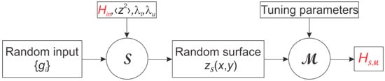
Figure 1. Representation of the process which creates $H_{\mathcal{S}\mathcal{M}}$ for a given input value $H_{in}$ through a surface generating algorithm $\mathcal{S}$ and a method $\mathcal{M}$. By the random input $\left\{g_i\right\}$, $z_{\mathcal{S}}\left(x,y\right)$ is a random process, and $H_{\mathcal{S}\mathcal{M}}$ is a random value.

The bias is defined as $B_{\mathcal{S}\mathcal{M}}\left(H_{in}\right)=<H_{\mathcal{S}\mathcal{M}}>-H_{in}$. The variance $<H_{\mathcal{S}\mathcal{M}}^2>\ne <H_{\mathcal{S}}^2>$; the right-hand side is the variance of the unknown Hurst exponent of the surface simulated with $\mathcal{S}$. The total dispersion can be characterised by the standard deviation ${\sigma }_{out}\left(H_{in}\right)=\sqrt{<{\left(H_{\mathcal{S}\mathcal{M}}-H_{in}\right)}^2>}$. $<H_{\mathcal{S}}^2>$ cannot be estimated independently of $\mathcal{M}$, but the smallest $<H_{\mathcal{S}\mathcal{M}}^2>$ obtained from a given set of methods will give an upper bound estimate for $<H_{\mathcal{S}}^2>$.

2.2. Surface Generation

Surfaces used in this study are defined on an equidistant set of points $\left(x_i,y_j\right)$, with $i,j:1\to 2^{n_0}$ and $n_0$ = 8, 9, or 10. The side of the square domain can be arbitrarily set equal to 1. Then, ${\lambda }_u=\sqrt{2}$ and ${\lambda }_l=2^{-n_0}$. Three surface generation methods $\mathcal{S}$ are commonly used to generate $z\left(x,y\right)$. The generalised Weierstrass–Mandelbrot function [30,31] ($\mathcal{S}=WM$) has recently recovered some popularity [32,33,34,35,36,37,38]. It is described by the following:

$$z\left(x,y\right)={\lambda }_u{\left(\frac{G}{{\lambda }_u}\right)}^{D-2}\sqrt{\frac{\log \gamma }{M}}{\sum }_{m=1}^M{\sum }_{n=0}^N{\gamma }^{\left(D-3\right)n}\cos \left({\phi }_{nm}-\cos \left(2\mathsf{\pi }{\gamma }^n\sqrt{x^2+y^2}\cos \left(\arctan \left(\frac{x^2}{y^2}\right)-\frac{\mathsf{\pi } m}{M}\right)+{\phi }_{nm}\right)\right).$$

(3)

G is called the fractal roughness, and $\gamma$ is the lacunarity. The random phase angles ${\phi }_{mn}$ are chosen from a uniform distribution on $\left[-\mathsf{\pi },\mathsf{\pi }\right]$. The observation that the second cosine term in the sum is independent from the random phase angles allows speeding up the calculation of the WM surface during Monte Carlo simulations. Even so, the method is not computationally efficient compared to the following algorithms.

The midpoint displacement method ($\mathcal{S}=MP$) has been widely used in computer graphics [39] and in early studies on fractal landscapes [40,41]. The original midpoint algorithm suffers from the problem that the initial few values can dominate the entire simulated surface, creating clear cross-patterns in the result. This can be corrected by modifying the way in which random values are added during each simulation step [39]. It is also feasible to ensure periodicity of the surface, which is important in some simulations, e.g., in contact mechanics, where a Fourier transform boundary element method is employed [42,43].

The Fourier transform method ($\mathcal{S}=FT$) [43,44] uses normally distributed variables $\left\{g_{ij}\right\}$ on a regular grid with a size of $2^{n_0}\times 2^{n_0}$. This set is transformed to the frequency domain using a fast Fourier transform (FFT), defining $\left\{\widehat{g_{ij}}\right\}=\mathcal{F}\left\{g_{ij}\right\}$. By multiplying with the PS $P\left(k,l\right)$ in the frequency domain and applying the inverse Fourier transform (IFT), $\left\{\widehat{g_{ij}}\right\}$is filtered:

$$z\left(x,y\right)={\mathcal{F}}^{-1}\left(\left(Re\left(\widehat{g_{ij}}\right)+\mathrm{i} Im\left(\widehat{g_{ij}}\right)\right)\sqrt{P\left(\sqrt{k_i^2+l_i^2}\right)}\right),$$

(4)

where $\mathrm{i}=\sqrt{-1}$; the linear combination of real and imaginary parts in Equation (4) generates a purely real $z\left(x,y\right).$

It shall be remembered that the FFT is only an efficient way of summing cosine and sine terms in a discrete Fourier transform (DFT). This is equivalent to the original approach by Longuet-Higgins [1], but Equation (4) allows for the efficient inclusion of $2^{2n_0}$ harmonic terms, which would require unacceptable computer times if the surface were generated by naive algorithms. However, by using the FFT, aliasing is introduced, which results in a statistical height distribution that is not Gaussian. This aspect can be improved by eliminating the longest wavelengths from the analysis [45].

Figure 2 shows three topographies generated by WM, MP, and FT. Their differences are seen in $P_{\mathcal{S}}$ and the autocorrelation $R_{\mathcal{S}}$ (Section 2.7). $P_{WM}$ shows many individual peaks corresponding to the individual combinations $\left(m,n\right)$ in Equation (3) and has ridges along the coordinate axes. The rotational symmetry inherent to Equation (3) is visible in $R_{WM}$ as small wrinkles in the conical part of the surface. Elaborating Equation (3) is computationally inefficient and limits the use of WM for large-scale simulations.

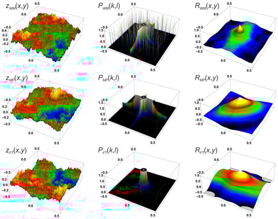
Figure 2. Height maps $z_{\mathcal{S}}\left(x,y\right)$, power spectra $P_{\mathcal{S}}\left(k,l\right)$, and autocorrelation $R_{\mathcal{S}}\left(x,y\right)$ (see Section 2.5) for $\mathcal{S}=WM$ (N = 18, M = 23), $\mathcal{S}=MP,$ and $\mathcal{S}=FT$; $n_0=10$.

$P_{MP}$ and $R_{MP}$ show pronounced edges along the coordinate axes. The preferential 90°–45° orientations imposed by the algorithm are clearly visible in $R_{MP}$. $P_{FT}$ consists of a noisy signal around the centre of the spectrum that decays according to Equation (1). $R_{FT}$ consists of a conical peak superposed on a background ridge. Only the conical part is important for the analysis (Section 2.8).

2.3. Box Counting Methods

Box counting methods (BCM) are, in principle, numerical implementations of the theoretical definition of a Minkowski dimension [18]. For fractal curves defined on a unit square domain, the method consists of dividing the image into a set of $m\times m$ identical squares with length a = 1/m and counting the number n_m of squares which contain at least one point of the curve. The box counting dimension is determined as the following:

$$D_{BCM}=\underset{m\to \infty }{\lim }\frac{\log n_m}{\log m}$$

(5)

If there is an algorithm for infinitely refining the scale of the curve, m is limited only by computational precision, and the method is very accurate [46,47,48]. For experimental data, m is limited by the spatial resolution. The procedure is analogous in 3 dimensions [28].

For functions defined as $z\left(x,y\right)$ on a finite grid, the method produces considerable bias [49]. Several recent publications have focussed on the rule that n_m should be the infimum of all possible covering configurations at a given size [22,50]. This infimum can be approximated by shifting the covering boxes with respect to their ideal position [51]. Differential box counting (DBC) adapts for differences in vertical and horizontal scale by calculating the range $∆z$ over the domain and using boxes of vertical size $∆z/m$. A lack of vertical resolution is addressed by considering only the highest and lowest boxes that contain part of the surface in each column of boxes; all intermediate boxes will contain a part of the surface, even if the corresponding points do not appear in the dataset [49]. This modifies Equation (5) as the following:

$$D_{DBC}=\underset{m\to \infty }{\lim }\frac{\log {\sum }_i\lceil m\frac{M_i-m_i}{∆z}\rceil }{\log m}$$

(6)

where the sum is taken over all $m^2$ boxes, $\lceil ·\rceil$ represents the ceiling function, and $M_i$ and $m_i$ are the maximum and minimum values within square i. The method is closely related to the Hall–Wood estimator [52,53]. Differences between the original definition of a box counting dimension, BCM and DBC, are illustrated in Figure 3.

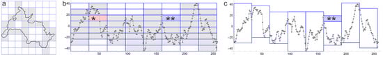
Figure 3. (a) Original concept of BCM as a method to estimate the Minkowski dimension of a fractal contour. The grey boxes contain part of the curve and are counted in $n_m$. (b) BCM with vertical scaling. The boxes marked by * and ** are missed because the curve passes through the box, but there are no data points inside the box due to a lack of vertical resolution. (c) DBC allows for a vertical shift and counts the total range in individual intervals. Box ** is still missed.

Notice that Figure 3, Figure 4 and Figure 5 use time series to exemplify the basic concepts of the methods and are for illustrative purposes only. The curve shown in Figure 3a and Figure 4a corresponds to an arbitrary contour line of a surface produced by FT. The data series represents an arbitrary vertical section through this surface in arbitrary units. All methods described in this paper refer to the fully three-dimensional functions, as shown in Figure 2.

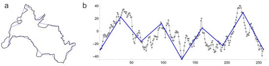
Figure 4. (a) Original concept of the yardstick method to estimate the Hausdorff dimension of a fractal contour. The contour is approximated by lines of a fixed length. (b) Trapezium method [39] for the estimation of the fractal dimension of a time series. The length of the lines between the dots is approximated by the length of the blue lines over intervals of width a in successive refinements. By Pythagoras’ theorem, the method is sensitive to vertical scaling, and the finite resolution of the data means that the limit for $a\to 0$ can only be approached crudely.

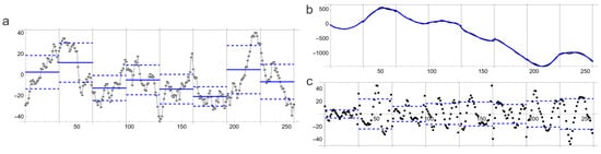
Figure 5. (a) Illustration of RLM for a time series. The vertical variation (standard deviation) is marked as dashed lines relative to the mean (blue line). (b) Cumulative data (black) with superposed piecewise fitting curves (blue, Equation (9)), according to DBC. (c) Fitting residuals, showing the residual standard deviation (dashed line) for each interval. Standard deviations are shown for plotting purposes; RLM and DBC use the corresponding variance.

2.4. Triangular Prism Method

The triangular prism method (TPM) [40,41,54] is an extension of the Hausdorff dimension as used by Mandelbrot [10] to explain the coastline paradox [9]. The original method is applied to contour lines in the plane, where the number $n_i$ of segments (yardsticks) with a given length $l$ required to cover the entire contour is determined by geometrical construction. TPM extends this approach by covering a surface with a mesh of triangles of a given size. The total surface area $s_{Tot}$ is the sum of all areas obtained by approximating the surface by triangles over a grid of square domains with side a and the following equation:

$$D_{TPM}=\underset{a\to 0}{\lim }\frac{\log s_{Tot}}{\log a}$$

(7)

Because surface area does not linearly scale with height, this method is sensitive to the vertical scale, which would limit its use to self-similar surfaces [55]. However, it has been proven that Equation (7) always converges to the correct value of D, but very small values of a may be required, corresponding to very large datasets [46]. The difference between the original definition of a Hausdorff dimension and its application to a time series is shown in Figure 4. For more details on the geometry in the case of two-dimensional surfaces, the reader is referred to Ref. [49].

2.5. Detrended Fluctuation

Detrended fluctuation (DTF) was originally developed for the study of single-variable processes that show nonstationarity [56]. Instead of analysing the variance of the function over a time interval $∆t$, a linear or polynomial fit is made to the accumulated function over $∆t$, and the residual variance of this fit is analysed as a function of $∆t$. The method was adapted to two-variable random processes by Gu and Zhou [57,58], with an emphasis on multifractal analysis.

Here, the cumulative function $Z\left(x,y\right)$ is calculated over each square subdivision with side a. A fitting polynomial $f\left(x,y\right)$ is adjusted to $Z\left(x,y\right)$ on the individual squares. The residual variance ${\overline{v}}_a$, averaged over all squares, obeys ${\overline{v}}_a~a^H$, hence the following equation:

$$D_{DTF}=3-\underset{a\to 0}{\lim }\frac{\log {\overline{v}}_a}{\log a}$$

(8)

Linear fits and second-degree polynomials are commonly used for $f\left(x,y\right)$ [49]. This work uses the following Equation:

$$f\left(x,y\right)=c_{00}+c_{10}x+c_{01}y+c_{20}{x}^2+c_{02}xy+c_{11}{y}^2$$

(9)

2.6. Roughness–Length Method

The roughness–length method (RLM) is based on the log–log plot of the variance measured over square areas of length a, according to Equation (2). Early Monte Carlo simulations [59] showed that its reliability is comparable to the power spectral method for time series. Its use is popular in the field of rock mechanics [60]. It was used to analyse the quality of surfaces generated by the FT and WM methods [32]. The number of simulations in this study was limited.

The implementation and use of the RLM are simple. Its theoretical basis (Equation (2)) is straightforward. Therefore, extended studies on its theoretical background or numerical improvement have not been published, contrary to TPM, BCM, DBC, and DTF. Its use for the characterisation of random surfaces is nonetheless interesting, as will be shown in Section 3. An illustration of the difference between RLM and DTF is shown in Figure 5 for the simplified case of time series.

2.7. Power Spectral Density and Related Functions

In most cases of interest, the function $z\left(x,y\right)$ can be described with respect to a fixed mean value, which can be set to 0 without loss of generality. This is certainly true for the numerically generated surfaces studied here. Three closely related functions are defined for discrete datasets on a regular grid $\left(x_i,y_j\right)$ with $i,j:1\to 2^{n_0}$. The autocorrelation of a real-valued function $z\left(x,y\right)$ is defined as the following:

$$R\left(\xi ,\psi \right)=\underset{-\infty }{\overset{\infty }{{\displaystyle \int }}}\underset{\infty }{\overset{\infty }{{\displaystyle \int }}}z\left(x,y\right)z\left(x-\xi ,y-\psi \right)dxdy$$

(10)

or for discrete data:

$$R\left({\xi }_k,{\psi }_l\right)=\frac{1}{2^{2n_0}}{\sum }_{i=1}^{2^{n_0}}{\sum }_{j=1}^{2^{n_0}}z\left(x_i,y_j\right)z\left(x_i-{\xi }_k,y_j-{\psi }_l\right)$$

(11)

The convolution in Equation (10) can be easily performed as a multiplication in the frequency domain. Likewise, the discrete convolution in Equation (11) is most easily performed as a multiplication after FFT followed by IFT. The power spectral density (PSD) is the Fourier transform of the autocorrelation function, i.e.,

$$P\left(k,l\right)=\mathcal{F}\left(R\left(x,y\right)\right)={\left|\mathcal{F}\left(z\left(x,y\right)\right)\right|}^2.$$

(12)

The variogram [61], height correlation function [62], or structure function [63] is defined as follows:

$$\gamma \left(\xi ,\psi \right)=<{\left(h\left(x,y\right)h\left(x-\xi ,y-\psi \right)\right)}^2>$$

(13)

Given that $\gamma \left(\xi ,\psi \right)=1-R\left(\xi ,\psi \right)$, all three functions hold the same information [62,64]. Their numerical implementation and fields of application may differ, which may induce differences in the estimated value of $D_{\mathcal{M}}$, with $\mathcal{M}$ referring to PSA (power spectral analysis) or SFA (structure–function analysis).

Variograms or structure functions are widely used in geosciences [15,16,17] but are seldom found in tribology and surface sciences. One reason is that the variogram can be applied without defining a reference level (mean value) and can be calculated for limited datasets obtained from irregularly spaced sample points, which are typical for geological exploration [65]. The other reason is that surface profilers and atomic force microscopes usually come with an extensive postprocessing package, which includes background corrections and PSD calculation in the form of black-box procedures [66,67].

2.8. Tuning of the PSA

A common strategy to calculate the PSD from a measured or simulated surface is to apply an FFT to each individual line $z\left(x,y_j\right)$ and averaging the results. In this work, $P\left(\sqrt{k^2+l^2}\right)$ is calculated and averaged over all values with identical radii. Both approaches are illustrated in Figure 6. While there is a large dispersion on the individual $P_{FT}\left(k,l_j\right)$, the average over all j is restricted to a very narrow band. $P_{FT}\left(\sqrt{k^2+l^2}\right)$ shows a much larger spread. Meanwhile, for $j:1\to 1025$ for the line profiles, there are 82,798 different values for $r=\sqrt{k^2+l^2}$ in a $1025\times 1025$ grid (1,050,625 points). The lower number of values for each value of r produces a larger variance of the sample mean.

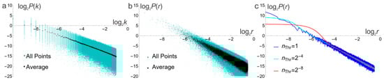
Figure 6. (a) ${\log }_2-{\log }_2$ plot of $P_{FT}\left(k,l_j\right), j:1\to 1025$ for a surface with $1025\times 1025$ points, together with the average for all 1025-line profiles. (b) Individual values and averages over all points with the same radius. (c) Filtered data. As the low-pass threshold radius $r_{Thr}$ decreases, dispersion is reduced, as is the linear part of the plot.

The data in Figure 6b present two inconveniences for correct regression analysis. The residual variance is not constant, and the density of data points increases strongly with r. Figure 6c shows the results of applying a low-pass filter to the average data of Figure 6b, with threshold radii $r_{Thr}=1,2^{-4},2^{-8}$. With the highest threshold, linearity is respected over the entire ${\log }_{2}r$ range, but dispersion is considerable for large values of r. As $r_{Thr}$ is increased, dispersion decreases, but the curve flattens for small $r_{Thr}$. This phenomenon is artificial and should not be confused with an upper cutoff. For the statistical simulations reported in Section 3.3, $r_{Thr}=2^{-5}$ was used, with linear regression performed for $r:2^{-6}\to 2^{-1}$.

An important aspect of PSA is illustrated in Figure 7. $P_{FT}\left(r\right)$ correctly reproduces the power-law PSD used as an input for FT. This is not a trivial result because the algorithm used to determine H by PSA does not “know” what kind of surface is used as an input, i.e., PSA does not use a trivial deconvolution of $\left\{\widehat{g_{ij}}\right\}$ and $P\left(r\right)$ because the input $\left\{\widehat{g_{ij}}\right\}$ are unknown to the algorithm. $P_{MP}\left(r\right)$ flattens at high frequencies. Although the theoretical analysis of MP shows that this method produces a power-law PSD [39], its numerical implementation induces a deviation of this theoretical behaviour. $P_{WM}\left(r\right)$ shows the strongest deviation from the ideal behaviour. The peaks in the spectrum are due to the finite values of N and M in Equation (3). Each peak corresponds to a circle of spikes in $P_{WM}\left(k,l\right)$ (Figure 2). Using PSA without accounting for this behaviour leads to large errors [32].

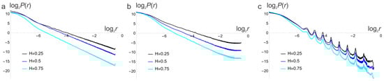
Figure 7. Filtered mean values of the ${\log }_2-{\log }_2$ plot for (a) $P_{FT}\left(r\right)$; (b) $P_{MP}\left(r\right)$; and (c) $P_{WM}\left(r\right)$.

2.9. Tuning of the SFA

A reference curve for the structure function $\gamma \left(r\right)$ can be calculated by eliminating C from Equations (1) and (2) and taking the limit for $r_u\to \infty$ for $P\left(r\right)$. This produces the following:

$$P\left(r\right)=\{\begin{array}{cc}0& r<r_l\\ \frac{<z^2>H{r}_l^{2H}}{\mathsf{\pi }}{r}^{-2\left(H+1\right)}& r_l\le r\end{array}$$

(14)

with the help of mathematical software, the IFT of Equation (14) can be found as the following:

$$\frac{R\left(\rho \right)}{<z^2>}=\frac{1}{<z^2>}{\mathcal{F}}^{-1}\left(P\left(r\right)\right)=-\frac{4^{-H}{r}_l^{2H}{\rho }^H\mathsf{\Gamma }\left(1-H\right)}{\mathsf{\Gamma }\left(1+H\right)}{+}_1{\mathrm{F}}_2\left(-H;1,1-H;-\frac{1}{4}{r}_l^2{\rho }^2\right),$$

(15)

where $\mathsf{\Gamma }(·)$ is the gamma function, and ₁F₂(·) is the generalised hypergeometric function. As $R\left(\rho \right)$ has zero crossings (Figure 8a), its representation in a ${\log }_2-{\log }_2$ plot is meaningless. The log–log plot for $\gamma \left(\rho \right)=1-R\left(\rho \right)$ shows asymptotic linear behaviour for ${\log }_2\rho <0$ (Figure 8b). Figure 8c shows the average of $\gamma \left(\rho \right)$ over all points with the same $\rho$ for H = 0.25, 0.5, 0.75 and $\mathcal{S}=FT$.

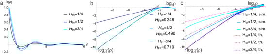
Figure 8. (a) presents $R\left(\rho \right)$ (Equation (15)) for H = 0.25, 0.5, 0.75, and $\mathcal{S}=FT$. (b) shows a ${\log }_2-{\log }_2$ plot of the theoretical value (Equation (15)), with linear fits (dashed) in the $\rho =2^{-10}-2^{-4}$ range. (c) shows the theoretical curves (th.) and simulated $\gamma \left(\rho \right)$ (sim.). The latter shows considerable horizontal offsets. Variations in H are much smaller but not negligible.

Contrary to the radial average of the PSD, no filtering is needed for SFA, but the range where the theoretical prediction and linear approach are valid is limited compared with the filtered PSD. There is a visible difference between the slope of the simulated $\gamma \left(\rho \right)$ and the theoretical curves. The horizontal offset of the simulated $\gamma \left(\rho \right)$ is a random value with broad dispersion. For calculating H, this offset is irrelevant.

3. Simulations and Results

3.1. Simulation Scheme

Five factors were considered in this study: the surface generating algorithm, the size of the dataset, the vertical scale ${\sigma }_0=\sqrt{<z^2{>}_{in}}$, the method for calculating H, and the value of H_in. The domain is defined as a grid of $2^{n_0}\times 2^{n_0}$ points, with $n_0$ taking values of 8, 9, and 10. An earlier study [49] showed that TPM, and to a lesser extent, DTF, depend on vertical scaling; three roughness values ${\sigma }_0$ equal to 0.25, 0.5, and 1 are considered. The methods used are DBC, TPM, DTF, PSA, SFA, and RLM.

The value of $H_{in}$ was varied from 1/128 to 127/128 in steps of 1/64. These values are chosen to exploit the perfectly parallel nature of the calculations on a processor with eight cores. Two surfaces were created for each combination of $\mathcal{S},$ $n_0$ and $H_{in}$. For each of these surfaces, the three values of ${\sigma }_0$ and all six methods were applied. The scheme allows the assessment of bias and dispersion by standard regression analysis and the comparison of results by ANOVA.

3.2. Data Analysis

For both $\mathcal{S}$, each $\mathcal{M}$ and $n_0$, $H_{\mathcal{S}\mathcal{M}}$ (or $H_{out}$) is plotted vs. $H_{in}$, for each value of ${\sigma }_0$. The linear regression is calculated with the following Equation:

$$H_{\mathcal{S}\mathcal{M}}=a_0+a_1{H}_{in}$$

(16)

is determined by standard least squares. A fourth regression line is estimated for the pooled data, disregarding the value of ${\sigma }_0$. The residual variance ${\sigma }_{Out}^2$ of the pooled data is compared with the mean residual variance of the three individual regression lines. The resulting F-ratio is compared with the 90% quantile of the F-distribution with the corresponding degrees of freedom, and the p-value is calculated. If p > 0.1, it is concluded that $\mathcal{M}$ is insensitive to ${\sigma }_0$ in the range evaluated.

The value of $a_1$ characterises the bias of the methods. Although this value cannot be studied entirely independently of $a_0$, $a_1$ affects the precision of a method. Having determined $H_{\mathcal{S}\mathcal{M}}$ (Equation (16)) and knowing $a_0$ and $a_1$, a corrected value can be found as the following:

$$H_{crr}=\frac{H_{\mathcal{S}\mathcal{M}}-a_0}{a_1}$$

(17)

${\sigma }_{out}$ represents the dispersion of the method. The precision of $\mathcal{M}$ can be defined as the difference between $H_{in}$ and $H_{crr}$ for a measured $H_{\mathcal{S}\mathcal{M}}$, quantified, for example, as the standard deviation between the predicted value $H_{crr}$ and $H_{in}$ is as follows:

$${\sigma }_{Pred}=\sqrt{<{\left(H_{in}-H_{crr}\right)}^2>}$$

(18)

${\sigma }_{out}$ interacts with $a_1$ in determining ${\sigma }_{Pred}$. Small values of $a_1$ magnify ${\sigma }_{out}$ when projected on the horizontal axis of the $H_{\mathcal{S}\mathcal{M}}$ vs. $H_{in}$-plot. ${\sigma }_{Pred}$ is obtained from the regression analysis on a $H_{in}$ vs. $H_{\mathrm{out}}$-plot, under the assumption that the residuals of this regression are independent of $H_{\mathcal{S}\mathcal{M}}$. If the residuals follow a normal distribution, the confidence intervals can be calculated. The assumption of normality was assessed using the Kolmogorov–Smirnov test.

3.3. Results for $\mathcal{S}=FT$

The complete results for $n_0$ = 10, ${\sigma }_0=$ 0.25, 0.5, and 1 and all $\mathcal{M}$ for $\mathcal{S}=FT$are presented in Figure 9. As an example, Table 1 presents the complete analysis of the regression results for DTF and DBC. For all $\mathcal{M}$, the regression results are independent of ${\sigma }_0$, although the $P_F$-values for TPM are close to 0.1. A summary of the pooled data for all $\mathcal{M}$ is shown in Table 2 and Table 3, for FT and MP and all $n_0$, together with $P_F$ and the 90% confidence interval for $H_{crr}$. None of the $P_{KM}$ indicate deviations from normality, but note that for $n_0$ = 8, $P_F=0.025$ for TPM, confirming its dependence on ${\sigma }_0$, as observed in an earlier study [49]. All methods except RLM and PSA present a visible increase in the variance with $H_{in}$. This effect is not studied in detail and is neglected in the statistical analysis.

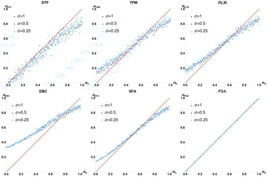
Figure 9. Plots of $H_{FT\mathcal{M}}$ vs. $H_{in}$ for three values of ${\sigma }_0$ and all $\mathcal{M}$, with the ideal case $H_{FT\mathcal{M}}=H_{in}$ marked as a red line. The methods are listed in order the precision ${\sigma }_{Pred}$.

Table 1. Results of the regression analysis for $n_0$ = 10, ${\sigma }_0=$ 0.25, 0.5, and 1 for $\mathcal{S}=FT$ and $\mathcal{M}=DTF$ and DBC. The first three lines present the results for individual ${\sigma }_0$. R² is the coefficient of determination, and n is the number of simulations. The next line presents the results for the pooled values. Line 6 presents the ANOVA results for the effect of ${\sigma }_0$; F_90% and $P_{{\sigma }_0}$ are the 90% confidence level and p-value for the Fisher test, respectively. Line 8 gives the residual standard deviation ${\sigma }_{Pred}$, the 90% confidence interval for $H_{crr},$ and the p-value for the Kolmogorov–Smirnov test ($P_{KM}$) applied to the residuals of the $H_{in}$ vs. $H_{\mathcal{S}\mathcal{M}}$ regression line.

DTF	a0	a1	sout	R2	n
${\sigma }_0=1$	0.014	0.848	0.046	0.968	128
${\sigma }_0=0.5$	0.002	0.852	0.046	0.968	128
${\sigma }_0=0.25$	0.002	0.866	0.044	0.972	128
Pooled	0.006	0.855	0.045	0.969	384
$\mathrm{ANOVA} {\sigma }_0$	F-ratio	F90%	$P_{{\sigma }_0}$
	1.011	1.139	0.458
Precision	sPred	90% CI	PKM
	0.052	±0.087	0.755
DBC	a0	a1	σout	R2	n
${\sigma }_0=1$	0.308	0.594	0.016	0.992	128
${\sigma }_0=0.5$	0.305	0.601	0.018	0.99	128
${\sigma }_0=0.25$	0.306	0.598	0.018	0.99	128
Pooled	0.306	0.597	0.017	0.991	384
ANOVA σ	F-ratio	F90%	$P_{{\sigma }_0}$
	1.003	1.139	0.488
Precision	σPred	90% CI	PKM
	0.028	±0.048	0.97

Table 2. Summary of the statistical results for $\mathcal{S}=FT$ and all $\mathcal{M}$. The results are pooled over all ${\sigma }_0$. Notice how ${\sigma }_{out}$ and the 90% CI on $H_{crr}$ increase with decreasing $n_0$.

Method	${\mathit{n}}_0$	a0	a1	σout	R2	${\mathit{P}}_{{\mathit{\sigma }}_0}$	90% CI
DTF	10	0.002	0.866	0.044	0.972	0.458	±0.087
	9	−0.004	0.841	0.049	0.962	0.458	±0.105
	8	0.002	0.845	0.069	0.927	0.494	±0.13
TPM	10	0.137	0.744	0.03	0.982	0.11	±0.067
	9	0.153	0.716	0.033	0.976	0.15	±0.078
	8	0.175	0.691	0.039	0.964	0.025	±0.095
RLM	10	0.144	0.741	0.024	0.988	0.487	±0.053
	9	0.155	0.723	0.025	0.986	0.472	±0.06
	8	0.182	0.692	0.029	0.979	0.481	±0.071
DBC	10	0.306	0.597	0.017	0.991	0.488	±0.048
	9	0.338	0.559	0.018	0.988	0.442	±0.053
	8	0.375	0.52	0.023	0.978	0.489	±0.074
SFA	10	0.107	0.787	0.016	0.995	0.487	±0.034
	9	0.128	0.758	0.018	0.993	0.491	±0.039
	8	0.153	0.726	0.018	0.993	0.479	±0.042
PSA	10	0.001	1.001	0.002	1	0.4134	±0.0032
	9	0.003	1.001	0.004	1	0.4984	±0.0068
	8	0.007	1.007	0.008	0.999	0.4692	±0.0137

Table 3. Summary of the statistical results for $\mathcal{S}=MP$ and all $\mathcal{M}$. The results are pooled over all ${\sigma }_0$. Generally, bias is higher, and precision is lower than in FT.

Method	${\mathit{n}}_0$	a0	a1	σout	R2	${\mathit{P}}_{{\mathit{\sigma }}_0}$	90% CI
DTF	10	−0.014	0.884	0.047	0.967	0.004	±0.089
	9	−0.028	0.874	0.05	0.962	0.008	±0.077
	8	−0.042	0.86	0.062	0.942	0.011	±0.064
TPM	10	0.034	0.893	0.029	0.988	0.015	±0.083
	9	0.033	0.889	0.034	0.983	0.023	±.064
	8	0.045	0.859	0.04	0.975	0.027	±0.077
RLM	10	0.014	0.922	0.021	0.994	0.468	±0.039
	9	0.013	0.917	0.024	0.992	0.477	±.044
	8	0.017	0.901	0.032	0.985	0.415	±0.06
DBC	10	0.268	0.641	0.018	0.99	0.488	±0.05
	9	0.3	0.599	0.021	0.986	0.479	±0.059
	8	0.339	0.546	0.025	0.975	0.376	±0.079
SFA	10	0.148	0.549	0.047	0.919	0.466	±0.036
	9	0.155	0.535	0.043	0.929	0.486	±0.049
	8	0.165	0.511	0.037	0.943	0.488	±0.062
PSA	10	−0.065	1.038	0.013	0.998	0.446	±0.022
	9	−0.059	1.046	0.02	0.996	0.485	±0.033
	8	−0.033	1.056	0.03	0.99	0.47	±0.048

3.4. Results for $\mathcal{S}=MP$

The results for $\mathcal{S}=MP$ differ considerably from $\mathcal{S}=FT$. Figure 10 shows that SFA has a large bias, especially for high values of H (low D), where the predominance of the first few values in MP is not masked by the strong fluctuations associated with low H. In the statistical results (Table 3), the precision for $H_{TPM}$ and $H_{DBC}$ varies significantly with ${\sigma }_0$, as found in an earlier study [49]. This effect depends on both the surface simulation method and the algorithm used for the calculation of D.

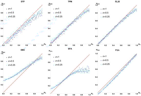
Figure 10. Plots of $H_{MP\mathcal{M}}$ vs. $H_{in}$ for three values of ${\sigma }_0$ and all $\mathcal{M}$. For DTF and TPM, the results depend significantly on ${\sigma }_0$; for DBC and SFA, the bias is much higher than in $H_{FT\mathcal{M}}$.

4. Discussion

4.1. Bias, Dispersion, and Precision

Most studies on the fractal dimension of measured data conclude that different methods yield different results, as is clearly confirmed here. However, if the exact input value $H_{in}$ is a priori unknown, there is no way to decide which $H_{\mathcal{S}\mathcal{M}}$ is closer to this value. In the field of image recognition, there is a tradition of applying different methods to a standard library of bitmaps and evaluating whether a method can distinguish between similar images [23,24,25,51]. Methods are then compared based on their consistency with earlier research, but such an approach does not provide information on bias or statistical dispersion.

Using simulated data with known $H_{in}$, two factors become clear at once. The first is the bias $B\left(H_{in}\right)$, as captured by $a_1$. DBC is clearly underperforming in this regard. However, by Equation (17), this can be corrected by if $a_0$ and $a_1$ are calibrated through numerical simulation. Dispersion (σ_out) cannot be corrected. In this aspect, DBC outperforms the other methods, except for PSA. σ_out combines with B to determine ${\sigma }_{Pred}$ and the confidence interval for $H_{crr}$. A low value of $a_1$ will magnify the dispersion on $H_{crr}$ for a given $H_{out}$. The low dispersion found in DBC cancels out the effect of bias for $\mathcal{S}=PS$. This effect has not received due attention in the literature; most studies comparing different methods for the determination of D do not define precision.

4.2. Computational Efficiency

In the context of this study, efficiency can be interpreted either in terms of computational speed or the optimal use of information. Computation speed is often a secondary concern if the effort involved in measuring $z\left(x,y\right)$ is much greater than the work involved in the calculation of D. However, as the size of the datasets increases, the computational cost may blow up. In applications such as real-time pattern recognition, computational speed is essential. PSA, DBC, and RLM will have an advantage here.

To compare computational efficiency, it must be ensured that the most efficient algorithm is used for each method. A straightforward example is the use of FFT in SFA and PSA, but efficient algorithms are also known for BCM [68] and direct calculation of $R\left(\rho \right)$ and $\gamma \left(\rho \right)$ [69]. As the algorithms in this study have not been fully optimised for efficiency, only the most evident effects will be mentioned. As an example, the full PSA routine used here for $n_0=10$ takes 5″ using a single core on an 11th Gen Intel Core i9-11950H @ 2.60 GHz. Additional software optimisation can certainly increase this speed.

Calculation of the cumulative function in DTF and of the variance in RLM can be significantly sped up using the results at length scale a to obtain the values for 2a. A naive calculation of $z^2$ was used in RLM because, even without optimisation, this method is very fast. In contrast, DTF blows up rapidly with $n_0$. The use of the cumulative function instead of the original values, combined with a regression analysis for each subset in each step, generates computational overhead. TPM is not very efficient either and is not very precise.

Further development of DTF and TPM to analyse physical measurements in the form of $z\left(x_i,y_j\right)$ shows little promise. Considering the algorithms used in this study, DBC, RLM, PSA, and SFA are at least ten times more efficient than TPM, which is significantly faster than DTF. SFA takes about twice the time of PSA simply because of the calculation of the IFT in addition to the FFT. Given the lower precision of SFA, PSA is preferred.

4.3. Information Efficiency

Information efficiency describes how much of the available information in the dataset is effectively used to estimate D, including the individual values of $z\left(x_i,y_j\right)$ and their spatial correlation. Power spectral analysis and autocorrelation were originally developed for the analysis of time series. Contact surface profilers measure roughness along a line [3]; hence, estimating fractal dimensions by analysing data along a line is a deep-rooted tradition [61,63,70,71].

Most modern applications generate large datasets over a rectangular array of regularly spaced points, as is the case for images obtained by digital cameras, atomic force microscopes, optical roughness measurements, or photogrammetry data. To analyse single lines out of a full set of $f\left(x_i,y_j\right)$ data induces a considerable loss of information and may even distort the conclusions of the analysis [72,73]. The effect is clearly illustrated in Figure 6a, where the power spectrum of single lines shows extreme dispersion, but the average value of the 1025 lines appears as a well-defined straight line. Single-line analysis should never be performed if data are available over a 2D domain.

Even so, DTF, TPM, DBC, and RLM do not use all available information because they are typically implemented by subsequent division of intervals by two in each step. For the periodic surfaces generated by FT, there are $2^{2n_0}$ possible positions to collocate the corner of the first interval. While the computational cost of DTF and TPM does not encourage exploration of this effect, it has been used to decrease the statistical dispersion in DBC [20,21,51] and can be used in RLM. According to the definition of the Minkowski dimension [20], in DBC, the infimum of $n_m$ should be determined, while in RLM, the mean value can be used. Calculating all possible values would significantly increase the calculation time for RLM and DBC. SFA and PSA are not subject to this observation.

4.4. Effect of Vertical Scaling and Resolution

Vertical scaling clearly affects TPM but was found to be insignificant in all other methods for FT. It also affects DTF for MP. It is always possible to apply vertical rescaling such that ${\sigma }_0$ is of the same order of ${\lambda }_u$ if the significant number of digits for x, y, and z is equal, i.e., image depth should be equal to image resolution [49]. If not, scaling only increases the gaps between consecutive vertical values. Many scientific cameras obey this condition, and optical roughness measurements often have a higher vertical resolution than lateral resolution. In numerical simulations, the vertical resolution is limited by machine precision, while the lateral resolution is defined by $n_0$.

In terms of cameras and measurement systems available in many laboratory settings, $n_0=10$ is rather modest. However, for time-consuming measurements, large sample sets, or computationally complex simulations, it may still be interesting to work at lower $n_0$. It follows from Table 2 and Table 3 that ${\sigma }_{out}$ increases with decreasing $n_0$. The effect is small for all methods except for PSA, where the increase in ${\sigma }_{out}$ is proportional to the reduction in spatial resolution. Still, at $n_0=8$, PSA outperforms all other methods at $n_0=10$, i.e., better estimates can be obtained using smaller datasets.

4.5. Effect of the Surface Generation Algorithm

PSA is more precise than the other methods for FT by a factor of 10. $P_{FT}\left(r\right)$ is related to the input function $P\left(r\right)$ in Equation (4) by $\left\{\widehat{g_{ij}}\right\}$, which randomises the result. It has been claimed that using PSA with $\mathcal{S}=FT$ is “unfair” [32] because one is presumably the inverse of the other. It was pointed out in Section 2.8 that this is not the case; the implementation of PSA used in this work is independent of the surface generating algorithm. The excellent results obtained by PSA from surfaces generated by FT show that both methods are consistent.

The radial PS of surfaces defined by MP has a reduced linear section in the log–log plot (Figure 7). DTF is slightly more successful here than for $\mathcal{S}=FT$ (Table 2 and Table 3) because the principal characteristic of DTF is to filter out effects of nonstationarity, which is inherent to MP [37]. Zhang et al. [32] detected a breakdown of PSA for WM. This can be associated with the discrete peaks in the PS (Figure 2b and Figure 7c). These peaks are the reason why WM was not included in the analysis, as they do not appear in the experimental spectra available in the literature [12,13,14,15,16,17,18].

As a reference, a series of simulations was performed for WM with $n_0=10$ using RLM and PSA. The latter method does not produce useful results over the entire range of H. RLM gave $H_{WM RLM}=0.082+0.81H_{in}$, with ${\sigma }_{out}=0.02$. This is comparable to RLM and SFA for FT. It follows that an approximate value for H can be obtained, even if the initial assumption (Equation (1)) is not fulfilled. Without the analysis of the PS, the peaks in the PS for WM would be overlooked. An extensive statistical analysis of the available surface generation algorithms, in terms of their PS, H, and the probability density distribution of surface heights, is an interesting topic for future investigation.

If the purpose of a study is to simulate a surface which conforms to Equation (1), the peaks in the PS created by WM induce a deviation from the basic hypothesis. Whether such preferred frequencies are important in the simulation depends on the application. For optical phenomena, they can be very important as they may interact with the frequency of the optical signal. In contact and fracture mechanics, the effect of the details of the PS has not been critically analysed. MP introduces a smaller deviation than WM, but its effect on specific applications has not been quantified either.

If the goal is to estimate the fractal dimension of some measured dataset $z=z\left(x,y\right)$, it is important to investigate whether the hypothesis of a power-law PS is fulfilled. This can be carried out by plotting $P\left(\sqrt{k^2+l^2}\right)$ as in Figure 7 or by studying the residual standard deviation and coefficient of determination of the linear fit to the ${\log }_2-{\log }_2$ plot for $P\left(r\right)$. Failure to do so may lead to incorrect or incomplete conclusions about the character of the data.

The simulations made in this work are meant as a reference for the analysis of experimental data. In an experimental setting, D is a priory unknown, so it is not possible to compare and calibrate the methods objectively. For measurements on an irregular grid, the present version of PSA is not feasible, and other methods may be selected. For experimental results on a regular grid, which may show deviations from the exact power law (Equation (1)), PSA can detect such deviations, while techniques such as DBC and DTF will mask them, which may represent an unacceptable loss of information.

Refined methods for the characterisation of more complex random processes on a two-dimensional domain can be devised. Substituting the simple power law by more advanced fitting functions may be the first approach to this problem. For the simulation of surfaces which purposedly deviate from Equation (1), the FT technique can use more refined expressions for $P\left(k,l\right)$ in Equation (4).

5. Conclusions

A basic rule in scientific research is that measurement techniques must be calibrated to reliable standards. Neither calibration techniques nor standards have been clearly defined for determining the Hurst exponent of random fractal surfaces defined as $z=z\left(x,y\right)$ on a unit square. This study defines the bias, dispersion, and precision of the methods. Bias refers to the difference between the output and input values of the Hurst exponent. It is a function of the deterministic input value $H_{in}$. Dispersion is the standard deviation of the random variable $H_{out}$, and precision is the standard deviation after correction for bias, i.e., on $H_{crr}$.

The consistency and high precision of the power spectral analysis for surfaces produced by the Fourier transform method establishes the latter as a useful standard for the other methods. The detrended fluctuation and triangular prism methods can be rejected because of their computational cost and low precision. Based on the bias, differential box counting should be rejected. Box counting methods were developed to characterise contours $z_0=z\left(x,y\right)$ in the plane but not for surfaces $z=z\left(x,y\right)$ in three dimensions, where they underperform.

Differential box counting and detrended fluctuation can filter out deviations of the perfect power law behaviour of the power spectrum, but power spectral analysis accurately detects these deviations. Future research should, therefore, focus on exploring the unique capabilities of power spectral analysis, rather than trying to improve methods that are computationally inefficient or make suboptimal use of the information available in the measurements.

References

- Longuet-Higgins, M.S. The statistical analysis of a random, moving surface. Philos. Trans. R. Soc. Lond. Ser. A Math. Phys. Sci. 1957, 249, 321–387. [Google Scholar] [CrossRef]
- Longuet-Higgins, M.S. Statistical properties of an isotropic random surface. Philos. Trans. R. Soc. Lond. Ser. A Math. Phys. Sci. 1957, 250, 157–174. [Google Scholar] [CrossRef]
- Whitehouse, D.J.; Archard, J.F. The properties of random surfaces of significance in their contact. Proc. R. Soc. Lond. Ser. A. Math. Phys. Sci. 1970, 316, 97–121. [Google Scholar] [CrossRef]
- Pfeifer, P. Fractal dimension as working tool for surface-roughness problems. Appl. Surf. Sci. 1984, 18, 146–164. [Google Scholar] [CrossRef]
- Pfeifer, P.; Wu, Y.J.; Cole, M.W.; Krim, J. Multilayer adsorption on a fractally rough surface. Phys. Rev. Lett. 1989, 62, 1997–2000. [Google Scholar] [CrossRef]
- Wang, C.L.; Krim, J.; Toney, M.F. Roughness and porosity characterization of carbon and magnetic films through adsorption isotherm measurements. J. Vac. Sci. Technol. A 1989, 7, 2481–2485. [Google Scholar] [CrossRef]
- Majumdar, A.; Bhushan, B. Role of Fractal Geometry in Roughness Characterization and Contact Mechanics of Surfaces. J. Tribol. 1990, 112, 205–216. [Google Scholar] [CrossRef]
- Mandelbrot, B.B. The Fractal Geometry of Nature; WH Freeman: New York, NY, USA, 1982. [Google Scholar]
- Richardson, L.F. The problem of contiguity: An appendix to statistics of deadly quarrels. Gen. Syst. Yearb. 1961, 6, 139–187. [Google Scholar]
- Mandelbrot, B. How long is the coast of Britain? Statistical self-similarity and fractional dimension. Science 1967, 156, 636–638. [Google Scholar] [CrossRef]
- Plancherel, M.; Leffler, M. Contribution à ľétude de la représentation d’une fonction arbitraire par des intégrales définies. Rend. Circ. Mat. Palermo (1884–1940) 1910, 30, 289–335. [Google Scholar] [CrossRef]
- Gujrati, A.; Khanal, S.R.; Pastewka, L.; Jacobs, T.D.B. Combining TEM, AFM, and profilometry for quantitative topography characterization across all scales. ACS Appl. Mater. Interfaces 2018, 10, 29169–29178. [Google Scholar] [CrossRef] [PubMed]
- Gujrati, A.; Sanner, A.; Khanal, S.R.; Moldovan, N.; Zeng, H.; Pastewka, L.; Jacobs, T.D.B. Comprehensive topography characterization of polycrystalline diamond coatings. Surf. Topogr. Metrol. Prop. 2021, 9, 014003. [Google Scholar] [CrossRef]
- Philcox, O.H.E.; Torquato, S. Disordered Heterogeneous Universe: Galaxy Distribution and Clustering across Length Scales. Phys. Rev. X 2023, 13, 011038. [Google Scholar] [CrossRef]
- Smith, M.W. Roughness in the Earth Sciences. Earth-Sci. Rev. 2014, 136, 202–225. [Google Scholar] [CrossRef]
- Pardo-Igúzquiza, E.; Dowd, P.A. Fractal analysis of the Martian landscape: A study of kilometre-scale topographic roughness. Icarus 2022, 372, 114727. [Google Scholar] [CrossRef]
- Pardo-Igúzquiza, E.; Dowd, P.A. The roughness of Martian topography: A metre-scale fractal analysis of six selected areas. Icarus 2022, 384, 115109. [Google Scholar] [CrossRef]
- Persson, B.N.J. On the fractal dimension of rough surfaces. Tribol. Lett. 2014, 54, 99–106. [Google Scholar] [CrossRef]
- Theiler, J. Estimating fractal dimension. J. Opt. Soc. Am. A 1990, 7, 1055–1073. [Google Scholar] [CrossRef]
- Falconer, K. Fractal Geometry: Mathematical Foundations and Applications; John Wiley & Sons: Hoboken, NJ, USA, 2004. [Google Scholar]
- Bandt, C.; Hung, N.; Rao, H. On the open set condition for self-similar fractals. Proc Amer. Math. Soc. 2006, 134, 1369–1374. [Google Scholar] [CrossRef]
- Panigrahy, C.; Seal, A.; Mahato, N.K. Quantitative texture measurement of gray-scale images: Fractal dimension using an improved differential box counting method. Measurement 2019, 147, 106859. [Google Scholar] [CrossRef]
- Nayak, S.R.; Mishra, J. An improved method to estimate the fractal dimension of colour images. Perspect. Sci. 2016, 8, 412–416. [Google Scholar] [CrossRef]
- Nayak, S.R.; Mishra, J.; Palai, G. Analysing roughness of surface through fractal dimension: A review. Image Vis. Comput. 2019, 89, 21–34. [Google Scholar] [CrossRef]
- Liang, H.; Tsuei, M.; Abbott, N.; You, F. AI framework with computational box counting and Integer programming removes quantization error in fractal dimension analysis of optical images. Chem. Eng. J. 2022, 446, 137058. [Google Scholar] [CrossRef]
- Coles, P.; Barrow, J.D. Non-Gaussian statistics and the microwave background radiation. Mon. Not. R. Astron. Soc. 1987, 228, 407–426. [Google Scholar] [CrossRef]
- Heavens, A.F.; Sheth, R.K. The correlation of peaks in the microwave background. Mon. Not. R. Astron. Soc. 1999, 310, 1062–1070. [Google Scholar] [CrossRef][Green Version]
- Wang, R.; Singh, A.K.; Kolan, S.R.; Tsotsas, E. Fractal analysis of aggregates: Correlation between the 2D and 3D box-counting fractal dimension and power law fractal dimension. Chaos Solitons Fractals 2022, 160, 112246. [Google Scholar] [CrossRef]
- Florindo, J.B.; Bruno, O.M. Closed contour fractal dimension estimation by the Fourier transform. Chaos Solitons Fractals 2011, 44, 851–861. [Google Scholar] [CrossRef]
- Ausloos, M.; Berman, D.H. A multivariate Weierstrass–Mandelbrot function. Proc. R. Soc. Lond. Ser. A. Math. Phys. Sci. 1985, 400, 331–350. [Google Scholar] [CrossRef]
- Yan, W.; Komvopoulos, K. Contact analysis of elastic-plastic fractal surfaces. J. Appl. Phys. 1998, 84, 3617–3624. [Google Scholar] [CrossRef]
- Zhang, X.; Xu, Y.; Jackson, R.L. An analysis of generated fractal and measured rough surfaces in regards to their multi-scale structure and fractal dimension. Tribol. Int. 2017, 105, 94–101. [Google Scholar] [CrossRef]
- Xiao, H.; Sun, Y.; Chen, Z. Fractal modeling of normal contact stiffness for rough surface contact considering the elastic–plastic deformation. J. Braz. Soc. Mech. Sci. Eng. 2019, 41, 11. [Google Scholar] [CrossRef]
- Wei, D.; Zhai, C.; Hanaor, D.; Gan, Y. Contact behaviour of simulated rough spheres generated with spherical harmonics. Int. J. Solids Struct. 2020, 193–194, 54–68. [Google Scholar] [CrossRef]
- Yu, X.; Sun, Y.; Zhao, D.; Wu, S. A revised contact stiffness model of rough curved surfaces based on the length scale. Tribol. Int. 2021, 164, 107206. [Google Scholar] [CrossRef]
- Liu, L.; Shi, Y.; Hu, F. Application of the Weierstrass–Mandelbrot function to the simulation of atmospheric scalar turbulence: A study for carbon dioxide. Fractals 2022, 30, 2250086. [Google Scholar] [CrossRef]
- Kant, K.; Sibin, K.; Pitchumani, R. Novel fractal-textured solar absorber surfaces for concentrated solar power. Sol. Energy Mater. Sol. Cells 2022, 248, 112010. [Google Scholar] [CrossRef]
- Shen, F.; Li, Y.-H.; Ke, L.-L. A novel fractal contact model based on size distribution law. Int. J. Mech. Sci. 2023, 249, 108255. [Google Scholar] [CrossRef]
- Saupe, D. Algorithms for random fractals. In The Science of Fractal Images; Peitgen, H.O., Saupe, D., Eds.; Springer: New York, NY, USA, 1988; pp. 71–136. [Google Scholar]
- Lam, N.S.-N.; Qiu, H.-L.; Quattrochi, D.A.; Emerson, C.W. An evaluation of fractal methods for characterizing image complexity. Cartogr. Geogr. Inf. Sci. 2002, 29, 25–35. [Google Scholar] [CrossRef]
- Zhou, G.; Lam, N.S.-N. A comparison of fractal dimension estimators based on multiple surface generation algorithms. Comput. Geosci. 2005, 31, 1260–1269. [Google Scholar] [CrossRef]
- Burger, H.; Forsbach, F.; Popov, V.L. Boundary Element Method for Tangential Contact of a Coated Elastic Half-Space. Machines 2023, 11, 694. [Google Scholar] [CrossRef]
- Yastrebov, V.A.; Anciaux, G.; Molinari, J.-F. The role of the roughness spectral breadth in elastic contact of rough surfaces. J. Mech. Phys. Solids 2017, 107, 469–493. [Google Scholar] [CrossRef]
- Hu, Y.Z.; Tonder, K. Simulation of 3-D random rough surface by 2-D digital filter and Fourier analysis. Int. J. Mach. Tools Manuf. 1992, 32, 83–90. [Google Scholar] [CrossRef]
- Yastrebov, V.A.; Anciaux, G.; Molinari, J.-F. From infinitesimal to full contact between rough surfaces: Evolution of the contact area. Int. J. Solids Struct. 2015, 52, 83–102. [Google Scholar] [CrossRef]
- Foroutan-Pour, K.; Dutilleul, P.; Smith, D. Advances in the implementation of the box-counting method of fractal dimension estimation. Appl. Math. Comput. 1999, 105, 195–210. [Google Scholar] [CrossRef]
- Wu, J.; Jin, X.; Mi, S.; Tang, J. An effective method to compute the box-counting dimension based on the mathematical definition and intervals. Results Eng. 2020, 6, 100106. [Google Scholar] [CrossRef]
- So, G.-B.; So, H.-R.; Jin, G.-G. Enhancement of the Box-Counting Algorithm for fractal dimension estimation. Pattern Recognit. Lett. 2017, 98, 53–58. [Google Scholar] [CrossRef]
- Schouwenaars, R.; Jacobo, V.H.; Ortiz, A. The effect of vertical scaling on the estimation of the fractal dimension of randomly rough surfaces. Appl. Surf. Sci. 2017, 425, 838–846. [Google Scholar] [CrossRef]
- Wu, M.; Wang, W.; Shi, D.; Song, Z.; Li, M.; Luo, Y. Improved box-counting methods to directly estimate the fractal dimension of a rough surface. Measurement 2021, 177, 109303. [Google Scholar] [CrossRef]
- Liu, C.; Zhan, Y.; Deng, Q.; Qiu, Y.; Zhang, A. An improved differential box counting method to measure fractal dimensions for pavement surface skid resistance evaluation. Measurement 2021, 178, 109376. [Google Scholar] [CrossRef]
- Gneiting, T.; Ševčíková, H.; Percival, D.B. Estimators of fractal dimension: Assessing the roughness of time series and spatial data. Stat. Sci. 2012, 27, 247–277. [Google Scholar] [CrossRef]
- Hall, P.; Wood, A. On the performance of box-counting estimators of fractal dimension. Biometrika 1993, 80, 246–251. [Google Scholar] [CrossRef]
- Clarke, K.C. Computation of the fractal dimension of topographic surfaces using the triangular prism surface area method. Comput. Geosci. 1986, 12, 713–722. [Google Scholar] [CrossRef]
- De Santis, A.; Fedi, M.; Quarta, T. A revisitation of the triangular prism surface area method for estimating the fractal dimension of fractal surfaces. Ann. Geophys. 1997, 15, 811–821. [Google Scholar] [CrossRef]
- Kantelhardt, J.W.; Zschiegner, S.A.; Koscielny-Bunde, E.; Havlin, S.; Bunde, A.; Stanley, H. Multifractal detrended fluctuation analysis of nonstationary time series. Phys. A Stat. Mech. Its Appl. 2002, 316, 87–114. [Google Scholar] [CrossRef]
- Gu, G.-F.; Zhou, W.-X. Detrended fluctuation analysis for fractals and multifractals in higher dimensions. Phys. Rev. E 2006, 74, 061104. [Google Scholar] [CrossRef]
- Gu, G.-F.; Zhou, W.-X. Detrending moving average algorithm for multifractals. Phys. Rev. E 2010, 82, 011136. [Google Scholar] [CrossRef]
- Malinverno, A. A simple method to estimate the fractal dimension of a self-affine series. Geophys. Res. Lett. 1990, 17, 1953–1956. [Google Scholar] [CrossRef]
- Kulatilake, P.H.S.W.; Ankah, M.L.Y. Rock Joint Roughness Measurement and Quantification—A Review of the Current Status. Geotechnics 2023, 3, 116–141. [Google Scholar] [CrossRef]
- Wen, R.; Sinding-Larsen, R. Uncertainty in fractal dimension estimated from power spectra and variograms. Math. Geol. 1997, 29, 727–753. [Google Scholar] [CrossRef]
- Kondev, J.; Henley, C.L.; Salinas, D.G. Nonlinear measures for characterizing rough surface morphologies. Phys. Rev. E 2000, 61, 104–125. [Google Scholar] [CrossRef]
- Jiang, K.; Liu, Z.; Tian, Y.; Zhang, T.; Yang, C. An estimation method of fractal parameters on rough surfaces based on the exact spectral moment using artificial neural network. Chaos Solitons Fractals 2022, 161, 112366. [Google Scholar] [CrossRef]
- Bhushan, B. Surface roughness analysis and measurement techniques. In Modern Tribology Handbook; Bhushan, B., Ed.; two volume set; CRC Press: Boca Raton, FL, USA, 2000. [Google Scholar]
- Cheng, Q.; Agterberg, F. Fractal Geometry in Geosciences. In Encyclopedia of Mathematical Geosciences; Springer International Publishing: Cham, Switzerland, 2022; pp. 1–24. [Google Scholar]
- Wang, H.; Chi, G.; Jia, Y.; Ge, C.; Yu, F.; Wang, Z.; Wang, Y. Surface roughness evaluation and morphology reconstruction of electrical discharge machining by frequency spectral analysis. Measurement 2020, 172, 108879. [Google Scholar] [CrossRef]
- Eftekhari, L.; Raoufi, D.; Eshraghi, M.J.; Ghasemi, M. Power spectral density-based fractal analyses of sputtered yttria-stabilized zirconia thin films. Semicond. Sci. Technol. 2022, 37, 105011. [Google Scholar] [CrossRef]
- Kruger, A. Implementation of a fast box-counting algorithm. Comput. Phys. Commun. 1996, 98, 224–234. [Google Scholar] [CrossRef]
- Marcotte, D. Fast variogram computation with FFT. Comput. Geosci. 1996, 22, 1175–1186. [Google Scholar] [CrossRef]
- Zuo, X.; Peng, M.; Zhou, Y. Influence of noise on the fractal dimension of measured surface topography. Measurement 2020, 152, 107311. [Google Scholar] [CrossRef]
- Wu, J.-J. Structure function and spectral density of fractal profiles. Chaos Solitons Fractals 2001, 12, 2481–2492. [Google Scholar] [CrossRef]
- Nayak, P.R. Random Process Model of Rough Surfaces. J. Lubr. Technol. 1971, 93, 398–407. [Google Scholar] [CrossRef]
- Greenwood, J.A. A unified theory of surface roughness. Proc. R. Soc. Lond. Ser. A. Math. Phys. Sci. 1984, 393, 133–157. [Google Scholar] [CrossRef]
Disclaimer/Publisher’s Note: The statements, opinions and data contained in all publications are solely those of the individual author(s) and contributor(s) and not of MDPI and/or the editor(s). MDPI and/or the editor(s) disclaim responsibility for any injury to people or property resulting from any ideas, methods, instructions or products referred to in the content. |
© 2024 by the authors. Licensee MDPI, Basel, Switzerland. This article is an open access article distributed under the terms and conditions of the Creative Commons Attribution (CC BY) license (https://creativecommons.org/licenses/by/4.0/).