Minimal Wave Speed for a Nonlocal Viral Infection Dynamical Model

Abstract

To provide insights into the spreading speed and propagation dynamics of viruses within a host, in this paper, we investigate the traveling wave solutions and minimal wave speed for a degenerate viral infection dynamical model with a nonlocal dispersal operator and saturated incidence rate. It is found that the minimal wave speed $c^{\ast }$ is the threshold that determines the existence of traveling wave solutions. The existence of traveling fronts connecting a virus-free steady state and a positive steady state with wave speed $c\ge c^{\ast }$ is established by using Schauder’s fixed-point theorem, limiting arguments, and the Lyapunov functional. The nonexistence of traveling fronts for $c<c^{\ast }$ is proven by the Laplace transform. In particular, the lower-bound estimation of the traveling wave solutions is provided by adopting a rescaling method and the comparison principle, which is a crucial prerequisite for demonstrating that the traveling semifronts connect to the positive steady state at positive infinity by using the Lyapunov method and is a challenge for some nonlocal models. Moreover, simulations show that the asymptotic spreading speed may be larger than the minimal wave speed and the spread of the virus may be postponed if the diffusion ability or diffusion radius decreases. The spreading speed may be underestimated or overestimated if local dispersal is adopted.

1. Introduction

Although huge advances have been made in preventing and treating HIV and viral hepatitis, such as antiretroviral treatment for HIV and vaccination programs for the hepatitis B virus (HBV), HIV and HBV pandemics remain a major global public health problem. It is reported that there were $36.9$ million people living with HIV worldwide in 2017 and 257 million people and 71 million people in 2015 were living with HBV and hepatitis C virus (HCV), respectively. Meanwhile, $0.94$ million people in 2017 and $1.3$ million people in 2015 died from AIDS-related and hepatitis-related illnesses, respectively [1,2]. Therefore, we have a long way to go to control and extinguish these viral infectious diseases.

To understand the pathogenesis of viruses within the host and then propose more effective control measures, many different methods have been developed. In particular, mathematical models have been verified as an effective method [3,4]. In 2000, Nowak and May [5] proposed the following basic viral infection model:

$$\left\{\begin{array}{c}\frac{dw(t)}{dt}=s-bw(t)-\beta w(t)v(t),\hfill \\ \frac{du(t)}{dt}=\beta w(t)v(t)-\mu u(t),\hfill \\ \frac{dv(t)}{dt}=pu(t)-\gamma v(t),\hfill \end{array}\right.$$

(1)

where $w(t)$, $u(t)$, and $v(t)$ denote the concentrations of healthy target cells, infected cells, and free virions at time t, respectively. s is the recruitment rate of healthy target cells. b, $\mu$, and $\gamma$ represent the death rates of healthy target cells, infected cells, and free virions, respectively. The infectious incidence rate is $\beta w(t)v(t)$ and p is the virus production rate. All the parameters in model (1) are positive. System (1) has a virus-free equilibrium point $E_0=(w_0,0,0)$, which is globally asymptotically stable when ${\mathcal{R}}_0\le 1$, where $w_0=s/b$ and ${\mathcal{R}}_0=p\beta s/(b\mu \gamma )=p\beta w_0/(\mu \gamma )$. If ${\mathcal{R}}_0>1$, system (1) admits at a unique positive equilibrium point that is globally asymptotically stable [6]. Since then, many works concerning the impacts of various factors on within-host viral dynamics have been conducted using mathematical models [7,8]. Although the incidence rate in most of these viral models adopts a bilinear function response, this may be not so appropriate when the concentration of virions is high. In this case, the saturation effect may cause a viral response rate that is less than linear. Hence, it is more reasonable to adopt a saturation nonlinear incidence rate $\beta w(t)v^m(t)/(1+\alpha v^n(t))$, where $m,n,\alpha >0$. The case where $m=n=1$ has been studied in viral infection models by several researchers, including [9,10].

Note that many studies on viral infection models assume that the within-host environments are homogeneous, and ignore the impact of heterogeneous environments and the mobility of virions or cells. However, virions or cells may move within and between tissues and may face different environments in different locations within the host, which would consequently impact the dynamics of the virus [11,12]. Thus, it is more reasonable to incorporate spatial factors into the models, which have been studied by some researchers [13,14,15]. Strain et al. [13] introduced a lattice cellular automaton model to investigate the contribution of three-dimensional spatial correlations in viral propagation. Wang and Wang [14] proposed a degenerate HBV infection model with a local dispersal operator and investigated the existence of traveling wave solutions. Lai and Zou [15] established a reaction-diffusion viral infection model with a repulsion effect and investigated its spreading speed and the existence of traveling wave solutions. Most of these studies assume that the virions or cells diffuse in the form of local dispersal and follow Fickian diffusion, which can only be used to study situations where the density of the species is relatively low and the species diffuses in a small range [16]. However, the concentrations of virions and cells are relatively high within tissues, which suggests that nonlocal dispersal may be more reasonable in viral infection models. Moreover, the nonlocal dispersal operator can be viewed as an approximation of the local dispersal operator when the kernel function takes a special form [17]. Recently, Zhao and Ruan [18] assumed that the virions diffuse in the form of the nonlocal mode in domain $\Omega \in {\mathbb{R}}^n(n\ge 1)$, and subsequently proposed and analyzed the following nonlocal viral infection model:

$$\left\{\begin{array}{c}\frac{\partial w(x,t)}{\partial t}=s-bw(x,t)-\beta w(x,t)v(x,t),\hfill \\ \frac{\partial u(x,t)}{\partial t}=\beta w(x,t)v(x,t)-\mu u(x,t),\hfill \\ \frac{\partial v(x,t)}{\partial t}=d_v{\int }_{\Omega }J(x-y)[v(y,t)-v(x,t)]dy+pu(x,t)-\gamma v(x,t),\hfill \end{array}\right.$$

(2)

where $w(x,t)$, $u(x,t)$, and $v(x,t)$ are the concentrations of the target cells, infected cells, and free virions at time t and location x, respectively. $d_v$ represents the diffusion rate of the virions. Here, $J(x-y)$ can be viewed as the probability that virions jump from location y to location x and $J(x-y)=J(y-x)$. Thus, the nonlocal dispersal operator ${\int }_{\Omega }J(x-y)[v(y,t)-v(x,t)]dy$ includes not only the rate that virions arrive at location x from other locations (${\int }_{\Omega }J(x-y)v(y,t)dy$), but also the leaving rate of virions at location x (${\int }_{\Omega }J(y-x)v(x,t)dy$). Other parameters have the same meanings as those in model (1). The authors in [18] investigated the threshold dynamics of model (2) and the impact of the dispersal rate on solutions of (2).

In the process of viral transmission, there is evidence exhibiting that virions can spread in a way like a traveling wave front [13]. Thus, if the virus diffusion takes the form of nonlocal dispersal in an unbounded domain, two interesting questions arise: (1) Can the model exhibit traveling wave solutions or not? (2) What is the spreading speed of the virus? Additionally, accurate estimates of the spreading speed, especially at the early stage of viral infection, can provide insights into how the virus propagates. From a mathematical point of view, estimates of the spreading speed can usually be obtained by studying the asymptotic spreading speed, which is relative to minimal wave speed. In this paper, inspired by the above-mentioned arguments, we intend to study the traveling wave solutions and minimal wave speed problems of the following viral infection model with the saturation incidence rate:

$$\left\{\begin{array}{c}\frac{\partial w(x,t)}{\partial t}=s-bw(x,t)-\frac{\beta w(x,t)v(x,t)}{1+\alpha v(x,t)},\hfill \\ \frac{\partial u(x,t)}{\partial t}=\frac{\beta w(x,t)v(x,t)}{1+\alpha v(x,t)}-\mu u(x,t),\hfill \\ \frac{\partial v(x,t)}{\partial t}=d_v[(J\ast v)(x,t)-v(x,t)]+pu(x,t)-\gamma v(x,t),\hfill \end{array}\right.$$

(3)

where $(J\ast v)(x,t)={\int }_{\mathbb{R}}J(x-y)v(y,t)dy$. Here, the domain is $\mathbb{R}$, and the incidence rate is in saturated mass action $\beta w(x,t)v(x,t)/(1+\alpha v(x,t))$. Other parameters are the same as those in (2). Throughout this paper, we assume that the dispersal kernel J satisfies

$(H)$

$J\in C^1(\mathbb{R})$, $J(x)=J(-x)\ge 0$, ${\int }_{\mathbb{R}}J(x)dx=1$, J is compactly supported and ${\int }_{\mathbb{R}}J(x)e^{\lambda x}dx<+\infty$ for all $\lambda >0$.

Clearly, system (3) always admits in a virus-free steady state $E_0=(w_0,0,0)$, where $w_0=s/b$. Moreover, the ODE system associated with system (3) admits a unique positive steady state $E^{\ast }=(w^{\ast },u^{\ast },v^{\ast })$ when ${\mathcal{R}}_0>1$, where

$${\mathcal{R}}_0=\frac{p\beta s}{b\mu \gamma }=\frac{p\beta w_0}{\mu \gamma }$$

is the basic reproduction number of the corresponding ODE system. In the rest of this paper, we always assume that ${\mathcal{R}}_0>1$ holds.

The traveling wave solution of (3) is a positive solution $(w(x,t),u(x,t),v(x,t))$ of (3) which has the form

$$(w(x,t),u(x,t),v(x,t))=(W(\xi ),U(\xi ),V(\xi )),\xi =x+ct,$$

where $c>0$ is the wave speed. A positive traveling wave solution $(W(\xi ),U(\xi ),V(\xi ))$ is called a traveling semifront of (3) if it satisfies ${\displaystyle \underset{\xi \to -\infty }{lim}}(W(\xi ),U(\xi ),V(\xi ))=E_0,$ and it is called a traveling front if it satisfies

$$\begin{array}{c}\hfill {\displaystyle \underset{\xi \to -\infty }{lim}}(W(\xi ),U(\xi ),V(\xi ))=E_0,{\displaystyle \underset{\xi \to +\infty }{lim}}(W(\xi ),U(\xi ),V(\xi ))=E^{\ast }.\end{array}$$

(4)

It is clear that the traveling wave solution $(W(\xi ),U(\xi ),V(\xi ))$ satisfies

$$\left\{\begin{array}{cc}c{W}^{\prime }(\xi )=s-bW(\xi )-\frac{\beta W(\xi )V(\xi )}{1+\alpha V(\xi )},\hfill & \\ c{U}^{\prime }(\xi )=\frac{\beta W(\xi )V(\xi )}{1+\alpha V(\xi )}-\mu U(\xi ),\hfill & \\ c{V}^{\prime }(\xi )=d_v[(J\ast V)(\xi )-V(\xi )]+pU(\xi )-\gamma V(\xi ),\hfill \end{array}\right.$$

(5)

where $(J\ast V)(\xi )={\int }_{\mathbb{R}}J(\xi -y)V(y)dy.$

The viral infection model is neither a cooperative system nor a competitive system, which together with the existence of the recruitment term of healthy target cells infers that the classic methods, such as the monotone semiflow method, the shooting method, and connection index theory, are all not valid. Meanwhile, as far as we know, few mathematical works have been performed to study the existence of traveling wave solutions and the minimal wave speed in viral infection models [14,19,20,21], especially for nonlocal systems. Furthermore, the nonlocal dispersal operator causes the solutions of system (3) to lack regularity and compactness, which may lead to new difficulties in analysis. Recently, Wang and Ma [22] investigated the traveling wave solution problem for a nonlocal HIV infection model with a Beddington–DeAngelis functional response, where they assumed that all cells and virions can nonlocally diffuse but have the same diffusion ability. They proved the existence of traveling wave solutions for $c\ge c^{\ast }$, but there are some additional conditions for $c=c^{\ast }$. The existence of traveling wave solutions for $c=c^{\ast }$ and the nonexistence for $c<c^{\ast }$ were further studied in [23]. It is worth noting that using the Lyapunov function is an effective method to show the traveling wave solutions connect to the positive steady state. However, not only upper-bound estimations of the solution are required, but also lower-bound estimations, which is also a challenge for nonlocal systems. In particular, only free virions can diffuse in our model, which may also lead to some challenges. In this paper, we will overcome the aforementioned difficulties to obtain traveling wave solutions and the minimal wave speed of system (3) by utilizing Schauder’s fixed-point theorem, the rescaling method, the comparison principle, and so on.

The paper is organized as follows. In the next section, we establish the existence or nonexistence of traveling wave solutions with wave speed $c>0$, and give the minimal wave speed of system (3). In Section 3, we discuss the results. Some conclusions are presented in the final section.

2. Traveling Wave Solutions

In this section, we mainly focus on the traveling wave solutions and the minimal wave speed of system (3). Firstly, we establish the existence of traveling fronts for $c>c^{\ast }$. Secondly, we show the existence of traveling fronts for $c=c^{\ast }$. Finally, the nonexistence of traveling fronts is investigated for $0<c<c^{\ast }$.

2.1. The Existence of Traveling Fronts for $c>c^{\ast }$

In this subsection, we first give the definition of $c^{\ast }$ and then study the existence of traveling semifronts for $c>c^{\ast }$.

Let $\Delta (\lambda ,c)=d_v{\int }_{\mathbb{R}}J(y)(e^{-\lambda y}-1)dy-c\lambda -\gamma .$ For convenience, for any function $\omega (\xi )$ defined in $\mathbb{R}$, we denote ${\int }_{\mathbb{R}}J(\xi -y)\omega (y)dy$ as $(J\ast \omega )(\xi )$.

Consider the following linearized system:

$$\left\{\begin{array}{cc}c{\phi }^{\prime }(\xi )=\beta w_0\varphi (\xi )-\mu \phi (\xi ),\hfill & \\ c{\varphi }^{\prime }(\xi )=d_v[(J\ast \varphi )(\xi )-\varphi (\xi )]+p\phi (\xi )-\gamma \varphi (\xi ),\hfill \end{array}\right.$$

(6)

where $(J\ast \varphi )(\xi )={\int }_{\mathbb{R}}J(\xi -y)\varphi (y)dy$. Let $(\phi (\xi ),\varphi (\xi ))=({\phi }_0,{\varphi }_0)e^{{\lambda }_0\xi }$ be a solution of system (6), where ${\lambda }_0\ge 0,$ ${\phi }_0>0$, ${\varphi }_0>0$. Then, we have

$$\left\{\begin{array}{cc}\beta w_0{\varphi }_0=(c{\lambda }_0+\mu ){\phi }_0\hfill & \\ p{\phi }_0=-\Delta ({\lambda }_0,c){\varphi }_0,\hfill \end{array}\right.$$

(7)

which implies that $\Delta ({\lambda }_0,c)=-p{\phi }_0/{\varphi }_0<0$. Actually, when there exist ${\lambda }_0\ge 0$, ${\phi }_0>0$ and ${\varphi }_0>0$ such that $({\phi }_0,{\varphi }_0)e^{{\lambda }_0\xi }$ is a solution of system (6), we have $\Delta ({\lambda }_0,c)<0$; otherwise, the expression of $\Delta (\lambda ,c)$ implies that the sign of $\Delta (\lambda ,c)$ is unclear.

In the following, we will study the existence of ${\lambda }_0\ge 0$, ${\phi }_0>0$, and ${\varphi }_0>0$ that satisfy (7). Firstly, we provide the range of $\lambda$ such that $\Delta (\lambda ,c)<0$.

Lemma 1.

$\Delta (\lambda ,c)=0$ admits a positive root ${\lambda }^{+}(c)$ such that

$$\Delta (\lambda ,c)<0for all\lambda \in [0,{\lambda }^{+}(c)).$$

Proof. 

It is clear that for all $c\ge 0$,

$$\Delta (0,c)=-\gamma <0,\frac{\partial \Delta (\lambda ,c)}{\partial \lambda }=d_v{\int }_{\mathbb{R}}J(y)(-y)e^{-\lambda y}dy-c,$$

$$\frac{{\partial }^2\Delta (\lambda ,c)}{\partial {\lambda }^2}=d_v{\int }_{\mathbb{R}}J(y)y^2{e}^{-\lambda y}dy>0,\forall \lambda \in \mathbb{R}.$$

By assumption $(H)$, there exist $r_1$ and $r_2$ satisfying $0<r_1<r_2$ such that

$$\varpi :={\displaystyle \underset{x\in [-r_2,-r_1]}{min}}J(x)>0.$$

It follows by Taylor’s formula that

$$\begin{array}{ccc}\hfill d_v\varpi \frac{e^{\lambda r_1}}{\lambda }-c\lambda & =& d_v\varpi \left(\frac{1}{\lambda }+r_1+\frac{\lambda r_1^2}{2!}+\frac{{\lambda }^3{r}_1^4}{4!}+\frac{{\lambda }^4{r}_1^5}{5!}+···+\frac{{\lambda }^{n-1}{r}_1^n}{n!}+···\right)\hfill \\ & & +\lambda \left(\frac{d_v\varpi \lambda r_1^3}{3!}-c\right),\hfill \end{array}$$

(8)

where $n!=1\times 2\times 3\times 4···\times n$. Thus, for any $c\ge 0$, there exists ${\lambda }_1(c)\ge 0$ such that $d_v\varpi \frac{e^{\lambda r_1}}{\lambda }>c\lambda$ for all $\lambda >{\lambda }_1(c)$. Therefore, for $c>0$ and $\lambda >{\lambda }_1(c)$, one gets

$$\begin{array}{ccc}\hfill \Delta (\lambda ,c)& =& d_v{\int }_{\mathbb{R}}J(y)(e^{-\lambda y}-1)dy-c\lambda -\gamma \hfill \\ & \ge & d_v{\int }_{-r_2}^{-r_1}J(y)e^{-\lambda y}dy-d_v-c\lambda -\gamma \hfill \\ & \ge & d_v\varpi \frac{e^{\lambda r_1}(e^{\lambda (r_2-r_1)}-1)}{\lambda }-d_v-c\lambda -\gamma .\hfill \\ & \ge & c\lambda (e^{\lambda (r_2-r_1)}-2)-d_v-\gamma \hfill \\ & \to & +\infty ,\hfill \end{array}$$

as $\lambda \to +\infty$, which indicates that $\Delta (+\infty ,c)=+\infty ,\forall c>0.$ Similarly, it is easy to get $\Delta (+\infty ,0)=+\infty$.

Clearly, when $c>0$, $\frac{\partial \Delta (\lambda ,c)}{\partial \lambda }{|}_{(0,c)}=-c<0$, which together with the above results implies that the conclusion is valid when $c>0$. In the case where $c=0$, the assumption $(H)$ implies $\Delta (\lambda ,0)$ is a limited function for $\lambda >0$. Moreover, we have $\frac{\partial \Delta (\lambda ,c)}{\partial \lambda }{|}_{(0,0)}=0$ and $\frac{\partial \Delta (\lambda ,c)}{\partial \lambda }{|}_{(\lambda ,0)}=d_v{\int }_{\mathbb{R}}J(y)(-y)e^{-\lambda y}dy>0$ for $\lambda >0$, which together with $\Delta (0,0)<0$, $\Delta (+\infty ,0)=+\infty$ and $\frac{{\partial }^2\Delta (\lambda ,c)}{\partial {\lambda }^2}>0$ guarantees that the conclusion is also valid for $c=0$. This completes the proof.  □

For $\lambda \in [0,{\lambda }^{+}(c))$, we define

$$\mathbb{M}(\lambda ,c)={\left(\begin{array}{cc}c\lambda +\mu & 0\\ 0& -\Delta (\lambda ,c)\end{array}\right)}^{-1}\left(\begin{array}{cc}0& \beta w_0\\ p& 0\end{array}\right)=\left(\begin{array}{cc}0& \frac{\beta w_0}{c\lambda +\mu }\\ \frac{-p}{\Delta (\lambda ,c)}& 0\end{array}\right).$$

Then, by (7), we have $\mathbb{M}(\lambda ,c){({\phi }_0,{\varphi }_0)}^T={({\phi }_0,{\varphi }_0)}^T.$ Let $L(\lambda ,c)$ be the maximum eigenvalue of $\mathbb{M}(\lambda ,c)$ when $\lambda \in [0,{\lambda }^{+}(c))$. Clearly,

$$L^2(\lambda ,c)=-\frac{p\beta w_0}{(c\lambda +\mu )\Delta (\lambda ,c)}.$$

Denote

$$l(\lambda ,c):=L^2(\lambda ,c),\lambda \in [0,{\lambda }^{+}(c)).$$

Lemma 2.

Suppose that ${\mathcal{R}}_0>1$. Then, there exist $c^{\ast }>0$ and ${\lambda }^{\ast }\in (0,{\lambda }^{+}(c^{\ast }))$ such that

$$l({\lambda }^{\ast },c^{\ast })=1,{\left.\frac{\partial l(\lambda ,c)}{\partial \lambda }\right|}_{({\lambda }^{\ast },c^{\ast })}=0.$$

Furthermore, the following conclusions hold.

$(i)$

If $c>c^{\ast }$, the equation $l(\lambda ,c)=1$ admits two positive roots ${\lambda }_1$ and ${\lambda }_2$ satisfying ${\lambda }_1<{\lambda }^{\ast }<{\lambda }_2<{\lambda }^{+}(c)$, $l(\lambda ,c)>1$ for $\lambda \in (0,{\lambda }_1)\cup ({\lambda }_2,{\lambda }^{+}(c))$, $l(\lambda ,c)<1$ for $\lambda \in ({\lambda }_1,{\lambda }_2)$, and

$${\left.\frac{\partial l(\lambda ,c)}{\partial \lambda }\right|}_{\lambda ={\lambda }_1}<0,{\left.\frac{\partial l(\lambda ,c)}{\partial \lambda }\right|}_{\lambda ={\lambda }_2}>0.$$

$(ii)$

If $c=c^{\ast }$, then ${\lambda }_1={\lambda }_2={\lambda }^{\ast }<{\lambda }^{+}(c)$, and $l(\lambda ,c)\ge 1$ for all $\lambda \in (0,{\lambda }^{+}(c)).$

$(iii)$

If $0<c<c^{\ast }$, then $l(\lambda ,c)>1$ for all $\lambda \in (0,{\lambda }^{+}(c)).$

Proof. 

If $c=0,$ then it follows from the proof of Lemma 1 and

$${\left.\frac{\partial \Delta (\lambda ,0)}{\partial \lambda }\right|}_{\lambda =0}=d_v{\int }_{\mathbb{R}}J(y)(-y)dy=0$$

that $\Delta (\lambda ,0)>-\gamma$ for $\lambda >0.$ Thus, $l(\lambda ,0)>1$ for all $\lambda \in (0,{\lambda }^{+}(0))$. By some calculations, it is easy to show that

$$l(0,c)=\frac{p\beta w_0}{\mu \gamma }>1,l(\lambda ,c)\to 0\mathrm{as}c\to +\infty ,l(\lambda ,c)\to +\infty \mathrm{as}\lambda \to {\lambda }^{+}(c),$$

$$\frac{\partial l(\lambda ,c)}{\partial c}=\frac{p\beta w_0\lambda (\Delta (\lambda ,c)-(c\lambda +\mu ))}{{(c\lambda +\mu )}^2\Delta {(\lambda ,c)}^2}<0,\mathrm{for}\mathrm{all}c\ge 0,\lambda \in (0,{\lambda }^{+}(c)),$$

$$\begin{array}{ccc}\hfill \frac{{\partial }^{2}l(\lambda ,c)}{\partial {\lambda }^2}& =& p\beta w_0{\{(c\lambda +\mu )}^3{\Delta }_{\lambda \lambda }(\lambda ,c){\Delta }^2(\lambda ,c)\hfill \\ & & -(c\lambda +\mu )\Delta (\lambda ,c){[c\Delta (\lambda ,c)+(c\lambda +\mu ){\Delta }_{\lambda }(\lambda ,c)]}^2\hfill \\ & & -(c\lambda +\mu )\Delta (\lambda ,c)[c^2{\Delta }^2(\lambda ,c)+{(c\lambda +\mu )}^2{\Delta }_{\lambda }^2(\lambda ,c)]\}/{[(c\lambda +\mu )\Delta (\lambda ,c)]}^4\hfill \\ & >& 0,\mathrm{for}\mathrm{all}c>0,\lambda \in (0,{\lambda }^{+}(c)),\hfill \end{array}$$

where ${\Delta }_{\lambda }(\lambda ,c)=\frac{\partial \Delta (\lambda ,c)}{\partial \lambda }$, ${\Delta }_{\lambda \lambda }(\lambda ,c)=\frac{{\partial }^2\Delta (\lambda ,c)}{\partial {\lambda }^2}$. Hence, by using the above results, the conclusions can be easily obtained.  □

Remark 1.

$c^{\ast }$ obtained in Lemma 2 is the minimal wave speed of system (3), which will be proved later.

For any $c>c^{\ast }$, it follows from Lemma 2 that there exists ${\lambda }_c$ such that $l({\lambda }_c,c)=1$ and $\frac{\partial l(\lambda ,c)}{\partial \lambda }{|}_{\lambda ={\lambda }_c}<0$. Thus, there exist $q_1>0$ and $q_2>0$ such that

$$\mathbb{M}({\lambda }_c+ϵ,c){(q_1,q_2)}^T=L({\lambda }_c+ϵ,c){(q_1,q_2)}^T<{(q_1,q_2)}^T,$$

for $ϵ>0$ small enough, where $L({\lambda }_c+ϵ,c)$ is the maximum eigenvalue of $\mathbb{M}({\lambda }_c+ϵ,c)$. Therefore,

$$\left\{\begin{array}{cc}-(c({\lambda }_c+ϵ)+\mu )q_1+\beta w_0{q}_2<0,\hfill & \\ p{q}_1+\Delta ({\lambda }_c+ϵ,c)q_2<0.\hfill \end{array}\right.$$

(9)

Recall that $l({\lambda }_c,c)=1$ implies that 1 is the maximum eigenvalue of $\mathbb{M}({\lambda }_c,c)$. Therefore, for $c>c^{\ast }$, there exist ${\phi }_0>0$ and ${\varphi }_0>0$ such that $({\phi }_0,{\varphi }_0)$ satisfies (7) and $(\phi (\xi ),\varphi (\xi ))=({\phi }_0,{\varphi }_0)e^{{\lambda }_c\xi }$ is a solution of (6).

In the following, we always assume that ${\mathcal{R}}_0>1$ and $c>c^{\ast }$. Let

$$\left\{\begin{array}{c}\overline{W}(\xi )=w_0,\hfill \\ \overline{U}(\xi )=min\left\{{\phi }_0{e}^{{\lambda }_c\xi },\frac{\beta w_0}{\alpha \mu }\right\},\hfill \\ \overline{V}(\xi )=min\left\{{\varphi }_0{e}^{{\lambda }_c\xi },\frac{p\beta w_0}{\alpha \mu \gamma }\right\},\hfill \end{array}\right.\mathrm{and}\left\{\begin{array}{c}{\displaystyle \underline{W}}(\xi )=max\{0,w_0-\sigma e^{{ϵ}_1\xi }\},\hfill \\ {\displaystyle \underline{U}}(\xi )=max\{0,e^{{\lambda }_c\xi }({\phi }_0-M{q}_1{e}^{ϵ\xi })\},\hfill \\ {\displaystyle \underline{V}}(\xi )=max\{0,e^{{\lambda }_c\xi }({\varphi }_0-M{q}_2{e}^{ϵ\xi })\},\hfill \end{array}\right.$$

where $\sigma ,$${ϵ}_1$, $ϵ$ and M can be defined later. We always assume that

$$M>max\left\{\frac{{\phi }_0}{q_1}{\left(\frac{\beta w_0}{\alpha \mu {\phi }_0}\right)}^{-\frac{ϵ}{{\lambda }_c}},\frac{{\varphi }_0}{q_2}{\left(\frac{p\beta w_0}{\alpha \mu \gamma {\varphi }_0}\right)}^{-\frac{ϵ}{{\lambda }_c}}\right\},$$

which can ensure $\overline{U}(\xi )>{\displaystyle \underline{U}}(\xi )$, $\overline{V}(\xi )>{\displaystyle \underline{V}}(\xi )$ for all $\xi \in \mathbb{R}.$ Other restrictions on M can be found later.

For convenience, denote

$$x_1=\frac{1}{{\lambda }_c}ln\frac{\beta w_0}{\alpha \mu {\phi }_0},x_2=\frac{1}{{\lambda }_c}ln\frac{p\beta w_0}{\alpha \mu \gamma {\varphi }_0},x_3=\frac{1}{{ϵ}_1}ln\frac{w_0}{\sigma },x_4=\frac{1}{ϵ}ln\frac{{\phi }_0}{M{q}_1},x_5=\frac{1}{ϵ}ln\frac{{\varphi }_0}{M{q}_2}.$$

Lemma 3.

The functions $\overline{W}(\xi )$, $\overline{U}(\xi )$ and $\overline{V}(\xi )$ satisfy

$$c{\overline{W}}^{\prime }(\xi )\ge s-b\overline{W}(\xi )-\frac{\beta \overline{W}(\xi ){\displaystyle \underline{V}}(\xi )}{1+\alpha {\displaystyle \underline{V}}(\xi )},forany\xi \in \mathbb{R};$$

$$c{\overline{U}}^{\prime }(\xi )\ge \frac{\beta \overline{W}(\xi )\overline{V}(\xi )}{1+\alpha \overline{V}(\xi )}-\mu \overline{U}(\xi ),for\xi \ne x_1;$$

$$c{\overline{V}}^{\prime }(\xi )\ge d_v[(J\ast \overline{V})(\xi )-\overline{V}(\xi )]+p\overline{U}(\xi )-\gamma \overline{V}(\xi ),for\xi \ne x_2.$$

Proof. 

By the definitions of $\overline{W}(\xi )$ and ${\displaystyle \underline{V}}(\xi )$, we have

$$s-b\overline{W}(\xi )-\frac{\beta \overline{W}(\xi ){\displaystyle \underline{V}}(\xi )}{1+\alpha {\displaystyle \underline{V}}(\xi )}-c{\overline{W}}^{\prime }(\xi )=-\frac{\beta \overline{W}(\xi ){\displaystyle \underline{V}}(\xi )}{1+\alpha {\displaystyle \underline{V}}(\xi )}\le 0.$$

In the case of $\xi <x_1$, we have $\overline{U}(\xi )={\phi }_0{e}^{{\lambda }_c\xi }.$ It follows from $\overline{V}(\xi )\le {\varphi }_0{e}^{{\lambda }_c\xi }$ that one has

$$\begin{array}{ccc}\hfill \frac{\beta \overline{W}(\xi )\overline{V}(\xi )}{1+\alpha \overline{V}(\xi )}-\mu \overline{U}(\xi )-c{\overline{U}}^{\prime }(\xi )& \le & \beta \overline{W}(\xi )\overline{V}(\xi )-\mu \overline{U}(\xi )-c{\overline{U}}^{\prime }(\xi )\hfill \\ & \le & e^{{\lambda }_c\xi }(\beta w_0{\varphi }_0-(\mu +c{\lambda }_c){\phi }_0)=0.\hfill \end{array}$$

In the case of $\xi >x_1$, then $\overline{U}(\xi )=\beta w_0/(\alpha \mu )$. Following $\overline{V}(\xi )/(1+\alpha \overline{V}(\xi ))\le 1/\alpha$, one gets

$$\frac{\beta \overline{W}(\xi )\overline{V}(\xi )}{1+\alpha \overline{V}(\xi )}-\mu \overline{U}(\xi )-c{\overline{U}}^{\prime }(\xi )\le \frac{\beta w_0}{\alpha }-\mu \overline{U}(\xi )=0.$$

Therefore, the above two cases yield that

$$c{\overline{U}}^{\prime }(\xi )\ge \frac{\beta \overline{W}(\xi )\overline{V}(\xi )}{1+\alpha \overline{V}(\xi )}-\mu \overline{U}(\xi ),\mathrm{for}\xi \ne x_1.$$

Note that

$$\begin{array}{ccc}\hfill (J\ast \overline{V})(\xi )& \le & {\int }_{-\infty }^{x_2}J(\xi -y){\varphi }_0{e}^{{\lambda }_{c}y}dy+{\int }_{x_2}^{+\infty }J(\xi -y)\frac{p\beta w_0}{\alpha \mu \gamma }dy\hfill \\ & \le & min\left\{\frac{p\beta w_0}{\alpha \mu \gamma },{\varphi }_0{e}^{{\lambda }_c\xi }{\int }_{\mathbb{R}}J(y)e^{-{\lambda }_{c}y}dy\right\}.\hfill \end{array}$$

If $\xi >x_2$, then $\overline{V}(\xi )=p\beta w_0/(\alpha \mu \gamma )$. Since $\overline{U}(\xi )\le \beta w_0/(\alpha \mu )$,

$$d_v[(J\ast \overline{V})(\xi )-\overline{V}(\xi )]+p\overline{U}(\xi )-\gamma \overline{V}(\xi )-c{\overline{V}}^{\prime }(\xi )\le p\overline{U}(\xi )-\gamma \overline{V}(\xi )\le 0.$$

If $\xi <x_2$, then $\overline{V}(\xi )={\varphi }_0{e}^{{\lambda }_c\xi }$. Thus,

$$d_v[(J\ast \overline{V})(\xi )-\overline{V}(\xi )]+p\overline{U}(\xi )-\gamma \overline{V}(\xi )-c{\overline{V}}^{\prime }(\xi )\le e^{{\lambda }_c\xi }(\Delta ({\lambda }_c,c){\varphi }_0+p{\phi }_0)=0,$$

by the fact that $\overline{U}(\xi )\le {\phi }_0{e}^{{\lambda }_c\xi }$. This completes the proof.  □

Lemma 4.

For ${ϵ}_1\in (0,{\lambda }_c)$ and $\sigma >max\{w_0,\beta w_0{\varphi }_0/b\}$, the function ${\displaystyle \underline{W}}(\xi )$ satisfies

$$c{{\displaystyle \underline{W}}}^{\prime }(\xi )\le s-b{\displaystyle \underline{W}}(\xi )-\frac{\beta {\displaystyle \underline{W}}(\xi )\overline{V}(\xi )}{1+\alpha \overline{V}(\xi )},for\xi \ne x_3.$$

Proof. 

If $\xi >x_3$, then ${\displaystyle \underline{W}}(\xi )=0$, and the conclusion clearly holds. Thus, it needs only to be shown that the conclusion is valid for $\xi <x_3$. If $\xi <x_3<0,$ then ${\displaystyle \underline{W}}(\xi )=w_0-\sigma e^{{ϵ}_1\xi }$. Therefore,

$$\begin{array}{ccc}\hfill s-b{\displaystyle \underline{W}}(\xi )-\frac{\beta {\displaystyle \underline{W}}(\xi )\overline{V}(\xi )}{1+\alpha \overline{V}(\xi )}-c{{\displaystyle \underline{W}}}^{\prime }(\xi )& =& (b+c{ϵ}_1)\sigma e^{{ϵ}_1\xi }-\frac{\beta {\displaystyle \underline{W}}(\xi )\overline{V}(\xi )}{1+\alpha \overline{V}(\xi )}\hfill \\ & \ge & (b+c{ϵ}_1)\sigma e^{{ϵ}_1\xi }-\beta w_0{\varphi }_0{e}^{{\lambda }_c\xi }\hfill \\ & \ge & e^{{\lambda }_c\xi }((b+c{ϵ}_1)\sigma -\beta w_0{\varphi }_0)>0.\hfill \end{array}$$

This completes the proof.  □

Lemma 5.

Let ϵ be small enough to satisfy $0<ϵ<min\{{\lambda }_c,{ϵ}_1\}$ and M be large enough. Then, the functions ${\displaystyle \underline{U}}(\xi )$ and ${\displaystyle \underline{V}}(\xi )$ satisfy

$$c{{\displaystyle \underline{U}}}^{\prime }(\xi )\le \frac{\beta {\displaystyle \underline{W}}(\xi ){\displaystyle \underline{V}}(\xi )}{1+\alpha {\displaystyle \underline{V}}(\xi )}-\mu {\displaystyle \underline{U}}(\xi ),for\xi \ne x_4;$$

$$c{{\displaystyle \underline{V}}}^{\prime }(\xi )\le d_v[(J\ast {\displaystyle \underline{V}})(\xi )-{\displaystyle \underline{V}}(\xi )]+p{\displaystyle \underline{U}}(\xi )-\gamma {\displaystyle \underline{V}}(\xi ),for\xi \ne x_5.$$

Proof. 

We only consider the case in which $x_4\le x_5$; the others can be considered similarly. Let

$$M>max\left\{\frac{{\phi }_0}{q_1},\frac{{\varphi }_0}{q_2},\frac{{\varphi }_0}{q_2}{\left(\frac{w_0}{\sigma }\right)}^{-\frac{ϵ}{{ϵ}_1}},\frac{\beta w_0\alpha {\varphi }_0^2+\beta \sigma {\varphi }_0}{q_1(\mu +c({\lambda }_c+ϵ))-\beta w_0{q}_2}\right\}.$$

Then, $x_4\le x_5\le x_3<0.$

Obviously, the first inequality holds for $\xi >x_4$, and the second one is valid for $\xi >x_5.$

If $x_4\le \xi <x_5$, then ${\displaystyle \underline{U}}(\xi )=0,{\displaystyle \underline{V}}(\xi )=e^{{\lambda }_c\xi }({\varphi }_0-M{q}_2{e}^{ϵ\xi }).$ Hence,

$$\begin{array}{c}{d}_v[(J\ast {\displaystyle \underline{V}})(\xi )-{\displaystyle \underline{V}}(\xi )]+p{\displaystyle \underline{U}}(\xi )-\gamma {\displaystyle \underline{V}}(\xi )-c{{\displaystyle \underline{V}}}^{\prime }(\xi )\\ \ge d_v{\int }_{\mathbb{R}}J(\xi -y)e^{{\lambda }_{c}y}({\varphi }_0-M{q}_2{e}^{ϵy})dy-d_v{\displaystyle \underline{V}}(\xi )-\gamma {\displaystyle \underline{V}}(\xi )-c{{\displaystyle \underline{V}}}^{\prime }(\xi )\\ =e^{{\lambda }_c\xi }{\varphi }_0\Delta ({\lambda }_c,c)-M{q}_2{e}^{({\lambda }_c+ϵ)\xi }\Delta ({\lambda }_c+ϵ,c)\\ \ge -p{e}^{{\lambda }_c\xi }({\phi }_0-M{q}_1{e}^{ϵ\xi })\ge 0.\end{array}$$

(10)

If $\xi <x_4$, then ${\displaystyle \underline{W}}(\xi )=w_0-\sigma e^{{ϵ}_1\xi }$, ${\displaystyle \underline{U}}(\xi )=e^{{\lambda }_c\xi }({\phi }_0-M{q}_1{e}^{ϵ\xi }),{\displaystyle \underline{V}}(\xi )=e^{{\lambda }_c\xi }({\varphi }_0-M{q}_2{e}^{ϵ\xi }).$ Thus, it is easy to show that

$$d_v[(J\ast {\displaystyle \underline{V}})(\xi )-{\displaystyle \underline{V}}(\xi )]+p{\displaystyle \underline{U}}(\xi )-\gamma {\displaystyle \underline{V}}(\xi )-c{{\displaystyle \underline{V}}}^{\prime }(\xi )\ge -e^{({\lambda }_c+ϵ)\xi }M(q_2\Delta ({\lambda }_c+ϵ,c)+p{q}_1)\ge 0.$$

Directly, one has

$$\begin{array}{ccc}\hfill \frac{\beta {\displaystyle \underline{W}}(\xi ){\displaystyle \underline{V}}(\xi )}{1+\alpha {\displaystyle \underline{V}}(\xi )}& =& \frac{\beta w_0{\displaystyle \underline{V}}(\xi )}{1+\alpha {\displaystyle \underline{V}}(\xi )}-\beta w_0{\displaystyle \underline{V}}(\xi )+\beta w_0{\displaystyle \underline{V}}(\xi )-\frac{\beta \sigma e^{{ϵ}_1\xi }{\displaystyle \underline{V}}(\xi )}{1+\alpha {\displaystyle \underline{V}}(\xi )}\hfill \\ & =& \beta w_0{\displaystyle \underline{V}}(\xi )-\frac{\beta w_0\alpha {{\displaystyle \underline{V}}}^2(\xi )}{1+\alpha {\displaystyle \underline{V}}(\xi )}-\frac{\beta \sigma e^{{ϵ}_1\xi }{\displaystyle \underline{V}}(\xi )}{1+\alpha {\displaystyle \underline{V}}(\xi )}\hfill \\ & \ge & \beta w_0{\displaystyle \underline{V}}(\xi )-\beta w_0\alpha {\varphi }_0^2{e}^{2{\lambda }_c\xi }-\beta \sigma {\varphi }_0{e}^{({\lambda }_c+{ϵ}_1)\xi },\hfill \end{array}$$

which together with $\xi <0$ yields that

$$\begin{array}{c}\frac{\beta {\displaystyle \underline{W}}(\xi ){\displaystyle \underline{V}}(\xi )}{1+\alpha {\displaystyle \underline{V}}(\xi )}-\mu {\displaystyle \underline{U}}(\xi )-c{{\displaystyle \underline{U}}}^{\prime }(\xi )\\ \ge M{e}^{({\lambda }_c+ϵ)\xi }\left(q_1(\mu +c({\lambda }_c+ϵ))-\beta w_0{q}_2\right)-\beta w_0\alpha {\varphi }_0^2{e}^{2{\lambda }_c\xi }-\beta \sigma {\varphi }_0{e}^{({\lambda }_c+{ϵ}_1)\xi }\\ \ge e^{({\lambda }_c+ϵ)\xi }(M(q_1(\mu +c({\lambda }_c+ϵ))-\beta w_0{q}_2)-\beta w_0\alpha {\varphi }_0^2-\beta \sigma {\varphi }_0)\\ \ge 0.\end{array}$$

The proof is complete.  □

For $X>\overline{X}:=max\{|x_1|,|x_2|,-x_3,-x_4,-x_5\}$, define

$${\Gamma }_X=\left\{(\psi (·),\phi (·),\varphi (·))\in C([-X,X],{\mathbb{R}}^3)\left|\begin{array}{c}{\displaystyle \underline{W}}(\xi )\le \psi (\xi )\le \overline{W}(\xi ),\mathrm{for}\xi \in [-X,X];\\ {\displaystyle \underline{U}}(\xi )\le \phi (\xi )\le \overline{U}(\xi ),\mathrm{for}\xi \in [-X,X];\\ {\displaystyle \underline{V}}(\xi )\le \varphi (\xi )\le \overline{V}(\xi ),\mathrm{for}\xi \in [-X,X];\\ \psi (-X)={\displaystyle \underline{W}}(-X),\phi (-X)={\displaystyle \underline{U}}(-X),\\ \varphi (-X)={\displaystyle \underline{V}}(-X),\end{array}\right.\right\}.$$

For any $(\psi (·),\phi (·),\varphi (·))\in {\Gamma }_X$, consider the following truncated problem

$$\left\{\begin{array}{cc}c{W}^{\prime }(\xi )=s-bW(\xi )-g(\psi (\xi ),\varphi (\xi )),\hfill & \hfill \xi \in (-X,X],\\ c{U}^{\prime }(\xi )=g(\psi (\xi ),\varphi (\xi ))-\mu U(\xi ),\hfill & \hfill \xi \in (-X,X],\\ c{V}^{\prime }(\xi )=d_v{\int }_{\mathbb{R}}J(\xi -y)\widehat{\varphi }(y)dy-d_{v}V(\xi )+p\phi (\xi )-\gamma V(\xi ),\hfill & \hfill \xi \in (-X,X],\\ W(-X)={\displaystyle \underline{W}}(-X),U(-X)={\displaystyle \underline{U}}(-X),V(-X)={\displaystyle \underline{V}}(-X),\hfill \end{array}\right.$$

(11)

where $g(\psi (\xi ),\varphi (\xi ))=\beta \psi (\xi )\varphi (\xi )/(1+\alpha \varphi (\xi )),$ and

$$\widehat{\varphi }(\xi )=\left\{\begin{array}{cc}\varphi (X),& \xi >X,\\ \varphi (\xi ),& \left|\xi \right|\le X,\\ {\displaystyle \underline{V}}(\xi ),& \xi <-X.\end{array}\right.$$

Then, it follows from the standard theory of ordinary differential equations that system (11) admits a unique solution $(W_X(\xi ),U_X(\xi ),V_X(\xi ))$ satisfying $W_X(·),U_X(·)$, $V_X(·)\in C^1([-X,X])$ for any $(\psi (·),\phi (·),\varphi (·))\in {\Gamma }_X$.

Define $F=(F_1,F_2,F_3):{\Gamma }_X\to C([-X,X],{\mathbb{R}}^3)$ by

$$F_1(\psi (\xi ),\phi (\xi ),\varphi (\xi ))=W_X(\xi ),F_2(\psi (\xi ),\phi (\xi ),\varphi (\xi ))=U_X(\xi ),F_3(\psi (\xi ),\phi (\xi ),\varphi (\xi ))=V_X(\xi ).$$

Lemma 6.

The operator F satisfies $F({\Gamma }_X)\subset {\Gamma }_X$. Moreover, operator F is completely continuous.

Proof. 

By using Lemmas 3–5 and similar arguments to those in ([24], Theorem 2.5), it is easy to show that $F({\Gamma }_X)\subset {\Gamma }_X$.

Now, we show that F is completely continuous. Let $(W_X(\xi ),U_X(\xi ),V_X(\xi ))$ be the unique solution of system (11) with $(\psi (\xi ),\phi (\xi ),\varphi (\xi ))\in {\Gamma }_X$. Then, we can obtain that

$$W_X(\xi )={\displaystyle \underline{W}}(-X)e^{-\frac{b}{c}(\xi +X)}+\frac{1}{c}{\int }_{-X}^{\xi }(s-g(\psi (\eta ),\varphi (\eta )))e^{-\frac{b}{c}(\xi -\eta )}d\eta ,$$

$$U_X(\xi )={\displaystyle \underline{U}}(-X)e^{-\frac{\mu }{c}(\xi +X)}+\frac{1}{c}{\int }_{-X}^{\xi }{e}^{-\frac{\mu }{c}(\xi -\eta )}g(\psi (\eta ),\varphi (\eta ))d\eta ,$$

$$V_X(\xi )={\displaystyle \underline{V}}(-X)e^{-\frac{d_v+\gamma }{c}(\xi +X)}+\frac{1}{c}{\int }_{-X}^{\xi }{e}^{-\frac{d_v+\gamma }{c}(\xi -\eta )}\left(p\phi (\eta )+d_v{\int }_{\mathbb{R}}J(\eta -y)\widehat{\varphi }(y)dy\right)d\eta .$$

For any $({\psi }_1(\xi ),{\phi }_1(\xi ),{\varphi }_1(\xi ))\in {\Gamma }_X$ and $({\psi }_2(\xi ),{\phi }_2(\xi ),{\varphi }_2(\xi ))\in {\Gamma }_X$, it is obvious that

$$\begin{array}{ccc}\hfill {\int }_{\mathbb{R}}J(\eta -y){\widehat{\varphi }}_1(y)dy-{\int }_{\mathbb{R}}J(\eta -y){\widehat{\varphi }}_2(y)dy& =& {\int }_{-X}^{X}J(\eta -y)({\varphi }_1(y)-{\varphi }_2(y))dy\hfill \\ & & +{\int }_X^{+\infty }J(\eta -y)({\varphi }_1(X)-{\varphi }_2(X))dy.\hfill \end{array}$$

Hence,

$$\left|{\int }_{\mathbb{R}}J(\eta -y){\widehat{\varphi }}_1(y)dy-{\int }_{\mathbb{R}}J(\eta -y){\widehat{\varphi }}_2(y)dy\right|\le 2{\displaystyle \underset{\xi \in [-X,X]}{max}}|{\varphi }_1(\xi )-{\varphi }_2(\xi )|.$$

Then, by the definition of $(W_X(\xi ),U_X(\xi ),V_X(\xi ))$, it is clear that F is continuous. Furthermore, since $W_X(·),U_X(·)$, $V_X(·)\in C^1([-X,X])$, we have that $W_X^{\prime },U_X^{\prime }$ and $V_X^{\prime }$ are uniformly bounded on $[-X,X]$ according to Equation (11). Therefore, we can get that operator F is compact on ${\Gamma }_X$. This completes the proof.  □

It is obvious that ${\Gamma }_X$ is a closed and convex set. Then, it follows from Lemma 6 and Schauder’s fixed-point theorem that operator F admits a fixed point $(W_X^{\ast }(·),U_X^{\ast }(·),V_X^{\ast }(·))\in {\Gamma }_X$; that is,

$$(W_X^{\ast }(\xi ),U_X^{\ast }(\xi ),V_X^{\ast }(\xi ))=F(W_X^{\ast }(\xi ),U_X^{\ast }(\xi ),V_X^{\ast }(\xi ))\mathrm{for}\mathrm{any}\xi \in [-X,X].$$

For simplicity, we drop the superscript ∗ and denote the fixed point as $(W_X(\xi ),$$U_X(\xi ),$$V_X(\xi ))$ in the following.

Define

$$C^{1,1}([-X,X])=\left\{u(·)\in C^1([-X,X])|u(·)\mathrm{and}{u}^{\prime }(·)\mathrm{are}\mathrm{Lipschitz}\mathrm{continuous}\right\},$$

with norm

$${\parallel u\parallel }_{C^{1,1}([-X,X])}={\displaystyle \underset{\xi \in [-X,X]}{max}}\left|u(\xi )\right|+{\displaystyle \underset{\xi \in [-X,X]}{max}}\left|u^{\prime }(\xi )\right|+{\displaystyle \underset{\xi ,\eta \in [-X,X],\xi \ne \eta }{max}}\frac{|u^{\prime }(\xi )-u^{\prime }(\eta )|}{|\xi -\eta |}.$$

Now, we give some estimations of $W_X(\xi ),U_X(\xi ),V_X(\xi )$ in the space $C^{1,1}([-X,X])$.

Theorem 1.

There exists a positive constant $C^{\ast }$ independent of X such that

$${\parallel W_X\parallel }_{C^{1,1}([-X,X])}\le C^{\ast },\parallel U_X{\parallel }_{C^{1,1}([-X,X])}\le C^{\ast },{\parallel V_X\parallel }_{C^{1,1}([-X,X])}\le C^{\ast },$$

for any $X>\overline{X}$.

Proof. 

Since $(W_X(·),U_X(·),V_X(·))$ is a fixed point of F on ${\Gamma }_X$, we have

$$W_X(\xi )\le w_0,U_X(\xi )\le \frac{\beta w_0}{\alpha \mu },V_X(\xi )\le \frac{p\beta w_0}{\alpha \mu \gamma },\mathrm{for}\mathrm{any}\xi \in [-X,X],$$

and

$$\left\{\begin{array}{c}c{W}_X^{\prime }(\xi )=s-b{W}_X(\xi )-\frac{\beta V_X(\xi )}{1+\alpha V_X(\xi )}{W}_X(\xi ),\hfill \\ c{U}_X^{\prime }(\xi )=\frac{\beta V_X(\xi )}{1+\alpha V_X(\xi )}{W}_X(\xi )-\mu U_X(\xi ),\hfill \\ c{V}_X^{\prime }(\xi )=d_v{\int }_{\mathbb{R}}J(\xi -y){\widehat{V}}_X(y)dy-d_v{V}_X(\xi )+p{U}_X(\xi )-\gamma V_X(\xi ).\hfill \end{array}\right.$$

(12)

where

$${\widehat{V}}_X(\xi )=\left\{\begin{array}{cc}{V}_X(X),& \xi >X,\\ V_X(\xi ),& \left|\xi \right|\le X,\\ {\displaystyle \underline{V}}(\xi ),& \xi <-X.\end{array}\right.$$

Obviously, ${\widehat{V}}_X(\xi )\le p\beta w_0/(\alpha \mu \gamma )$ for any $\xi \in \mathbb{R}.$

By simple calculations, we can obtain that

$$|W_X^{\prime }(\xi )|\le {\mathbb{L}}_1=\frac{1}{c}\left(s+b{w}_0+\frac{\beta w_0}{\alpha }\right),$$

$$|U_X^{\prime }(\xi )|\le {\mathbb{L}}_2=\frac{2\beta w_0}{c\alpha },$$

$$|V_X^{\prime }(\xi )|\le {\mathbb{L}}_3=\frac{2p\beta w_0}{c\alpha \mu }\left(1+\frac{d_v}{\gamma }\right).$$

Denote $C_1=max\{{\mathbb{L}}_1,{\mathbb{L}}_2,{\mathbb{L}}_3\}$; one has

$$|W_X(\xi )-W_X(\eta )|\le C_1|\xi -\eta |,|U_X(\xi )-U_X(\eta )|\le C_1|\xi -\eta |,|V_X(\xi )-V_X(\eta )|\le C_1|\xi -\eta |,$$

for any $\xi ,\eta \in [-X,X]$. Furthermore,

$$\begin{array}{ccc}\hfill |W_X^{\prime }(\xi )-W_X^{\prime }(\eta )|& =& \frac{1}{c}\left|b(W_X(\eta )-W_X(\xi ))+\frac{\beta V_X(\eta )(W_X(\eta )-W_X(\xi ))}{1+\alpha V_X(\eta )}\right.\hfill \\ & & \left.+\frac{\beta W_X(\xi )(V_X(\eta )-V_X(\xi ))}{1+\alpha V_X(\xi )}+\frac{\beta \alpha V_X(\eta )W_X(\xi )(V_X(\xi )-V_X(\eta ))}{(1+\alpha V_X(\eta ))(1+\alpha V_X(\xi ))}\right|\hfill \\ & \le & \frac{1}{c}\left(\left(b+\frac{\beta }{\alpha }\right)|W_X(\eta )-W_X(\xi )|+2\beta w_0|V_X(\eta )-V_X(\xi )|\right)\hfill \\ & \le & \frac{1}{c}\left(b+\frac{\beta }{\alpha }+2\beta w_0\right)C_1|\xi -\eta |.\hfill \end{array}$$

Similarly, we can obtain

$$|U_X^{\prime }(\xi )-U_X^{\prime }(\eta )|\le \frac{1}{c}\left(\mu +\frac{\beta }{\alpha }+2\beta w_0\right)C_1|\xi -\eta |.$$

It follows from assumption $(H)$ that the kernel function J is Lipschitz continuous. Let Q be its Lipschitz constant. Then, by similar arguments to the proofs in ([25], Theorem 2.8), it is easy to show

$$\begin{array}{c}\hfill \left|{\int }_{\mathbb{R}}(J(\xi -y)-J(\eta -y)){\widehat{V}}_X(y)dy\right|\le \left(\frac{{\varphi }_{0}Q}{{\lambda }_c}+\frac{3p\beta {\omega }_0{\parallel J\parallel }_{L^{\infty }}}{\alpha \mu \gamma }+C_1\right)\left|\xi -\eta \right|.\end{array}$$

Thus,

$$\begin{array}{ccc}\hfill |V_X^{\prime }(\xi )-V_X^{\prime }(\eta )|& \le & \frac{d_v}{c}\left|{\int }_{\mathbb{R}}(J(\xi -y)-J(\eta -y)){\widehat{V}}_X(y)dy\right|+\frac{(d_v+\gamma +p)C_1}{c}|\xi -\eta |\hfill \\ & \le & \frac{1}{c}\left(d_v\left(\frac{{\varphi }_{0}Q}{{\lambda }_c}+\frac{3p\beta {\omega }_0{\parallel J\parallel }_{L^{\infty }}}{\alpha \mu \gamma }+C_1\right)+(d_v+\gamma +p)C_1\right)|\xi -\eta |.\hfill \end{array}$$

Combining the above arguments, the conclusion follows. This completes the proof.  □

Lemma 7.

Suppose that ${\mathcal{R}}_0>1$. For any $c>c^{\ast }$, system (3) admits a positive traveling semifront $(W(\xi ),U(\xi ),V(\xi ))$ satisfying

$$0<W(\xi )<w_0,0<U(\xi )\le \frac{\beta w_0}{\alpha \mu },0<V(\xi )\le \frac{p\beta w_0}{\alpha \mu \gamma },forany\xi \in \mathbb{R}.$$

Proof. 

Let ${\{X_n\}}_{n\in {\mathbb{N}}_{+}}$ be an increasing sequence satisfying ${\displaystyle \underset{n\to +\infty }{lim}}{X}_n=+\infty$ and $X_n>\overline{X}$ for any $n\in {\mathbb{N}}_{+}.$ Then, for any $n\in {\mathbb{N}}_{+},$ operator F has a fixed point $(W_{X_n},U_{X_n},V_{X_n})$ on ${\Gamma }_{X_n}$. Therefore, it follows from Theorem 1 and Arzela–Ascoli’s theorem that there exists a subsequence ${\{X_{n_k}\}}_{k\in {\mathbb{N}}_{+}}$ such that $(W_{X_{n_k}},U_{X_{n_k}},V_{X_{n_k}})\to (W,U,V)$ in $C_{loc}^1(\mathbb{R})$ as $k\to +\infty ,$ for some $(W(\xi ),U(\xi ),V(\xi ))\in {[C^1(\mathbb{R})]}^3.$ Furthermore, the Lebesgue’s dominated convergence theorem yields that

$${\displaystyle \underset{k\to +\infty }{lim}}{\int }_{\mathbb{R}}J(\xi -y){\widehat{V}}_{X_{n_k}}(y)dy={\int }_{\mathbb{R}}J(\xi -y)V(y)dy=(J\ast V)(\xi ).$$

Thus, $(W(\xi ),U(\xi ),V(\xi ))$ satisfies system (5), and for any $\xi \in \mathbb{R}$,

$${\displaystyle \underline{W}}(\xi )\le W(\xi )\le w_0,{\displaystyle \underline{U}}(\xi )\le U(\xi )\le \overline{U}(\xi )\le \frac{\beta w_0}{\alpha \mu },{\displaystyle \underline{V}}(\xi )\le V(\xi )\le \overline{V}(\xi )\le \frac{p\beta w_0}{\alpha \mu \gamma },$$

which can guarantee that ${\displaystyle \underset{\xi \to -\infty }{lim}}W(\xi )=w_0,{\displaystyle \underset{\xi \to -\infty }{lim}}U(\xi )=0,{\displaystyle \underset{\xi \to -\infty }{lim}}V(\xi )=0.$

Now, we show that $0<W(\xi )<w_0,U(\xi )>0,V(\xi )>0$, for any $\xi \in \mathbb{R}.$ Suppose that there exists ${\xi }_0\in \mathbb{R}$ such that $W({\xi }_0)=0$, and then $W^{\prime }({\xi }_0)=0$. Thus, by the first equation of (5), we have $0=c{W}^{\prime }({\xi }_0)=s$, which is a contradiction. Hence, $W(\xi )>0$ for any $\xi \in \mathbb{R}$. The second and third equations of (5) yield that

$$U^{\prime }(\xi )\ge \frac{-\mu U(\xi )}{c},\mathrm{and}{V}^{\prime }(\xi )\ge -\frac{d_v+\gamma }{c}V(\xi )\mathrm{for}\mathrm{any}\xi \in \mathbb{R}.$$

By the comparison principle and the fact that $U(\xi )\ge {\displaystyle \underline{U}}(\xi )>0$ for $\xi <x_4$ and $V(\xi )\ge {\displaystyle \underline{V}}(\xi )>0$ for $\xi <x_5$, it is easy to get that $U(\xi )>0$ and $V(\xi )>0$ for all $\xi \in \mathbb{R}$. If there exists ${\xi }_1\in \mathbb{R}$ such that $W({\xi }_1)=w_0$, then $W^{\prime }({\xi }_1)=0$. Hence, the first equation of (5) implies that $V({\xi }_1)=0$, a contradiction. This completes the proof.  □

In order to show that the traveling semifront obtained in Lemma 7 is indeed a traveling front, we need to show that the following lemma holds.

Lemma 8.

Suppose that ${\mathcal{R}}_0>1$. For any $c>c^{\ast }$, denote $(W(\xi ),U(\xi ),V(\xi ))$ as the traveling semifront of system (3) obtained in Lemma 7. Then, ${\displaystyle \underset{\xi \to +\infty }{lim\; inf}}V(\xi )>0$.

Proof. 

Suppose by contradiction that there exists a nondecreasing sequence ${\{{\xi }_n\}}_{n\in {\mathbb{N}}_{+}}$ satisfying ${\xi }_n\to +\infty$ as $n\to +\infty$ and $V^{\prime }({\xi }_n)\le 0$ such that ${\displaystyle \underset{n\to +\infty }{lim}}V({\xi }_n)=0$. Define

$$W_n(\xi )=W({\xi }_n+\xi ),U_n(\xi )=U({\xi }_n+\xi ),V_n(\xi )=V({\xi }_n+\xi ).$$

By similar arguments to those in Theorem 1, it is clear that $(W_n(\xi ),U_n(\xi ),V_n(\xi ))$, $(W_n^{\prime }(\xi ),U_n^{\prime }(\xi ),V_n^{\prime }(\xi ))$ and $\parallel W_n{\parallel }_{C^{1,1}(\mathbb{R})}$, $\parallel U_n{\parallel }_{C^{1,1}(\mathbb{R})}$, $\parallel V_n{\parallel }_{C^{1,1}(\mathbb{R})}$ are all uniformly bounded. Thus, Arzela–Ascoli’s theorem implies that there exists a subsequence ${\{n_k\}}_{k\in {\mathbb{N}}_{+}}$ such that

$$(W_{n_k}(\xi ),U_{n_k}(\xi ),V_{n_k}(\xi ))\to (W_{\infty }(\xi ),U_{\infty }(\xi ),V_{\infty }(\xi )),\mathrm{in}{C}_{loc}^1(\mathbb{R})\mathrm{as}k\to +\infty ,$$

for some $(W_{\infty }(\xi ),U_{\infty }(\xi ),V_{\infty }(\xi ))\in {[C^1(\mathbb{R})]}^3$. For simplicity, denote $(W_{n_k}(\xi ),U_{n_k}(\xi ),V_{n_k}(\xi ))$ as $(W_n(\xi ),U_n(\xi ),V_n(\xi ))$. Obviously, $V_{\infty }(0)=0$. Then, by similar arguments to those in ([25], Theorem 2.9), we can get that $W_{\infty }=w_0$ and $V_{\infty }=0$ in $\mathbb{R}$. Let

$${\phi }_n(\xi )=\frac{U_n(\xi )}{max\{\parallel U_n(\xi ){\parallel }_{\infty },\parallel V_n(\xi ){\parallel }_{\infty }\}},{\varphi }_n(\xi )=\frac{V_n(\xi )}{max\{\parallel U_n(\xi ){\parallel }_{\infty },\parallel V_n(\xi ){\parallel }_{\infty }\}}.$$

Then, $({\phi }_n(\xi ),{\varphi }_n(\xi ))$ satisfies ${\phi }_n(\xi )\le 1,$ ${\varphi }_n(\xi )\le 1$ and

$$\left\{\begin{array}{cc}c{\phi }_n^{\prime }(\xi )=\frac{\beta W_n(\xi ){\varphi }_n(\xi )}{1+\alpha V_n(\xi )}-\mu {\phi }_n(\xi ),\hfill & \\ c{\varphi }_n^{\prime }(\xi )=d_v[(J\ast {\varphi }_n)(\xi )-{\varphi }_n(\xi )]+p{\phi }_n(\xi )-\gamma {\varphi }_n(\xi ).\hfill \end{array}\right.$$

(13)

By a similar method to above, we can get that there exists a subsequence, denoted by $({\phi }_n(\xi ),{\varphi }_n(\xi ))$ for simplicity, such that $({\phi }_n(\xi ),{\varphi }_n(\xi ))\to ({\phi }_{\infty }(\xi ),{\varphi }_{\infty }(\xi ))$ in $C_{loc}^1(\mathbb{R})$ as $n\to +\infty$, where $0\le {\phi }_{\infty }(\xi )\le 1,$ $0\le {\varphi }_{\infty }(\xi )\le 1$ and

$$\left\{\begin{array}{cc}c{\phi }_{\infty }^{\prime }(\xi )=\beta w_0{\varphi }_{\infty }(\xi )-\mu {\phi }_{\infty }(\xi ),\hfill & \\ c{\varphi }_{\infty }^{\prime }(\xi )=d_v[(J\ast {\varphi }_{\infty })(\xi )-{\varphi }_{\infty }(\xi )]+p{\phi }_{\infty }(\xi )-\gamma {\varphi }_{\infty }(\xi ).\hfill \end{array}\right.$$

(14)

is satisfied.

Clearly, $max\{\parallel {\phi }_{\infty }{\parallel }_{\infty },\parallel {\varphi }_{\infty }{\parallel }_{\infty }\}=1$. Note that if ${\phi }_{\infty }({\xi }_1)=0$ or ${\varphi }_{\infty }({\xi }_1)=0$ for some ${\xi }_1\in \mathbb{R}$, then ${\phi }_{\infty }(\xi )\equiv 0$ and ${\varphi }_{\infty }(\xi )\equiv 0$ for all $\xi \in \mathbb{R}$. Thus, ${\phi }_{\infty }(\xi )>0$ and ${\varphi }_{\infty }(\xi )>0$ for all $\xi \in \mathbb{R}$.

Let $\phi (x,t)={\phi }_{\infty }(x+ct), \varphi (x,t)={\varphi }_{\infty }(x+ct)$. Then, $(\phi (x,t), \varphi (x,t))$ satisfies

$$\left\{\begin{array}{cc}\frac{\partial \phi (x,t)}{\partial t}=\beta w_0\varphi (x,t)-\mu \phi (x,t)\ge \frac{\beta w_0\varphi (x,t)}{1+{\alpha }_1\varphi (x,t)}-\mu \phi (x,t),\hfill & t>0,x\in \mathbb{R},\hfill \\ \frac{\partial \varphi (x,t)}{\partial t}=d_v[(J\ast \varphi )(x,t)-\varphi (x,t)]+p\phi (x,t)-\gamma \varphi (x,t),\hfill & t>0,x\in \mathbb{R},\hfill \\ \phi (x,0)={\phi }_{\infty }(x),\varphi (x,0)={\varphi }_{\infty }(x),\hfill & x\in \mathbb{R},\hfill \end{array}\right.$$

(15)

where ${\alpha }_1$ is small enough to satisfy $(p\beta w_0-\mu \gamma )/(\mu \gamma {\alpha }_1)>2.$ Therefore, the comparison principle ([17], Lemma 2.3) implies that $\phi (x,t)\ge {\displaystyle \underline{\phi }}(x,t),\varphi (x,t)\ge {\displaystyle \underline{\varphi }}(x,t)$ for all $t>0$ and $x\in \mathbb{R}$, where $({\displaystyle \underline{\phi }}(x,t),{\displaystyle \underline{\varphi }}(x,t))$ is the solution of the following system

$$\left\{\begin{array}{cc}\frac{\partial {\displaystyle \underline{\phi }}(x,t)}{\partial t}=\frac{\beta w_0{\displaystyle \underline{\varphi }}(x,t)}{1+{\alpha }_1{\displaystyle \underline{\varphi }}(x,t)}-\mu {\displaystyle \underline{\phi }}(x,t),\hfill & t>0,x\in \mathbb{R},\hfill \\ \frac{\partial {\displaystyle \underline{\varphi }}(x,t)}{\partial t}=d_v[(J\ast {\displaystyle \underline{\varphi }})(x,t)-{\displaystyle \underline{\varphi }}(x,t)]+p{\displaystyle \underline{\phi }}(x,t)-\gamma {\displaystyle \underline{\varphi }}(x,t),\hfill & t>0,x\in \mathbb{R},\hfill \\ 0<{\displaystyle \underline{\phi }}(x,0)<min\{{\phi }_{\infty }(x),{{\displaystyle \underline{\phi }}}_0\},0<{\displaystyle \underline{\varphi }}(x,0)<min\{{\varphi }_{\infty }(x),{{\displaystyle \underline{\varphi }}}_0\},\hfill & x\in \mathbb{R},\hfill \end{array}\right.$$

(16)

with $({{\displaystyle \underline{\phi }}}_0,{{\displaystyle \underline{\varphi }}}_0)=((p\beta w_0-\mu \gamma )/(\mu p{\alpha }_1),(p\beta w_0-\mu \gamma )/(\mu \gamma {\alpha }_1)).$ Recall that ${\mathcal{R}}_0>1$. According to ([17], Theorem 3.2), we can get

$${\displaystyle \underset{t\to +\infty }{lim}}({\displaystyle \underline{\phi }}(0,t),{\displaystyle \underline{\varphi }}(0,t))=({{\displaystyle \underline{\phi }}}_0,{{\displaystyle \underline{\varphi }}}_0).$$

Thus, $1<{{\displaystyle \underline{\varphi }}}_0/2\le {\displaystyle \underset{t\to +\infty }{lim\; inf}}{\displaystyle \underline{\varphi }}(0,t)\le {\displaystyle \underset{t\to +\infty }{lim\; inf}}\varphi (0,t)={\displaystyle \underset{t\to +\infty }{lim\; inf}}{\varphi }_{\infty }(ct)={\varphi }_{\infty }(\infty )$, which contradicts ${\varphi }_{\infty }(\xi )\le 1$. Therefore, ${\displaystyle \underset{\xi \to +\infty }{lim\; inf}}V(\xi )>0$ holds.  □

With the aid of Lemmas 7 and 8, the existence of traveling fronts of system (3) for $c>c^{\ast }$ can be obtained as follows.

Theorem 2.

Suppose that ${\mathcal{R}}_0>1$. For any $c>c^{\ast }$, system (3) admits a traveling front with wave speed c.

Proof. 

By Lemmas 7 and 8, we only need to prove that ${\displaystyle \underset{\xi \to +\infty }{lim}}(W(\xi ),U(\xi ),V(\xi )=E^{\ast }$. Inspired by [22,26,27,28], we use the Lyapunov method to show that this conclusion holds. Let $f(z)=z-1-lnz$, ${\chi }_1(z)={\int }_z^{+\infty }J(y)dy$, ${\chi }_2(z)={\int }_{-\infty }^{z}J(y)dy$. By the assumption $(H)$, without loss of generality, we assume that the compact support of J is $[-r,r]$. Then, it is clear that

$${\chi }_1(y)=0\mathrm{for}y\ge r,{\chi }_2(y)=0\mathrm{for}y\le -r,{\chi }_i(0)=\frac{1}{2}\mathrm{for}i=1,2.$$

Define $L(W,U,V)(\xi )=L_1(\xi )+L_2(\xi ),$ where

$$L_1(\xi )=c{w}^{\ast }f\left(\frac{W(\xi )}{w^{\ast }}\right)+c{u}^{\ast }f\left(\frac{U(\xi )}{u^{\ast }}\right)+\frac{c\mu v^{\ast }}{p}f\left(\frac{V(\xi )}{v^{\ast }}\right),$$

$$L_2(\xi )=\frac{d_v\mu v^{\ast }}{p}{\int }_0^{+\infty }{\chi }_1(y)f\left(\frac{V(\xi -y)}{v^{\ast }}\right)dy-\frac{d_v\mu v^{\ast }}{p}{\int }_{-\infty }^0{\chi }_2(y)f\left(\frac{V(\xi -y)}{v^{\ast }}\right)dy,$$

and $(W(\xi ),U(\xi ),V(\xi ))$ is the solution of system (5). It is clear that $L(W,U,V)(\xi )$ is bounded from below by Lemmas 7 and 8. Following similar calculations to those in [22,27], one has

$$\frac{d{L}_2(\xi )}{d\xi }=\frac{d_v\mu v^{\ast }}{p}\left(f\left(\frac{V(\xi )}{v^{\ast }}\right)-{\int }_{\mathbb{R}}J(y)f\left(\frac{V(\xi -y)}{v^{\ast }}\right)dy\right).$$

Thus,

$$\begin{array}{ccc}\hfill \frac{dL(W,U,V)(\xi )}{d\xi }& =& \frac{d{L}_1(\xi )}{d\xi }+\frac{d{L}_2(\xi )}{d\xi }\hfill \\ & =& -\frac{b}{W}{(W-w^{\ast })}^2+\mu u^{\ast }\left(4-\frac{w^{\ast }}{W}-\frac{WV{u}^{\ast }(1+\alpha v^{\ast })}{U{w}^{\ast }{v}^{\ast }(1+\alpha V)}-\frac{U{v}^{\ast }}{u^{\ast }V}-\frac{1+\alpha V}{1+\alpha v^{\ast }}\right)\hfill \\ & & -\frac{\mu \alpha u^{\ast }{(V-v^{\ast })}^2}{(1+\alpha V)(1+\alpha v^{\ast })v^{\ast }}+\frac{d_v\mu }{p}\left(1-\frac{v^{\ast }}{V}\right)((J\ast V)(\xi )-V(\xi ))+\frac{d{L}_2(\xi )}{d\xi }\hfill \\ & =& -\frac{b}{W}{(W-w^{\ast })}^2+\mu u^{\ast }\left(4-\frac{w^{\ast }}{W}-\frac{WV{u}^{\ast }(1+\alpha v^{\ast })}{U{w}^{\ast }{v}^{\ast }(1+\alpha V)}-\frac{U{v}^{\ast }}{u^{\ast }V}-\frac{1+\alpha V}{1+\alpha v^{\ast }}\right)\hfill \\ & & -\frac{\mu \alpha u^{\ast }{(V-v^{\ast })}^2}{(1+\alpha V)(1+\alpha v^{\ast })v^{\ast }}-\frac{d_v\mu v^{\ast }}{p}{\int }_{\mathbb{R}}J(y)f\left(\frac{V(\xi -y)}{V(\xi )}\right)dy\hfill \\ & \le & 0.\hfill \end{array}$$

Hence, $L(W,U,V)(\xi )$ is non-increasing on $\xi \ge 0$. It is clear that $\frac{dL(W,U,V)(\xi )}{d\xi }=0$ if and only if $W(\xi )=w^{\ast },U(\xi )=u^{\ast },V(\xi )=v^{\ast }.$ Then, by similar arguments to those in ([22], Theorem 2.1) or ([29], Theorem 2.3), the conclusion is valid.  □

2.2. The Existence of a Traveling Front with Wave Speed $c=c^{\ast }$

Theorem 3.

Assume that ${\mathcal{R}}_0>1$ and $c=c^{\ast }$. Then, system (3) admits a traveling front with wave speed $c^{\ast }$.

Proof. 

The proof is divided into the following three steps.

Step 1. System (3) admits a bounded traveling wave solution.

Choose any nonincreasing sequence ${\{c_n\}}_{n\in {\mathbb{N}}_{+}}$ satisfying $c_n\to c^{\ast }$ as $n\to +\infty$ and $c^{\ast }<c_{i+1}<c_i\le c_1=c^{\ast }+1$ for any $i\in {\mathbb{N}}_{+}$. Then, for any $c_n$, system (5) admits a positive solution $(W_n(\xi ),U_n(\xi ),V_n(\xi ))$ satisfying $(W_n(-\infty ),U_n(-\infty ),V_n(-\infty ))=(w_0,0,0)$ and $0<W_n(\xi )<w_0,0<U_n(\xi )\le \beta w_0/(\alpha \mu ),0<V_n(\xi )\le p\beta w_0/(\alpha \mu \gamma )$ for any $\xi \in \mathbb{R}$ by Theorem 2. Obviously, $(W_n(\xi ),U_n(\xi ),V_n(\xi ))$ is uniformly bounded. Moreover, it follows by similar arguments to those in Theorem 1 that $(W_n^{\prime }(\xi ),U_n^{\prime }(\xi ),V_n^{\prime }(\xi ))$, $\parallel W_n{\parallel }_{C^{1,1}(\mathbb{R})}$, $\parallel U_n{\parallel }_{C^{1,1}(\mathbb{R})}$ and $\parallel V_n{\parallel }_{C^{1,1}(\mathbb{R})}$ are all uniformly bounded. Then, Arzela–Ascoli’s theorem yields that there exists a subsequence ${\{c_{n_k}\}}_{k\in {\mathbb{N}}_{+}}$ such that

$$(W_{n_k}(\xi ),U_{n_k}(\xi ),V_{n_k}(\xi ))\to (W(\xi ),U(\xi ),V(\xi )),\mathrm{in}{C}_{loc}^1(\mathbb{R})\mathrm{as}k\to +\infty ,$$

for some $(W(\xi ),U(\xi ),V(\xi ))\in {[C^1(\mathbb{R})]}^3$. It is easy to see that $(W(\xi ),U(\xi ),V(\xi ))$ is a nonnegative bounded solution of system (5), and $0\le W(\xi )\le w_0,0\le U(\xi )\le \beta w_0/(\alpha \mu ),0\le V(\xi )\le p\beta w_0/(\alpha \mu \gamma )$ for any $\xi \in \mathbb{R}$.

Step 2. $(W(\xi ),U(\xi ),V(\xi ))$ is positive.

In the following, we still denote $(W_{n_k}(\xi )$, $U_{n_k}(\xi ),$$V_{n_k}(\xi ))$ by $(W_n(\xi ),$$U_n(\xi ),$$V_n(\xi ))$ for simplicity. Suppose that

$$\begin{array}{c}\hfill {\displaystyle \underset{\xi \in \mathbb{R}}{sup}}(w_0-W_n(\xi ))\to 0,{\displaystyle \underset{\xi \in \mathbb{R}}{sup}}{U}_n(\xi )\to 0,{\displaystyle \underset{\xi \in \mathbb{R}}{sup}}{V}_n(\xi )\to 0,\mathrm{as}n\to +\infty .\end{array}$$

(17)

Then, for any $0<ϵ<(p\beta w_0-\mu \gamma )/(p\beta +2\mu p\alpha )$ small enough satisfying $p\beta (w_0-ϵ)/(\mu \gamma )>1$, there exists a $N>0$ large enough such that

$$w_0-ϵ<W_n(\xi )\le w_0,U_n(\xi )<ϵ,V_n(\xi )<ϵ,\mathrm{for}n>N\mathrm{and}\xi \in \mathbb{R}.$$

Thus, for $n>N,$ we have

$$\left\{\begin{array}{cc}c{U}_n^{\prime }(\xi )>\frac{\beta (w_0-ϵ)V_n(\xi )}{1+\alpha V_n(\xi )}-\mu U_n(\xi ),\hfill & \\ c{V}_n^{\prime }(\xi )=d_v[(J\ast V_n)(\xi )-V_n(\xi )]+p{U}_n(\xi )-\gamma V_n(\xi ).\hfill \end{array}\right.$$

(18)

Let $u_n(x,t)=U_n(x+ct),v_n(x,t)=V_n(x+ct)$. Clearly, $u_n(x,t)$ and $v_n(x,t)$ satisfy

$$\left\{\begin{array}{cc}\frac{\partial u_n(x,t)}{\partial t}\ge \frac{\beta (w_0-ϵ)v_n(x,t)}{1+\alpha v_n(x,t)}-\mu u_n(x,t),\hfill & t>0,x\in \mathbb{R},\hfill \\ \frac{\partial v_n(x,t)}{\partial t}=d_v[(J\ast v_n)(x,t)-v_n(x,t)]+p{u}_n(x,t)-\gamma v_n(x,t),\hfill & t>0,x\in \mathbb{R},\hfill \\ u_n(x,0)=U_n(x),v_n(x,0)=V_n(x),\hfill & x\in \mathbb{R}.\hfill \end{array}\right.$$

(19)

It then follows from the comparison principle ([17], Lemma 2.3) that $u_n(x,t)\ge {\displaystyle \underline{u}}(x,t),v_n(x,t)\ge {\displaystyle \underline{v}}(x,t)$ for all $t>0$ and $x\in \mathbb{R}$, where $({\displaystyle \underline{u}}(x,t),{\displaystyle \underline{v}}(x,t))$ is the solution of the following system

$$\left\{\begin{array}{cc}\frac{\partial {\displaystyle \underline{u}}(x,t)}{\partial t}=\frac{\beta (w_0-ϵ){\displaystyle \underline{v}}(x,t)}{1+\alpha {\displaystyle \underline{v}}(x,t)}-\mu {\displaystyle \underline{u}}(x,t),\hfill & t>0,x\in \mathbb{R},\hfill \\ \frac{\partial {\displaystyle \underline{v}}(x,t)}{\partial t}=d_v[(J\ast {\displaystyle \underline{v}})(x,t)-{\displaystyle \underline{v}}(x,t)]+p{\displaystyle \underline{u}}(x,t)-\gamma {\displaystyle \underline{v}}(x,t),\hfill & t>0,x\in \mathbb{R},\hfill \\ 0<{\displaystyle \underline{u}}(x,0)<min\{U_n(x),{{\displaystyle \underline{u}}}_0\},0<{\displaystyle \underline{v}}(x,0)<min\{V_n(x),{{\displaystyle \underline{v}}}_0\},\hfill & x\in \mathbb{R},\hfill \end{array}\right.$$

(20)

with $({{\displaystyle \underline{u}}}_0,{{\displaystyle \underline{v}}}_0)=((p\beta (w_0-ϵ)-\mu \gamma )/(\mu p\alpha ),(p\beta (w_0-ϵ)-\mu \gamma )/(\mu \gamma \alpha )).$ According to ([17], Theorem 3.2), we have:

$${\displaystyle \underset{t\to +\infty }{lim}}({\displaystyle \underline{u}}(x,t),{\displaystyle \underline{v}}(x,t))=({{\displaystyle \underline{u}}}_0,{{\displaystyle \underline{v}}}_0).$$

Therefore, $ϵ\ge {\displaystyle \underset{t\to +\infty }{lim\; inf}}{U}_n(ct)={\displaystyle \underset{t\to +\infty }{lim\; inf}}{u}_n(0,t)\ge {\displaystyle \underset{t\to +\infty }{lim\; inf}}{\displaystyle \underline{u}}(0,t)\ge {{\displaystyle \underline{u}}}_0/2>ϵ$, a contradiction. Hence, (17) does not hold. Recall that ${\displaystyle \underset{\xi \to -\infty }{lim}}(W_n(\xi ),$$U_n(\xi ),$$V_n(\xi ))$ = $(w_0,0,0)$. Therefore, we can assume by some transformation that for $ϵ>0$ small enough,

$$w_0-ϵ\le W_n(\xi )\le w_0,U_n(\xi )\le ϵ,V_n(\xi )\le ϵ,\mathrm{for}\xi \le 0,$$

and at least one of the following three equalities holds:

$$W_n(0)=w_0-ϵ,U_n(0)=ϵ,V_n(0)=ϵ.$$

From the definition of $(W(\xi ),U(\xi ),V(\xi ))$, one has

$$w_0-ϵ\le W(\xi )\le w_0,U(\xi )\le ϵ,V(\xi )\le ϵ,\mathrm{for}\xi \le 0,$$

and at least one of the following three equalities holds:

$$W(0)=w_0-ϵ,U(0)=ϵ,V(0)=ϵ.$$

By similar arguments to those in Lemma 7, it is clear that $W(\xi )>0$ for all $\xi \in \mathbb{R}.$ Then, the second and third equations of (5) show that $U(\xi )\equiv 0$ and $V(\xi )\equiv 0$ for all $\xi \in \mathbb{R}$ if there exists ${\xi }_1\in \mathbb{R}$ such that either $U({\xi }_1)=0$ or $V({\xi }_1)=0$ holds. Therefore, in the case that either $U(0)=ϵ$ or $V(0)=ϵ$ holds, $U(\xi )>0$ and $V(\xi )>0$ for all $\xi \in \mathbb{R}$. In the case that $W(0)=w_0-ϵ$, suppose that there exists ${\xi }_2\in \mathbb{R}$ such that $U({\xi }_2)=0$ or $V({\xi }_2)=0$. Then, $U(\xi )\equiv 0$ and $V(\xi )\equiv 0$ for all $\xi \in \mathbb{R}$, which yields that $c{W}^{\prime }(0)=s-bW(0)=bϵ>0$. However, $w_0-ϵ\le W(\xi )\le w_0$ for $\xi \le 0$ and $W(0)=w_0-ϵ$ imply that $W^{\prime }(0)\le 0$, a contradiction. Thus, $U(\xi )>0$ and $V(\xi )>0$ for all $\xi \in \mathbb{R}$. Therefore, combining the above arguments, we can conclude that $(W(\xi ),U(\xi ),V(\xi ))$ is a positive solution of system (5).

Step 3. $(W(\xi ),U(\xi ),V(\xi ))$ satisfies boundary conditions (4).

We now show that $(W(-\infty ),U(-\infty ),V(-\infty ))=(w_0,0,0).$ By the second equation of (5) and $U_n(-\infty )=0$, it is easy to show that

$$U_n(\xi )=\frac{\beta }{c}{\int }_{-\infty }^{\xi }{e}^{-\frac{\mu }{c}(\xi -z)}\frac{W_n(z)V_n(z)}{1+\alpha V_n(z)}dz,\mathrm{for}\xi \in \mathbb{R}.$$

Therefore, $V_n(\xi )$ satisfies

$$c{V}_n^{\prime }(\xi )=d_v[(J\ast V_n)(\xi )-V_n(\xi )]+h(V_n(\xi ),\xi ),\mathrm{for}\xi \in \mathbb{R},$$

where

$$h(V_n(\xi ),\xi )=-\gamma V_n(\xi )+\frac{p\beta }{c}{\int }_{-\infty }^{\xi }{e}^{-\frac{\mu }{c}(\xi -z)}\frac{W_n(z)V_n(z)}{1+\alpha V_n(z)}dz.$$

Choosing an $ϵ>0$ small enough to satisfy $p\beta (w_0-ϵ)/\mu -\gamma >4ϵp\beta \alpha w_0/\mu$ and since $W_n(\xi )\ge w_0-ϵ$ for $\xi \le 0$, some simple calculations yield that, for $\xi \le 0$,

$$\begin{array}{ccc}\hfill h_{V_n}^{\prime }(0,\xi )=-\gamma +\frac{p\beta }{c}{\int }_{-\infty }^{\xi }{e}^{-\frac{\mu }{c}(\xi -z)}{W}_n(z)dz& \ge & -\gamma +\frac{p\beta }{c}{\int }_{-\infty }^{\xi }{e}^{-\frac{\mu }{c}(\xi -z)}(w_0-ϵ)dz\hfill \\ & =& \frac{p\beta (w_0-ϵ)}{\mu }-\gamma >0,\hfill \end{array}$$

$$|h_{V_n{V}_n}^{″}(V_n(\xi ),\xi )|=\left|\frac{p\beta }{c}{\int }_{-\infty }^{\xi }{e}^{-\frac{\mu }{c}(\xi -z)}\frac{-2\alpha W_n(z)}{{(1+\alpha V_n(z))}^3}dz\right|\le \frac{2p\beta \alpha w_0}{\mu }.$$

Since $V_n(\xi )\le ϵ$ for $\xi \le 0$ and

$$\begin{array}{ccc}\hfill h(V_n(\xi ),\xi )-h(0,\xi )-h_{V_n}^{\prime }(0,\xi )V_n(\xi )& =& h_{V_n}^{\prime }(z_1,\xi )V_n(\xi )-h_{V_n}^{\prime }(0,\xi )V_n(\xi )\hfill \\ & =& h_{V_n{V}_n}^{\prime \prime }(z_2,\xi )z_1{V}_n(\xi ),\hfill \end{array}$$

where $z_1,z_2\in [0,V_n(\xi )]$, it is clear that $h(V_n(\xi ),\xi )\ge h_{V_n}^{\prime }(0,\xi )V_n(\xi )/2$ for any $\xi \le 0.$ Hence, for $\xi \le 0,$ we have

$$c{V}_n^{\prime }(\xi )\ge d_v[(J\ast V_n)(\xi )-V_n(\xi )]+h_{V_n}^{\prime }(0,\xi )V_n(\xi )/2.$$

Then, by similar arguments to those in ([30], Theorem 3.4), for $\xi \le 0,$ we have,

$$\begin{array}{ccc}\hfill c{V}_n(\xi )+d_v{\int }_{\mathbb{R}}J(y)y{\int }_0^1{V}_n(\xi -\theta y)d\theta dy& \ge & {\int }_{-\infty }^{\xi }{h}_{V_n}^{\prime }(0,z)\frac{V_n(z)}{2}dz\hfill \\ & \ge & \frac{1}{2}\left(\frac{p\beta (w_0-ϵ)}{\mu }-\gamma \right){\int }_{-\infty }^{\xi }{V}_n(z)dz.\hfill \end{array}$$

(21)

Obviously, the left side of the above inequality is less than $cϵ+d_{v}rϵ$ when $\xi \le -r$. Thus, for n large enough,

$${\int }_{-\infty }^{-r}{V}_n(\xi )d\xi \le \frac{2\mu \gamma (cϵ+d_{v}rϵ)}{p\beta (w_0-ϵ)-\mu \gamma },$$

which implies that

$${\int }_{-\infty }^{-r}V(\xi )d\xi \le \frac{2\mu \gamma (cϵ+d_{v}rϵ)}{p\beta (w_0-ϵ)-\mu \gamma }.$$

Therefore, it follows from the boundedness of $V^{\prime }(\xi )$ that ${\displaystyle \underset{\xi \to -\infty }{lim}}V(\xi )=0$. Meanwhile, following ([31], Lemma 2.3), we can get ${\displaystyle \underset{\xi \to -\infty }{lim}}{V}^{\prime }(\xi )=0$. Let $\{{\eta }_n\}$ be a nonincreasing sequence satisfying ${\eta }_n\to -\infty$ as $n\to +\infty$. Then, by the Fatou Lemma, we have

$$V(-\infty )\le {\displaystyle \underset{n\to +\infty }{lim\; inf}}(J\ast V)({\eta }_n)\le {\displaystyle \underset{n\to +\infty }{lim\; sup}}(J\ast V)({\eta }_n)\le V(-\infty ),$$

which yields that ${\displaystyle \underset{n\to +\infty }{lim}}((J\ast V)({\eta }_n)-V({\eta }_n))=0$. Thus, the third equation of (5) can guarantee that ${\displaystyle \underset{n\to +\infty }{lim}}U({\eta }_n)=0$. Then, it follows from the arbitrariness of sequence $\{{\eta }_n\}$ that ${\displaystyle \underset{\xi \to -\infty }{lim}}U(\xi )=0$.

In the following, we show that ${\displaystyle \underset{\xi \to -\infty }{lim}}W(\xi )=w_0$. Let ${\displaystyle \underline{W}}={\displaystyle \underset{\xi \to -\infty }{lim\; inf}}W(\xi )$ and $\overline{W}={\displaystyle \underset{\xi \to -\infty }{lim\; sup}}W(\xi ).$ If ${\displaystyle \underline{W}}<\overline{W}\le w_0$, then there exists a sequence $\{x_n\}$ satisfying $x_n\to -\infty$ as $n\to +\infty$ such that ${\displaystyle \underset{n\to +\infty }{lim}}W(x_n)={\displaystyle \underline{W}}$ and $W^{\prime }(x_n)=0$. Since $V(-\infty )=0$ and ${\displaystyle \underline{W}}<w_0$, for $0<ϵ<b(w_0-{\displaystyle \underline{W}})/(b+\beta w_0)$, there exists $N_{\ast }>0$ large enough such that $V(x_n)<ϵ$ and $W(x_n)<{\displaystyle \underline{W}}+ϵ$ for any $n>N_{\ast }$. Therefore, for $n>N_{\ast }$, the first equation of (5) yields that

$$0=c{W}^{\prime }(x_n)=s-bW(x_n)-\frac{\beta W(x_n)V(x_n)}{1+\alpha V(x_n)}\ge s-b({\displaystyle \underline{W}}+ϵ)-\beta w_0ϵ>0,$$

a contradiction. Hence, ${\displaystyle \underline{W}}=\overline{W}$. Thus, ${\displaystyle \underset{\xi \to -\infty }{lim}}W(\xi )$ exists, which implies that $W^{\prime }(-\infty )=0$. Then, by the first equation of (5), $V(-\infty )=0$ and similar arguments to above, one has that $W(-\infty )=w_0.$ In addition, by similar arguments to those in Lemma 8 and Theorem 2, we can get ${\displaystyle \underset{\xi \to +\infty }{lim}}(W(\xi ),U(\xi ),V(\xi ))=E^{\ast }$. The proof is complete.  □

2.3. The Nonexistence of Traveling Fronts for $0<c<c^{\ast }$

In order to show the nonexistence of traveling fronts for $0<c<c^{\ast }$, we first need to prove the following lemma.

Lemma 9.

Suppose that ${\mathcal{R}}_0>1$. Let $(W(\xi ),U(\xi ),V(\xi ))$ be a bounded positive solution satisfying boundary conditions (4) and system (5). Then, there exists $\rho >0$ such that ${sup}_{\xi \in \mathbb{R}}\{U(\xi )e^{-\rho \xi }\}<+\infty$, ${sup}_{\xi \in \mathbb{R}}\{V(\xi )e^{-\rho \xi }\}<+\infty$, ${sup}_{\xi \in \mathbb{R}}\{U^{\prime }(\xi )e^{-\rho \xi }\}<+\infty$, and ${sup}_{\xi \in \mathbb{R}}\{V^{\prime }(\xi )e^{-\rho \xi }\}<+\infty$.

Proof. 

Obviously, $W(\xi )\le w_0$ for all $\xi \in \mathbb{R}$. In fact, if there exits ${\xi }_0\in \mathbb{R}$ such that $W({\xi }_0)>w_0$, then the first equation of (5) implies that $W^{\prime }({\xi }_0)<0$, which induces that $W(-\infty )\ge W({\xi }_0)>w_0$, a contradiction.

Since ${\mathcal{R}}_0>1$, there exists $ϵ>0$ small enough such that

$${\tilde{R}}_0=\frac{p\beta (w_0-ϵ)}{\mu \gamma (1+\alpha ϵ)}>1.$$

Note that ${\displaystyle \underset{\xi \to -\infty }{lim}}(W(\xi ),U(\xi ),V(\xi ))=(w_0,0,0)$. Then, for a fixed $ϵ>0$ small enough, there exists ${\xi }_1<0$ such that

$$w_0-ϵ<W(\xi )\le w_0,U(\xi )<ϵ,V(\xi )<ϵ,\mathrm{for}\mathrm{any}\xi <{\xi }_1.$$

Thus, the second and third equations of system (5) yield that

$$\left\{\begin{array}{ccc}c{U}^{\prime }(\xi )>\frac{\beta (w_0-ϵ)V(\xi )}{1+\alpha ϵ}-\mu U(\xi ),\hfill & \hfill \xi <{\xi }_1,& \\ c{V}^{\prime }(\xi )=d_v[(J\ast V)(\xi )-V(\xi )]+pU(\xi )-\gamma V(\xi ),\hfill & \hfill \xi <{\xi }_1.\end{array}\right.$$

(22)

Denote

$$Q_1(\xi )={\int }_{-\infty }^{\xi }U(s)ds,Q_2(\xi )={\int }_{-\infty }^{\xi }V(s)ds,K_1(\xi )={\int }_{-\infty }^{\xi }{Q}_1(s)ds,K_2(\xi )={\int }_{-\infty }^{\xi }{Q}_2(s)ds.$$

Clearly, ${\int }_{-\infty }^{\xi }(J\ast V)(s)ds={\int }_{\mathbb{R}}J(y){\int }_{-\infty }^{\xi -y}V(z)dzdy={\int }_{\mathbb{R}}J(y)Q_2(\xi -y)dy=(J\ast Q_2)(\xi ).$ Therefore, integrating the both sides of (22) from $-\infty$ to $\xi$ with $\xi <{\xi }_1$ yields that

$$\left\{\begin{array}{cc}cU(\xi )>\frac{\beta (w_0-ϵ)Q_2(\xi )}{1+\alpha ϵ}-\mu Q_1(\xi ),\hfill & \\ cV(\xi )=d_v[(J\ast Q_2)(\xi )-Q_2(\xi )]+p{Q}_1(\xi )-\gamma Q_2(\xi ).\hfill \end{array}\right.$$

(23)

Again, integrating the both sides of (23) from $-\infty$ to $\xi$ with $\xi <{\xi }_1$, we have

$$\left\{\begin{array}{cc}c{Q}_1(\xi )>\frac{\beta (w_0-ϵ)}{1+\alpha ϵ}{K}_2(\xi )-\mu K_1(\xi ),\hfill & \\ c{Q}_2(\xi )-d_v{\int }_{-\infty }^{\xi }[(J\ast Q_2)(s)-Q_2(s)]ds=p{K}_1(\xi )-\gamma K_2(\xi ).\hfill \end{array}\right.$$

(24)

Moreover, according to that fact that $y{Q}_2(\xi -\theta y)$ is nonincreasing with respect to $\theta \in [0,1]$, we have

$$\begin{array}{ccc}\hfill -d_v{\int }_{-\infty }^{\xi }[(J\ast Q_2)(s)-Q_2(s)]ds& =& d_v{\int }_{\mathbb{R}}J(y){\int }_{\xi -y}^{\xi }{Q}_2(s)dsdy\hfill \\ & =& d_v{\int }_{\mathbb{R}}J(y)y{\int }_0^1{Q}_2(\xi -\theta y)d\theta dy\hfill \\ & \le & d_v{\int }_{\mathbb{R}}J(y)y{\int }_0^1{Q}_2(\xi )d\theta dy\hfill \\ & =& 0.\hfill \end{array}$$

Hence, for $\xi <{\xi }_1$, (24) yields that

$$\left\{\begin{array}{cc}c{Q}_1(\xi )>\frac{\beta (w_0-ϵ)}{1+\alpha ϵ}{K}_2(\xi )-\mu K_1(\xi ),\hfill & \\ c{Q}_2(\xi )\ge p{K}_1(\xi )-\gamma K_2(\xi ).\hfill \end{array}\right.$$

(25)

Obviously, for any $\tau >0,$

$$K_1(\xi )={\int }_{-\infty }^{\xi }{Q}_1(s)ds={\int }_0^{+\infty }{Q}_1(\xi -z)dz\ge {\int }_0^{\tau }{Q}_1(\xi -z)dz\ge \tau Q_1(\xi -\tau ),$$

$$K_2(\xi )={\int }_{-\infty }^{\xi }{Q}_2(s)ds={\int }_0^{+\infty }{Q}_2(\xi -z)dz\ge {\int }_0^{\tau }{Q}_2(\xi -z)dz\ge \tau Q_2(\xi -\tau ).$$

Then, by the inequalities of (25), it is easy to see that

$$c(p{Q}_1(\xi )+\mu Q_2(\xi ))\ge \left(\frac{p\beta (w_0-ϵ)}{1+\alpha ϵ}-\mu \gamma \right)K_2(\xi )\ge \left(\frac{p\beta (w_0-ϵ)}{1+\alpha ϵ}-\mu \gamma \right)\tau Q_2(\xi -\tau ),$$

$$c\left(\gamma Q_1(\xi )+\frac{\beta (w_0-ϵ)}{1+\alpha ϵ}{Q}_2(\xi )\right)\ge \left(\frac{p\beta (w_0-ϵ)}{1+\alpha ϵ}-\mu \gamma \right)K_1(\xi )\ge \left(\frac{p\beta (w_0-ϵ)}{1+\alpha ϵ}-\mu \gamma \right)\tau Q_1(\xi -\tau ).$$

Therefore,

$$\begin{array}{ccc}& & c\left(\gamma +\frac{\beta (w_0-ϵ)}{1+\alpha ϵ}+p+\mu \right)(Q_1(\xi )+Q_2(\xi ))\hfill \\ & & \ge c\left((p+\gamma )Q_1(\xi )+\left(\mu +\frac{\beta (w_0-ϵ)}{1+\alpha ϵ}\right)Q_2(\xi )\right)\hfill \\ & & \ge \left(\frac{p\beta (w_0-ϵ)}{1+\alpha ϵ}-\mu \gamma \right)\tau (Q_1(\xi -\tau )+Q_2(\xi -\tau )).\hfill \end{array}$$

Hence, there exists ${\tau }_1>0$ such that $Q_1(\xi -{\tau }_1)+Q_2(\xi -{\tau }_1)<(Q_1(\xi )+Q_2(\xi ))/2.$

Let $H(\xi )=(Q_1(\xi )+Q_2(\xi ))e^{-\rho \xi }$, where $\rho =ln2/{\tau }_1>0$. It is clear that $H(\xi -{\tau }_1)<H(\xi )$ for all $\xi <{\xi }_1.$ Denote by $[-r,r]$ the compact support of J. Then, for $\xi <{\xi }_1-r$, we have

$$\begin{array}{c}\hfill |(J\ast Q_2)(\xi )-Q_2(\xi )|=\left|{\int }_{-r}^{r}J(y){\int }_{\xi -y}^{\xi }V(s)dsdy\right|\le ϵr.\end{array}$$

By the equations of (23), for $\xi <{\xi }_1-r$, we have

$$pcU(\xi )+c\mu V(\xi )-d_v\mu [(J\ast Q_2)(\xi )-Q_2(\xi )]\ge \left(\frac{p\beta (w_0-ϵ)}{1+\alpha ϵ}-\mu \gamma \right)Q_2(\xi ),$$

$$\gamma cU(\xi )+c\frac{\beta (w_0-ϵ)}{1+\alpha ϵ}V(\xi )-d_v\frac{\beta (w_0-ϵ)}{1+\alpha ϵ}[(J\ast Q_2)(\xi )-Q_2(\xi )]\ge \left(\frac{p\beta (w_0-ϵ)}{1+\alpha ϵ}-\mu \gamma \right)Q_1(\xi ).$$

Thus, it follows from the boundedness of $U(\xi )$ and $V(\xi )$ that $Q_1(\xi )$ and $Q_2(\xi )$ are bounded for $\xi <{\xi }_1-r,$ which together with $H(\xi -{\tau }_1)<H(\xi )$ indicates that $H(\xi )$ is bounded as $\xi \to -\infty .$ Thus, $Q_1(\xi )e^{-\rho \xi }$ and $Q_2(\xi )e^{-\rho \xi }$ are bounded as $\xi \to -\infty .$

On the one hand,

$$\begin{array}{ccc}\hfill (J\ast Q_2)(\xi )e^{-\rho \xi }={\int }_{-r}^{r}J(y)Q_2(\xi -y)e^{-\rho \xi }dy& =& {\int }_{\xi -r}^{\xi +r}J(\xi -z)e^{-\rho (\xi -z)}{Q}_2(z)e^{-\rho z}dz\hfill \\ & \le & {\int }_{-r}^{r}J(y)e^{-\rho y}dy{\displaystyle \underset{z\in [\xi -r,\xi +r]}{sup}}\{Q_2(z)e^{-\rho z}\},\hfill \end{array}$$

which yields that $(J\ast Q_2)(\xi )e^{-\rho \xi }$ is bounded as $\xi \to -\infty .$ On the other hand, the second and third equations of system (5) yield for $\xi <{\xi }_1$,

$$\left\{\begin{array}{cc}c{U}^{\prime }(\xi )<\beta (w_0+ϵ)V(\xi )-\mu U(\xi ),\hfill & \\ c{V}^{\prime }(\xi )=d_v[(J\ast V)(\xi )-V(\xi )]+pU(\xi )-\gamma V(\xi ),\hfill & \\ cU(\xi )<\beta (w_0+ϵ)Q_2(\xi )-\mu Q_1(\xi ),\hfill & \\ cV(\xi )=d_v[(J\ast Q_2)(\xi )-Q_2(\xi )]+p{Q}_1(\xi )-\gamma Q_2(\xi ).\hfill \end{array}\right.$$

(26)

Thus, one can get that $U(\xi )e^{-\rho \xi }$, $V(\xi )e^{-\rho \xi }$, $U^{\prime }(\xi )e^{-\rho \xi }$ and $V^{\prime }(\xi )e^{-\rho \xi }$ are all bounded as $\xi \to -\infty .$ Then, since $(W(\xi ),U(\xi ),V(\xi ))$ satisfies (4), it is obvious that ${sup}_{\xi \in \mathbb{R}}\{U(\xi )e^{-\rho \xi }\}<+\infty$, ${sup}_{\xi \in \mathbb{R}}\{V(\xi )e^{-\rho \xi }\}<+\infty$, ${sup}_{\xi \in \mathbb{R}}\{U^{\prime }(\xi )e^{-\rho \xi }\}<+\infty$, and ${sup}_{\xi \in \mathbb{R}}\{V^{\prime }(\xi )e^{-\rho \xi }\}<+\infty$. This completes the proof.  □

Theorem 4.

Suppose that ${\mathcal{R}}_0>1$ and $0<c<c^{\ast }$, then system (3) does not have a traveling front with wave speed c.

Proof. 

Suppose, by contradiction, that there exists $(W(\xi ),U(\xi ),V(\xi ))$ satisfying system (5) and boundary conditions (4) with $W(\xi )>0,U(\xi )>0,V(\xi )>0$ for all $\xi \in \mathbb{R}$. Then, it follows from Lemma 9 that $W(\xi )\le w_0$ for all $\xi \in \mathbb{R}$ and there exists $\rho >0$ such that the results in Lemma 9 hold.

Now, we show that ${sup}_{\xi \in \mathbb{R}}\{(w_0-W(\xi ))e^{-\rho \xi }\}<+\infty$. Let $T(\xi )=w_0-W(\xi )$. Then, $T(-\infty )=0$. By the first equation of (5), we can obtain that

$$c{T}^{\prime }(\xi )+bT(\xi )=\frac{\beta W(\xi )V(\xi )}{1+\alpha V(\xi )},$$

which yields that

$$T(\xi )=\frac{1}{c}{\int }_{-\infty }^{\xi }{e}^{\frac{b}{c}(y-\xi )}\frac{\beta W(y)V(y)}{1+\alpha V(y)}dy\le \frac{\beta w_0}{c}{\int }_{-\infty }^{\xi }{e}^{\frac{b}{c}(y-\xi )}V(y)dy.$$

Thus, ${sup}_{\xi \in \mathbb{R}}\{T(\xi )e^{-\rho \xi }\}<+\infty$ holds by using ${sup}_{\xi \in \mathbb{R}}\{V(\xi )e^{-\rho \xi }\}<+\infty$.

For a bounded function $\phi (\xi )\ge 0$, define its two-sided Laplace transform as

$${\mathcal{L}}_{\phi }(\lambda )={\int }_{\mathbb{R}}\phi (\xi )e^{-\lambda \xi }d\xi ,\lambda \ge 0,\phi (\xi )\ge 0.$$

Clearly, ${\mathcal{L}}_{\phi }(\lambda )$ is defined in $[0,{\lambda }_{\phi }^{+})$ such that ${\lambda }_{\phi }^{+}\le +\infty$ satisfies ${\displaystyle \underset{\lambda \to {\lambda }_{\phi }^{+}}{lim}}{\mathcal{L}}_{\phi }(\lambda )=+\infty$ or ${\lambda }_{\phi }^{+}=+\infty$. Denote the two-sided Laplace transform of $U(\xi )$ and $V(\xi )$ by ${\mathcal{L}}_U(\lambda )$ and ${\mathcal{L}}_V(\lambda )$, respectively. Obviously, ${\lambda }_U^{+}\ge \rho$ and ${\lambda }_V^{+}\ge \rho$.

Taking the two-sided Laplace transform on both sides of the second and third equations of system (5), we get that

$$\left\{\begin{array}{cc}(c\lambda +\mu ){\mathcal{L}}_U(\lambda )={\int }_{\mathbb{R}}\frac{\beta W(\xi )V(\xi )}{1+\alpha V(\xi )}{e}^{-\lambda \xi }d\xi ,\hfill & \\ -\Delta (\lambda ,c){\mathcal{L}}_V(\lambda )=p{\mathcal{L}}_U(\lambda ).\hfill \end{array}\right.$$

(27)

Since

$${\int }_{\mathbb{R}}\frac{\beta W(\xi )V(\xi )}{1+\alpha V(\xi )}{e}^{-\lambda \xi }d\xi \le \beta w_0{\mathcal{L}}_V(\lambda ),$$

the first equation of (27) implies that ${\lambda }_U^{+}\ge {\lambda }_V^{+}$. Then, for $\lambda \in (0,min\{{\lambda }^{+}(c),{\lambda }_V^{+}\})$, where ${\lambda }^{+}(c)$ is defined in Lemma 1, the first equation of (27) yields that

$$\beta w_0{\mathcal{L}}_V(\lambda )-(c\lambda +\mu ){\mathcal{L}}_U(\lambda )=\beta {\int }_{\mathbb{R}}\left(w_0-\frac{W(\xi )}{1+\alpha V(\xi )}\right)V(\xi )e^{-\lambda \xi }d\xi ,$$

and the second equation of (27) implies that

$$\beta w_0{\mathcal{L}}_V(\lambda )-(c\lambda +\mu ){\mathcal{L}}_U(\lambda )=\frac{p\beta w_0+(c\lambda +\mu )\Delta (\lambda ,c)}{p}{\mathcal{L}}_V(\lambda ).$$

Hence,

$$\begin{array}{c}\hfill \frac{p\beta w_0+(c\lambda +\mu )\Delta (\lambda ,c)}{p}{\mathcal{L}}_V(\lambda )=\beta {\int }_{\mathbb{R}}\left(w_0-\frac{W(\xi )}{1+\alpha V(\xi )}\right)V(\xi )e^{-\lambda \xi }d\xi .\end{array}$$

(28)

Since $0<c<c^{\ast }$, Lemmas 1 and 2 infer that $p\beta w_0+(c\lambda +\mu )\Delta (\lambda ,c)>0$ for $\lambda \in (0,{\lambda }^{+}(c)]$. Furthermore,

$$\begin{array}{ccc}\hfill {\int }_{\mathbb{R}}\left(w_0-\frac{W(\xi )}{1+\alpha V(\xi )}\right)V(\xi )e^{-\lambda \xi }d\xi & =& {\int }_{\mathbb{R}}\left(w_0-W(\xi )+\frac{\alpha W(\xi )V(\xi )}{1+\alpha V(\xi )}\right)V(\xi )e^{-\lambda \xi }d\xi \hfill \\ & \le & {\int }_{\mathbb{R}}\left(w_0-W(\xi )\right)V(\xi )e^{-\lambda \xi }d\xi +\alpha w_0{\int }_R{V}^2(\xi )e^{-\lambda \xi }d\xi ,\hfill \end{array}$$

which together with ${sup}_{\xi \in \mathbb{R}}\{(w_0-W(\xi ))e^{-\rho \xi }\}<+\infty$ and ${sup}_{\xi \in \mathbb{R}}\{V(\xi )e^{-\rho \xi }\}<+\infty$ infers that ${\lambda }_V^{+}>{\lambda }^{+}(c)$. Thus, ${\mathcal{L}}_V(\lambda )$ is well defined for all $\lambda \in (0,{\lambda }^{+}(c)]$. It follows from Lemma 1 that $\Delta (\lambda ,c)\to 0$ as $\lambda \to {\lambda }^{+}(c)$. Therefore, it follows by (28) that

$$\begin{array}{ccc}\hfill 0& =& \frac{p\beta w_0+(c\lambda +\mu )\Delta (\lambda ,c)}{p}{\mathcal{L}}_V(\lambda )-\beta {\int }_{\mathbb{R}}\left(w_0-\frac{W(\xi )}{1+\alpha V(\xi )}\right)V(\xi )e^{-\lambda \xi }d\xi \hfill \\ & \to & \beta {\int }_{\mathbb{R}}\frac{W(\xi )}{1+\alpha V(\xi )}V(\xi )e^{-{\lambda }^{+}(c)\xi }d\xi >0,\mathrm{as}\lambda \to {\lambda }^{+}(c),\hfill \end{array}$$

a contradiction. This completes the proof.  □

Remark 2.

Theorems 2, 3 and 4 imply that $c^{\ast }$ defined in Lemma 2 is the minimal wave speed of system (3).

3. Discussion of Results

It was found that when the kernel function takes a special form, the model with a nonlocal dispersal operator exhibits similar wave propagation properties to the model with a fractional Laplacian operator [32]. In fact, fractional Laplacian and fractional derivatives are special cases of nonlocal dispersal operators [33,34]. As far as we know, there are few results on the propagation dynamics of the degenerate viral dynamical model with fractional diffusion or a nonlocal dispersal operator. Thus, the results obtained in this paper can not only provide some insights into the spreading speed and the propagation dynamics of a virus but also provide a basis for the propagation properties of a viral dynamical model with fractional diffusion.

Recall that system (3) is neither a cooperative system nor a competitive system. At present, there are still some difficulties in giving an exact expression for the asymptotic spreading speed of system (3) and in elucidating the relationship between the minimal wave speed and the asymptotic spreading speed. In the following, we show some numerical arguments by using MATLAB R2016a. We divide the simulation into two steps.

• Choose an appropriate spatial domain and then discretize it. We take the domain to be $[-500,500]$. The discretization step size is $0.2$, which results in 5001 ordinary differential equations. Under our specified parameters and initial values, the viruses are always away from the boundaries of the domain during our simulation.
• Let $0.05$ be the time step. We use the ode45 function in Matlab to solve the ordinary differential equations for numerical simulation.

In addition, inspired by [35], we use the slope of the boundaries of the virus’s spreading domain to estimate the asymptotic spreading speed of the virus.

We now give the estimation of the asymptotic spreading speed and show the relationship between the minimal wave speed and the asymptotic spreading speed of system (3) by simulations. Let the parameters values be

$$s=2.6\times {10}^4\mathrm{cells}{\mathrm{mL}}^{-1}{\mathrm{day}}^{-1},\mu =0.26{\mathrm{day}}^{-1},p=2.9\mathrm{virions}{\mathrm{day}}^{-1}{\mathrm{cells}}^{-1},$$

$$\beta =2.25\times {10}^{-7}{\mathrm{mL}\mathrm{day}}^{-1}{\mathrm{virions}}^{-1},\gamma =6.0{\mathrm{day}}^{-1},b=0.0026{\mathrm{day}}^{-1},$$

which were used for HCV infectious transmission [36]. Then, the basic reproduction number ${\mathcal{R}}_0=4.1827>1.$ Additionally, we assume that $\alpha =1\times {10}^{-7}\mathrm{mL}{\mathrm{virions}}^{-1}$, $d=0.1{\mathrm{mm}}^2{\mathrm{day}}^{-1}$, $J(x)$ with compact support $[-r,r]$ satisfies

$$J(x)=\left\{\begin{array}{cc}\frac{e^{\frac{1}{x^2-r^2}}}{{\int }_{-r}^r{e}^{\frac{1}{x^2-r^2}}dx}& \left|x\right|<r,\\ 0& \left|x\right|\ge r,\end{array}\right.$$

and the initial data $w(x,0)=1\times {10}^7$ for $x\in \mathbb{R}$, $u(0,0)=200,$ $v(0,0)=1500$, $u(x,0)=v(x,0)=0$ for all $x\in \mathbb{R}\setminus \{0\}$. Setting the radius of compact support as $r=2$, we can get that the minimal wave speed $c^{\ast }=0.3177$ by Lemma 2 and find that system (3) admits a non-monotonic traveling front which has a hump in the profile (see Figure 1a). Let $v^{\ast }=0.0001$ be the threshold value above which the virus can be detected. It is found that the asymptotic spreading speed is approximately equal to $0.32>c^{\ast }$ (see Figure 1b), which implies that the asymptotic spreading speed may be larger than the minimal wave speed.

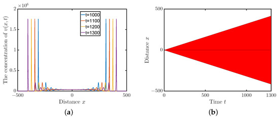
Figure 1. Solutions of system (3). (a) Evolution of virus population. (b) Evolution of the virus spreading domain.

Next, we studied the influences of the diffusion ability d_v and the radius r of compact support on the minimal wave speed $c^{\ast }$. Figure 2 shows that $c^{\ast }$ increases as d_v or r increases (the parameter values are fixed to those in Figure 1 except for d_v or r). Hence, decreasing the diffusion ability or diffusion radius may postpone the spread of the virus.

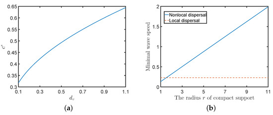
Figure 2. The influence of parameters on minimal wave speed. (a) The influence of diffusion ability on $c^{\ast }$ (nonlocal dispersal). (b) The influence of radius r of compact support.

Finally, we investigated the influences of the diffusion mode on the spreading speed. Assume that the virions can move either in the form of nonlocal dispersal or in the form of local dispersal (Laplace diffusion). Let the parameter values and initial data be the same as those in Figure 1 except for the radius r of compact support. Figure 3 shows that the solutions have a large hump for both local and nonlocal dispersals. It also shows that the virus with nonlocal dispersal spreads faster than the virus with local dispersal when the radius r is larger, while the inverse is true when the radius r is smaller. Thus, there may exist a threshold value $r^{\ast }$ such that a virus with nonlocal dispersal and a virus with local dispersal have the same asymptotic spreading speed when $r=r^{\ast }$ and a virus with nonlocal dispersal spreads faster (slower) than a virus with local dispersal when $r>r^{\ast }$ ($r<r^{\ast }$). Hence, nonlocal dispersal can postpone the spread of a virus when the diffusion radius is smaller and accelerate the spread of a virus when the diffusion radius is larger. In fact, it is found that the minimal wave speed for nonlocal dispersal is smaller than the minimal wave speed for local dispersal when the diffusion radius is small enough, and it can surpass the minimal wave speed for local dispersal when the radius increases (see Figure 2b), where the minimal wave speed for local dispersal can be defined by similar arguments to those in Section 2.

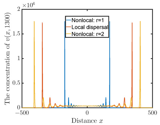
Figure 3. The concentration of $v(x,1300)$ for local or nonlocal operator.

4. Conclusions

Inspired by the phenomenon of viruses spreading like traveling waves [13], and considering the actual situation of virus transmission, we established a degenerate viral infection dynamical model with a nonlocal dispersal operator and analyzed the existence of traveling wave solutions of the model. We proved the existence of traveling wave solutions connecting the virus-free steady state and the positive steady state with wave speed $c\ge c^{\ast }$, as well as the nonexistence of traveling wave solutions with $0<c<c^{\ast }$. Thus, we can conclude that $c^{\ast }$ defined in Lemma 2 is the minimal wave speed of system (3). It is worth mentioning that the lower-bound estimation of the traveling wave solutions was achieved by adopting rescaling methods and the comparison principle, which is a challenge for some nonlocal models. While other methods may exist, our method is much simpler and can be easily adapted for application to other models with nonlocal dispersal.

Furthermore, the relationship between the minimal wave speed and the asymptotic spreading speed and the influences of the diffusion mode and diffusion ability on the minimal wave speed or the asymptotic spreading speed were investigated via simulations. Both the theoretical and numerical simulation results indicate the existence of traveling wave solutions of system (3), which is consistent with the evidence presented in [13]. Based on the simulations, we conclude that the asymptotic spreading speed may be larger than the minimal wave speed, and decreasing the diffusion ability or diffusion radius may postpone the spread of the virus. Nonlocal dispersal can postpone the spread of the virus when the diffusion radius is smaller and accelerate the spread when the diffusion radius is larger.

For the proposed model in this study, there is a typical characteristic, i.e., the target cell cannot move freely within the host, which is suitable for HBV or HCV infections. However, due to the diversity of viruses, there also exists some viruses, such as HIV or HTLV, for which their susceptible target cells and infected cells can move freely within the host and may have different mobilities. Therefore, if we consider nonlocal dispersal and different mobilities in both the target cells and virions, two interesting questions naturally arise that are worth further study: can the virions propagate as a traveling wave front, and what is its minimal wave speed? Moreover, during our analysis, we assumed that the kernel function $K(x)$ is symmetric. However, the actual environment is very complex, and the virions may diffuse asymmetrically within the host. The traveling wave solution and minimal wave speed of a model with an asymmetric dispersal kernel function should be further studied.

References

- World Health Organization. World health Statistics 2017: Monitoring health for the SDGs, Sustainable Development Goals; World Health Organization: Geneva, Switzerland, 2017. [Google Scholar]
- Jonit United Nations Programme on HIV/AIDS (UNAIDS). Miles to Go: Closing Gaps, Breaking Barriers, Righting Injustices; UNAIDS: Geneva, Switzerland, 2018. [Google Scholar]
- Perelson, A.; Neumann, A.; Markowitz, M.; Leonard, J.; Ho, D. HIV-1 dynamics in vivo: Virion clearance rate, infected cell life-span, and viral generation time. Science 1996, 271, 1582–1586. [Google Scholar] [CrossRef]
- Perelson, A.S.; Nelson, P.W. Mathematical analysis of HIV-1 dynamics in vivo. SIAM Rev. 1999, 41, 3–44. [Google Scholar] [CrossRef]
- Nowak, M.A.; May, R.M. Virus Dynamics: Mathematical Principles of Immunology and Virology; Oxford University Press: Oxford, UK, 2000. [Google Scholar]
- Korobeinikov, A. Global properties of basic virus dynamics models. Bull. Math. Biol. 2004, 66, 879–883. [Google Scholar] [CrossRef]
- Manna, K.; Chakrabarty, S.P. Chronic hepatitis B infection and HBV DNA-containing capsids: Modeling and analysis. Commun. Nonlinear Sci. Numer. Simul. 2015, 22, 383–395. [Google Scholar] [CrossRef]
- Shu, H.; Wang, L.; Watmough, J. Sustained and transient oscillations and chaos induced by delayed antiviral immune response in an immunosuppressive infection model. J. Math. Biol. 2014, 68, 477–503. [Google Scholar] [CrossRef]
- Song, X.; Neumann, A.U. Global stability and periodic solution of the viral dynamics. J. Math. Anal. Appl. 2007, 329, 281–297. [Google Scholar] [CrossRef]
- Xu, R.; Ma, Z. An HBV model with diffusion and time delay. J. Theor. Biol. 2009, 257, 499–509. [Google Scholar] [CrossRef] [PubMed]
- Murooka, T.T.; Deruaz, M.; Marangoni, F.; Vrbanac, V.D.; Seung, E.; von Andrian, U.H.; Tager, A.M.; Luster, A.D.; Mempel, T.R. HIV-infected T cells are migratory vehicles for viral dissemination. Nature 2012, 490, 283–287. [Google Scholar] [CrossRef]
- Fackler, O.T.; Murooka, T.T.; Imle, A.; Mempel, T.R. Adding new dimensions: Towards an integrative understanding of HIV-1 spread. Nat. Rev. Microbiol. 2014, 12, 563–574. [Google Scholar] [CrossRef] [PubMed]
- Strain, M.C.; Richman, D.D.; Wong, J.K.; Levine, H. Spatiotemporal dynamics of HIV propagation. J. Theor. Biol. 2002, 218, 85–96. [Google Scholar] [CrossRef] [PubMed]
- Wang, K.; Wang, W. Propagation of HBV with spatial dependence. Math. Biosci. 2007, 210, 78–95. [Google Scholar] [CrossRef] [PubMed]
- Lai, X.; Zou, X. Repulsion effect on superinfecting virions by infected cells. Bull. Math. Biol. 2014, 76, 2806–2833. [Google Scholar] [CrossRef] [PubMed]
- Murray, J.D. Mathematical biology: Spatial models and biomedical applications II. In Interdisciplinary Applied Mathematics, 3rd ed.; Springer: New York, NY, USA, 2003; Volume 18. [Google Scholar]
- Wang, J.B.; Li, W.T.; Sun, J.W. Global dynamics and spreading speeds for a partially degenerate system with non-local dispersal in periodic habitats. Proc. R. Soc. Edinb. Sect. 2018, 148, 849–880. [Google Scholar] [CrossRef]
- Zhao, G.; Ruan, S. Spatial and temporal dynamics of a nonlocal viral infection model. SIAM J. Appl. Math. 2018, 78, 1954–1980. [Google Scholar] [CrossRef]
- Bocharov, G.; Meyerhans, A.; Bessonov, N.; Trofimchuk, S.; Volpert, V. Spatiotemporal dynamics of virus infection spreading in tissues. PLoS ONE 2016, 11, e0168576. [Google Scholar] [CrossRef]
- Ren, X.; Tian, Y.; Liu, L.; Liu, X. A reaction-diffusion within-host HIV model with cell-to-cell transmission. J. Math. Biol. 2018, 76, 1831–1872. [Google Scholar] [CrossRef]
- Wang, W.; Ma, W.; Lai, X. Repulsion effect on superinfecting virions by infected cells for virus infection dynamic model with absorption effect and chemotaxis. Nonlinear Anal. Real World Appl. 2017, 33, 253–283. [Google Scholar] [CrossRef]
- Wang, W.; Ma, W. Travelling wave solutions for a nonlocal dispersal HIV infection dynamical model. J. Math. Anal. Appl. 2018, 457, 868–889. [Google Scholar] [CrossRef]
- Yang, Y.; Hsu, C.H.; Zou, L.; Zhou, J. A note on the propagation dynamics in a nonlocal dispersal HIV infection model. Proc. Am. Math. Soc. 2022, 150, 4867–4877. [Google Scholar] [CrossRef]
- Yang, F.Y.; Li, Y.; Li, W.T.; Wang, Z.C. Traveling waves in a nonlocal dispersal Kermack-McKendrick epidemic model. Discret. Contin. Dyn. Syst. B 2013, 18, 1969–1993. [Google Scholar] [CrossRef]
- Zhu, C.C.; Li, W.T.; Yang, F.Y. Traveling waves in a nonlocal dispersal SIRH model with relapse. Comput. Math. Appl. 2017, 73, 1707–1723. [Google Scholar] [CrossRef]
- Ducrot, A.; Magal, P. Travelling wave solutions for an infection-age structured epidemic model with external supplies. Nonlinearity 2011, 24, 2891–2911. [Google Scholar] [CrossRef]
- Li, Y.; Li, W.T.; Yang, F.Y. Traveling waves for a nonlocal dispersal SIR model with delay and external supplies. Appl. Math. Comput. 2014, 247, 723–740. [Google Scholar] [CrossRef]
- Wu, C.; Yang, Y.; Zhao, Q.; Tian, Y.; Xu, Z. Epidemic waves of a spatial SIR model in combination with random dispersal and non-local dispersal. Appl. Math. Comput. 2017, 313, 122–143. [Google Scholar] [CrossRef]
- Zhang, R.; Liu, S. Traveling waves for SVIR epidemic model with nonlocal dispersal. Math. Biosci. Eng. 2019, 16, 1654–1682. [Google Scholar] [CrossRef] [PubMed]
- Zhang, L.; Li, W.T.; Wu, S.L. Multi-type entire solutions in a nonlocal dispersal epidemic model. J. Dynam. Differ. Equations 2016, 28, 189–224. [Google Scholar] [CrossRef]
- Wu, J.; Zou, X. Traveling wave fronts of reaction-diffusion systems with delay. J. Dynam. Differ. Equations 2001, 13, 651–687. [Google Scholar] [CrossRef]
- Hou, R.; Xu, W.B. The traveling wave solutions in a mixed-diffusion epidemic model. Fractal Fract. 2022, 6, 217. [Google Scholar] [CrossRef]
- D’Elia, M.; Gunzburger, M. The fractional Laplacian operator on bounded domains as a special case of the nonlocal diffusion operator. Comput. Math. Appl. 2013, 66, 1245–1260. [Google Scholar] [CrossRef]
- Defterli, O.; D’Elia, M.; Du, Q.; Gunzburger, M.; Lehoucq, R.; Meerschaert, M.M. Fractional diffusion on bounded domains. Fract. Calc. Appl. Anal. 2015, 18, 342–360. [Google Scholar] [CrossRef]
- Neubert, M.G.; Parker, I.M. Projecting rates of spread for invasive species. Risk Anal. 2004, 24, 817–831. [Google Scholar] [CrossRef] [PubMed]
- Dahari, H.; Lo, A.; Ribeiro, R.M.; Perelson, A.S. Modeling hepatitis C virus dynamics: Liver regeneration and critical drug efficacy. J. Theor. Biol. 2007, 247, 371–381. [Google Scholar] [CrossRef] [PubMed]
Disclaimer/Publisher’s Note: The statements, opinions and data contained in all publications are solely those of the individual author(s) and contributor(s) and not of MDPI and/or the editor(s). MDPI and/or the editor(s) disclaim responsibility for any injury to people or property resulting from any ideas, methods, instructions or products referred to in the content. |
© 2024 by the authors. Licensee MDPI, Basel, Switzerland. This article is an open access article distributed under the terms and conditions of the Creative Commons Attribution (CC BY) license (https://creativecommons.org/licenses/by/4.0/).