Article

A Bearing Fault Diagnosis Method under Small Sample Conditions Based on the Fractional Order Siamese Deep Residual Shrinkage Network

1
College of Railway Transportation, Hunan University of Technology, Zhuzhou 412007, China
2
Zhuzhou Times New Material Technology Co, Ltd., Zhuzhou 412007, China
3
CRRC Zhuzhou Institute Co., Ltd., Zhuzhou 412001, China
4
College of Mechanical and Vehicle Engineering, Hunan University, Changsha 410082, China
5
The State Key Laboratory of Heavy-Duty and Express High-Power Electric Locomotive, Zhuzhou 412001, China
*
Authors to whom correspondence should be addressed.
Fractal Fract. 2024, 8(3), 134; https://doi.org/10.3390/fractalfract8030134
Submission received: 18 December 2023 / Revised: 15 February 2024 / Accepted: 21 February 2024 / Published: 26 February 2024

Abstract

:
A bearing fault is one of the major causes of rotating machinery faults. However, in real industrial scenarios, the harsh and complex environment makes it very difficult to collect sufficient fault data. Due to this limitation, most of the current methods cannot accurately identify the fault type in cases with limited data, so timely maintenance cannot be conducted. In order to solve this problem, a bearing fault diagnosis method based on the fractional order Siamese deep residual shrinkage network (FO-SDRSN) is proposed in this paper. After data collection, all kinds of vibration data are first converted into two-dimensional time series feature maps, and these feature maps are divided into the same or different types of fault sample pairs. Then, a Siamese network based on the deep residual shrinkage network (DRSN) is used to extract the features of the fault sample pairs, and the fault type is determined according to the features. After that, the contrastive loss function and diagnostic loss function of the sample pairs are combined, and the network parameters are continuously optimized using the fractional order momentum gradient descent method to reduce the loss function. This improves the accuracy of fault diagnosis with a small sample training dataset. Finally, four small sample datasets are used to verify the effectiveness of the proposed method. The results show that the FO-SDRSN method is superior to other advanced methods in terms of training accuracy and stability under small sample conditions.

1. Introduction

In all fields of modern industry, rotating machinery plays an important role. If these machines fail, the productivity of relevant industries will be seriously affected. In addition, if such faults are not resolved in time, the reliability and security of the entire system will be reduced, bringing huge economic losses. It can be seen that the health monitoring of rotating machinery is essential. In rotating machinery, rolling bearings are the core component and are used to support the operation of rotating machinery; therefore, the fault diagnosis of rolling bearings is of great significance to ensure the normal and smooth operation of rotating machinery and the safe and efficient production of modern industry [1].
There are two main methods for bearing fault diagnosis: signal-based processing and a data-driven approach. Data-driven methods have made significant strides in fault diagnosis due to their powerful nonlinear self-learning [2,3] and intelligent fault diagnosis capabilities [4,5,6,7,8,9,10,11,12,13,14,15,16]. For example, convolutional neural networks (CNNs) [4,5,6,7], generative adversarial networks (GANs) [8,9,10,11], long short-term memory networks [12,13,14], and deep residual shrinkage networks (DRSNs) [15,16] have been widely adopted. Ren et al. [8] proposed a dynamically balanced domain adversarial network embedded with a physically interpretable novel frequency band attention module for feature extraction to mitigate noise interference. Fu et al. [9] proposed a method based on feature augmentation GANs and auxiliary classifiers to enhance its ability to capture features. Zhao et al. [16] proposed a DRSN, which can detect important features via an attention mechanism. Although these methods improve the accuracy of fault diagnosis to some extent by improving the ability to capture network features, they all require a large amount of training data to achieve accurate fault diagnosis. In the actual industrial operation and maintenance environment, many devices have stringent production requirements, resulting in slow fault occurrence. However, once the fault occurs, the consequences are extremely serious, so it is difficult to collect the most effective fault information. In this case, the main challenges facing bearing fault diagnosis in industrial operation and maintenance environments are as follows: Firstly, there are not enough existing training samples to accurately predict the bearing fault type. Secondly, limited training samples make the model become unstable and prone to overfitting.
In view of the above situation, conducting research on small sample fault diagnosis methods can not only achieve a more accurate identification of equipment fault states under limited training data, thus improving the industrial production efficiency, but also has great significance in alleviating the difficulty of acquiring fault signals and reducing the input of manpower and material resources. To address these challenges, various researchers have devised methods to improve the accuracy of diagnosis by learning fault features with limited training data. Specifically, these methods can be summarized as transfer learning [17,18,19], data enhancement [20,21,22], meta learning [23,24,25], and metric learning [26,27,28,29]. Some studies on small sample fault diagnosis have been published in the field of mechanical fault diagnosis. Zhang et al. [17] applied an intra-domain transfer learning strategy to fault diagnosis. Based on transfer learning, Dong et al. [19] applied the diagnostic knowledge learned from simulation data to real scenarios. Zhang et al. [20] proposed a self-supervised meta learning GAN, which determines the optimal initialization parameters of the model by training various data generation tasks so that new data can be generated using a small amount of training data. Lei et al. [23] proposed a new modal fault diagnosis method based on meta learning (ML) and neural architecture search (NAS). One meta learning intelligent fault diagnosis method was proposed by Ma based on the multi-scale dilated convolution and relation module [24]. Su et al. [25] proposed a new method, called data reconstruction hierarchical recurrent meta-learning (DRHRML), for bearing fault diagnosis using small samples under different working conditions. Cheng et al. [26] proposed the MAML-Triplet fault classification learning framework based on the combination of MAML and the triplet neural network, and the fault type of the unknown signal was judged by comparing the Euclidean distance of the feature vectors between different signals. Zhao et al. [27] proposed a small sample bearing fault diagnosis method based on an improved Siamese neural network (ISNN); this method added a classification branch to the standard Siamese network and replaced the common Euclidean distance measurement with the network measurement. Xing et al. [28] used a CNN as a subnetwork of the Siamese network to use the maximum average difference instead of the commonly used Euclidean distance to achieve data enhancement. Liu et al. [29] proposed a fault diagnosis method based on a multi-scale fusion attention CNN (MSFACNN) to improve the fault diagnostic accuracy of aero engine bearings using small samples. In addition, other studies [30,31] combined attention mechanisms to extract richer depth features under small sample conditions. The authors in [32] combined five different neural network structures for experiments, while those in [33] combined multiple regression and fuzzy neural networks for small sample prediction.
Although the above methods have improved the performance of small sample fault diagnosis to a certain extent, there are still many problems. For example, transfer learning methods are highly dependent on source domain data and cannot ensure that the distribution of the source domain data and target domain data is completely similar. Some operations of the data enhancement method may change the detailed characteristics of the fault samples, leading to performance degradation in the real data. In addition, the meta learning method is highly complex, and the related technology is not mature, so the application of this method is limited. The combination of multiple models causes the model to become too complex, and it is easy to overfit during training. Metric learning only uses a simple distance measurement as a training guide and can be used in the case of a small number of training samples by means of comparison. It is simple to calculate and easy to operate, but the accuracy is low.
The fractional order is a generalization of the concept of integral calculus to fractions, whose exponents can be any real number, including decimals or fractions. Fractional order calculus is an extension of integral order calculus, which can more accurately describe real systems and obtain more accurate results [34]. The introduction of fractional derivatives and integrals can better describe nonlinear changes and increase the freedom degree of mathematical models. This provides greater flexibility and adaptability, which improves its application in real problems. Therefore, fractional order systems based on fractional order calculus have been proven to have excellent performance in various industries, for example, in the fields of speech recognition [35], image processing [36,37], and automatic control [38,39,40].
Since metric learning is suitable for small sample data and is easy to implement, DRSN has good feature extraction capability, and fractional optimization can seek better solutions. Therefore, aiming to resolve the problem of the low accuracy and poor stability of bearing fault diagnosis under small sample training data conditions, this paper combines metric learning, DRSN, and fractional order and proposes the FO-SDRSN method to solve this problem, verifying it with a small sample of training data. The contributions of this paper are summarized as follows:
(1)
The one-dimensional vibration signals are converted into two-dimensional time series feature maps, which is convenient for the neural network model to extract the feature of the signal. The combination of the DRSN and Siamese network is conducive to improving the feature extraction ability of fault signals under small sample conditions.
(2)
In the parameter updating process of neural network backpropagation, momentum and fractional order calculus are applied to the gradient descent optimizer to make it converge to the optimal solution, thus improving the accuracy of fault diagnosis in the case of limited training data.
(3)
In order to simulate the limited data conditions in engineering applications, four sets of small sample training data were selected from the CWRU dataset to analyze and verify the FO-SDRSN method, which provides a possibility for its further application in bearing fault diagnosis with small sample data.
The rest of this paper is organized as follows: Section 2 presents the proposed method, FO-SDRSN, in detail. Section 3 describes the experiments and evaluations, including data acquisition. In Section 4, the performance of the FO-SDRSN methods under various fractional orders is discussed. Finally, according to the above experiments, the study is summarized, and conclusions are drawn.

2. Proposed Method

The framework of the FO-SDRSN method for bearing fault diagnosis under limited data conditions is shown in Figure 1. This method consists of three stages. In the first stage, the vibration data are collected using the field acquisition unit of the vibration state monitoring system. After the sampling length is standardized in the sliding window, the one-dimensional vibration signal is converted into a two-dimensional time series feature map, which is then combined into fault sample pairs of the same or different types.
In the second stage, feature extraction is carried out. The fault sample pairs obtained in the first stage are successively input into FO-SDRSN for feature extraction, and the output feature vector pairs are obtained. Then, the Euclidean distance between each pair of output vectors is calculated to obtain the contrastive loss. In the third stage, fault diagnosis is carried out according to the output characteristics, and the fault diagnosis loss is calculated according to the diagnosis result and the real fault type. The contrastive loss and fault diagnosis loss are combined, and the momentum fractional order is used to optimize the network parameters, leading to a continual reduction in the loss function. On this basis, the optimal model is obtained by repeated iteration and is tested on the testing set. According to the features extracted from the model, the most likely category is predicted as the fault diagnosis result. The modeling steps are shown in Figure 1.

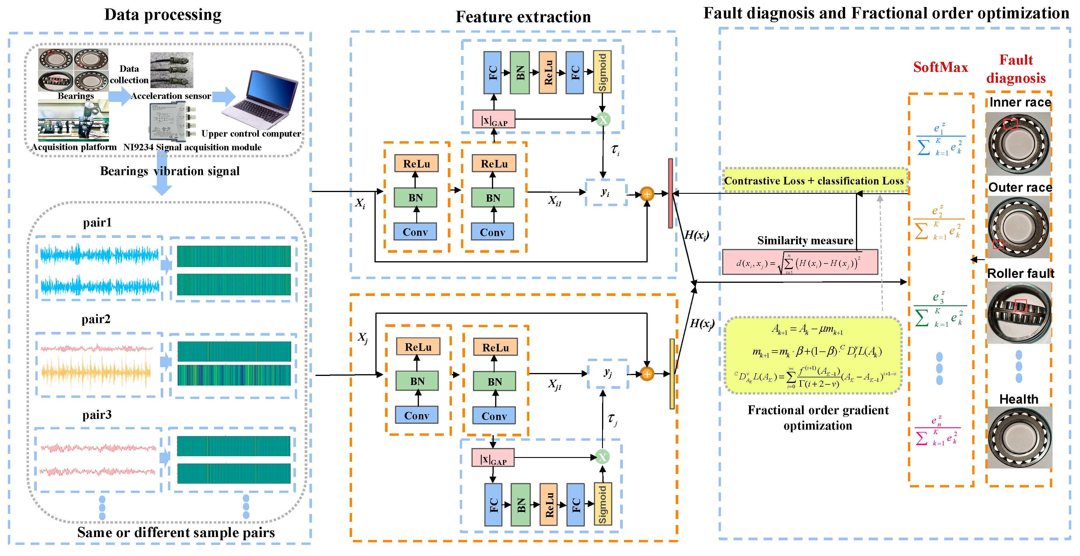
2.1. Data Processing and Feature Extraction

For the sample vibration data, a sliding window technique is used to sample a series of data samples, and the obtained samples are converted into two-dimensional time series feature maps. Then, the sample pairs of the same and different fault categories are obtained after pair processing. This pairing strategy can obtain richer information with a small amount of data, which lays a foundation for feature comparisons between samples of different categories and between samples of the same category during the feature extraction. Two feature vectors obtained from feature extraction are measured using Euclidean distance, with samples of the same category being labeled as similar and samples of different categories labeled as dissimilar. The samples are paired and labeled in data processing as follows:
( x i , x j , Y ) = P ( x i , x j )
The total number of training samples is N, each sample is represented by x, i and j both represent the index of the sample, and two samples are paired in turn. After pairing, there are C N 2 pairs of samples, and each sample pair can be represented by (xi, xj), where i, j = 1, 2…, N and ij. If xi and xj are fault sample pairs of the same type, Y = 1 is assigned; otherwise, Y = 0 is assigned, and p(⋅) denotes the labeling process for the sample pairs.
After the sample pairing is complete, all sample pairs are successively input into the FO-SDRSN for feature extraction. This process can be denoted as
F 1 = [ B N ( R e l u ( C o n v ( x , w ) ) ) ] n
where x refers to the input sample, w refers to the weight parameter of the FO-SDRSN, and Conv refers to the convolution operation. Relu refers to the activation function, which is used for the nonlinear transformation of neuronal output in the neural network. BN refers to Batch Normalization, which refers to the normalization of the input of each layer; ‘n’ denotes the repetition of the same operation ‘n’ times.
Sample xi is brought into F1 for feature extraction as follows:
x i 1 = F 1 ( x i , w ) 2
In the above formula, ‘2’ represents the execution of two F1 operations.
Following the feature extraction, the threshold value is determined through a contraction operation to minimize noise interference. The threshold determination process is outlined below:
F 2 = F C ( Re l u ( B N ( F C ( x , w ) ) ) )
Here, FC refers to the fully connected layer in a neural network.
α i = 1 1 + e F 2 ( a v e r a g e | x i 1 | )
Here, αi is the output after passing through the sigmoid.
τ i = α i a v e r a g e | x i 1 |
The above is the threshold calculation formula, and τ i is the calculated threshold value. In this network, the output of the residual module is shrunken using a shrinking operation to reduce the effect of noise. Here, the shrinking function is a soft-thresholding function. The shrinking operation can be expressed by
y i = { x i 1 τ i x i > τ i 0 τ i x L τ i x i 1 + τ i x i < τ i
Here, yi is the output after the threshold calculation.
After the feature extraction of sample xi using FO-SDRSN, it is expressed as follows:
H ( x i ) = x i + y i
where H ( x i ) is the output feature of xi after feature extraction from one side of the Siamese deep residual shrinkage network. Similarly, the output feature of xj after feature extraction from the other side of the Siamese Network can be defined as
H ( x j ) = x j + y j
The result of associating Equations (2)–(8) is as follows:
H ( x i ) = { x i + F 1 ( x i , w ) 1 1 + e F 2 ( a v e r a g e | x i 1 | ) a v e r a g e | F 1 ( x i , w ) | F 1 ( x i , w ) > 1 1 + e F 2 ( a v e r a g e | x i 1 | ) a v e r a g e | F 1 ( x i , w ) | x i 1 1 + e X L a v e r a g e | F 1 ( x i , w ) | F 1 ( x i , w ) F 1 ( x i , w ) 1 1 + e F 2 ( a v e r a g e | x i 1 | ) a v e r a g e | F 1 ( x i , w ) | x i + F 1 ( x i , w ) + 1 1 + e F 2 ( a v e r a g e | x i 1 | ) a v e r a g e | F 1 ( x i , w ) | F 1 ( x i , w ) < 1 1 + e F 2 ( a v e r a g e | x i 1 | ) a v e r a g e | F 1 ( x i , w ) |
The output feature vector of the FO-SDRSN method on both sides is measured using Euclidean distance, which is defined as
d ( x i , x j ) = i = 1 n ( H ( x i ) H ( x j ) ) 2
Here, H(xi) and H(xj) represent the fault features extracted from xi and xj, respectively, after applying the FO-SDRSN method. The value d is used to determine whether the input pair is of the same fault type: a smaller value of d indicates that the sample pair is similar, whereas larger values of d suggest that the sample pair is dissimilar. The contrastive loss function L1 is expressed as follows:
L 1 = 1 2 N n = 1 N Y d 2 + ( 1 Y ) max ( marg in   d , 0 ) 2
Here, N represents the number of samples, and Y indicates whether the input pair has the same type of fault. The expression Y = 1 signifies that the input pairs are similar, while Y = 0 indicates dissimilarity. The margin represents the threshold, with the default value set to 2.

2.2. Fault Diagnosis and Parameter Update

In order to achieve fault diagnosis, the extracted features H(xi) and H(xj) were fed to a SoftMax classifier. The output yn of the SoftMax classifier is defined by
y n = e H n ( x i ) n = 1 N class   e H n ( x i )
Here, n indicates the n-th class, yn is the predicted probability that the sample belongs to the n-th class, and Nclass is the number of categories, such that y n = 1 . In the above formula, Nclass = 10. After the probability of the sample belonging to 10 categories is predicted, respectively, the category with the largest prediction probability value is selected as the result of this fault diagnosis. The cross-entropy loss function is usually used as the objective function of multi-classification problems. In this paper, this function is the loss function of the fault diagnosis, which is expressed as
L 2 = n = 1 N class   t n log ( y n )
Here, tn indicates the actual fault type. When the sample belongs to the n-th class, tn = 1; otherwise, tn = 0. L1 and L2 are combined as total losses as follows:
L = L 1 + L 2 = 1 2 N n = 1 N Y d 2 + ( 1 Y ) max ( marg in   d , 0 ) 2 + n = 1 N class   t n log ( y n )
Then, when the loss function L is minimized, the momentum fractional step reduction algorithm is used to update and optimize the network parameters. Here, the Caputo fractional order method is adopted [41], which is denoted as
  C D t v L ( t ) = 1 Γ ( m v ) t 0 t f ( m ) ( τ ) ( t τ ) v m + 1 d τ
where v is the order of the fractional order, t is the parameter to be updated, m is the smallest integer greater than v, m − 1 < v < m, t0 is the initial value, and Γ ( α ) = 0 x α 1 e x d x is the Gamma function. The above formula can be derived as follows:
  C D t v L ( t ) = i = m f ( i ) ( t 0 ) Γ ( i + 1 v ) ( t t 0 ) i v
In order to ensure that the neural network converges to the real extreme point, the fault diagnostic accuracy fractional order is used in the parameter updating process of the neural network. In addition, to accelerate the convergence rate, a momentum term is added during the parameter updating process. The parameter updates are shown by
A k + 1 = A k μ m k + 1
where K is the number of iterations, A is the parameter to be updated, μ is the learning rate, and m is the momentum term. In order to accelerate the convergence rate, the momentum term is added when the parameter is updated. The momentum update rules are as follows:
m k + 1 = m k β + ( 1 β ) C D t v L ( A k )
β is the attenuation factor of momentum. When 0 < v < 1, m = 1, and substituting it into (17) yields the following:
  C D A K v L ( A K ) = i = 1 f ( i ) ( A K 1 ) Γ ( i + 1 v ) ( A K A K 1 ) i v
When 1 < v < 2, m = 2, and substituting it into (17) yields the following:
  C D A K v L ( A K ) = i = 2 f ( i ) ( A K 1 ) Γ ( i + 1 v ) ( A K A K 1 ) i v
The expression for 0 < v < 2 can be obtained by combining (20) and (21). The details are as follows:
  C D A K v L ( A K ) = i = 0 f ( i + 1 ) ( A K 1 ) Γ ( i + 2 v ) ( A K A K 1 ) i + 1 v
On that basis, the first term is kept, the absolute value is introduced, and the loss is calculated as follows:
  C D A K v L ( A K ) = f ( 1 ) ( A K 1 ) Γ ( 2 v ) | A K A K 1 + σ | 1 v
where δ is a small positive number to avoid the situation where the denominator is zero, so δ = 1 × 10⁻⁸.
By combining (19) and (23), the momentum update rule is obtained as follows:
m k + 1 = m k β + ( 1 β ) f ( 1 ) ( A K 1 ) Γ ( 2 v ) | A K A K 1 + σ | 1 v
By combining (18) and (24), the final update formula of the parameters in the FO-SDRSN method can be obtained as follows:
A k + 1 = A k μ ( m k β + ( 1 β ) f ( 1 ) ( A K 1 ) Γ ( 2 v ) ( | A K A K 1 | + δ ) 1 v )
In a nutshell, (1)–(13) among the above formulae represent the process of fault diagnosis by using the forward propagation of the FO-SDRSN method; (14) and (15) represent the process of calculating the loss according to the diagnosis results and the real fault type; and (18)–(25) represent the process of using the momentum fractional order part of the FO-SDRSN method to update the parameters so as to reduce losses and improve fault diagnostic accuracy. After the parameter update in (25) is completed, the above process is iterated to continuously reduce losses and improve the bearing fault diagnostic accuracy using small samples.

3. Experiments and Evaluations

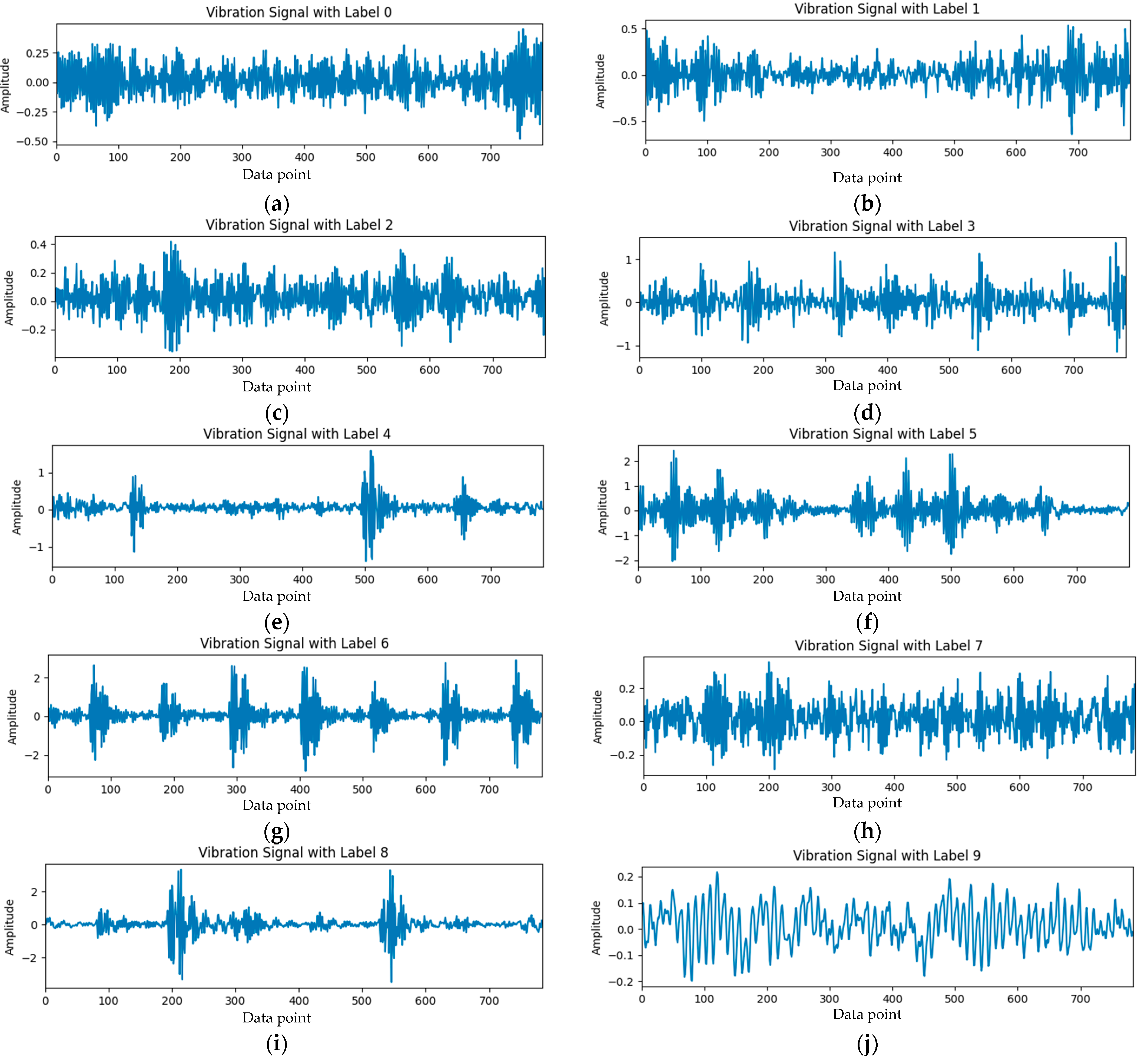
3.1. Data Acquisition

The steps for vibration data acquisition for bearing faults include selecting the vibration sensor, connecting and calibrating the sensor and mounting it on the bearings, and then selecting the sampling rate and connecting the sensor to the data acquisition device to record the vibration data under various fault and health conditions.
This study validates the proposed methodology using a bearings dataset sourced from Case Western Reserve University [42]. The bearings under consideration are of the SKF6205 type, and the fault states encompass roller fault, inner race fault, outer race fault, and health state. Each fault state comprises three crack diameters: 0.007 inch, 0.014 inch, and 0.021 inch. Consequently, the experiment encompasses nine types of fault data and one type of health status data, totaling ten different types of data.
Vibration signals from the bearings were captured using an acceleration sensor at a sampling frequency of 12 kHz. Following data acquisition, a sliding window with a length(s) of 784 and a step size of 1210 was applied for sampling. After this process, 300 samples were obtained for each fault state. In order to create small sample conditions, 10, 15, 20, and 30 of each type of signal were randomly selected and combined to form four small sample training sets. In addition, 20% of the samples from each fault type and health status were selected to build a testing set. Specific information regarding the experimental dataset is shown in Table 1. Figure 2a–j present the time-domain waveform graphs of signals corresponding to labels 0 to 9.
Converting the vibration signal into two-dimensional time series feature maps (as shown in Figure 3) can better retain the timing information of the original signal, and this conversion process is conducive to subsequent operations such as the convolution of the neural network model.

3.2. Experiments

In this section, the accuracy of the proposed method is evaluated using the four small sample datasets combined above and compared with other learning models, including the MSFACNN, CNN, DRSN, and Siamese–DRSN models. Each set of experiments was repeated five times to minimize unexpected errors.
During the training process, the training samples are randomly paired and input into the model. To evaluate the performance of various fault diagnosis methods under the conditions of limited training samples, box plots were employed to represent the accuracy and stability of the diagnosis results across five iterations for each model. Figure 4 illustrates the box plots for the fault diagnosis outcomes of five models across four datasets with small sample sizes. Figure 4a–d correspond to scenarios with 10, 15, 20, and 30 training samples for each fault type, respectively.
As seen in Figure 4a–d, under the four small sample datasets, the five test results under the FO-SDRSN method were distributed centrally, maintaining a high accuracy range. This shows that it maintains good stability and accuracy. However, the fault diagnostic accuracy of the CNN method is always lower than that of other improved methods. With the increasing amount of training data, the accuracy of diagnosis is not significantly improved. The average diagnostic accuracies of the FO-SDRSN method in the four small sample datasets is shown in Table 2, which are 82.61%, 91.46%, 92.69%, and 96.2%, respectively, and the standard deviations are 0.99, 0.6, 0.76, and 1.3, respectively. When there are 15 samples for each fault, the average accuracy of the fault diagnosis is 2.27% higher compared to the progressive Siamese–DRSN method. Compared with other advanced methods, it is further shown that the FO-SDRSN method has higher fault diagnostic accuracy and good stability under small sample conditions.
Figure 5 shows the test accuracy curve of each model with epoch change under the four small sample datasets. After conducting five experiments and excluding outliers, we selected the accuracy curves corresponding to the minimum loss functions for plotting. In Figure 5a–d, it can be observed that with an increase in the number of training samples, the convergence speed of each model improves. Additionally, the CNN model demonstrates a faster convergence speed, but with the lowest fault diagnostic accuracy, while the DRSN model exhibits the slowest convergence speed and the FO-SDRSN method shows a moderate convergence speed.
In order to explore the diagnostic effects of various models on each kind of fault, when the number of training samples for each type of fault was 15, a confusion matrix (Figure 6) was used to describe them.
In this figure, the ordinate indicates the real label value, and the abscissa indicates the predicted label value. The higher the coincidence between the predicted label value and the real label value, the better the diagnostic effect of this type of fault. In Figure 6a–f, each subfigure represents the confusion matrix under the SVM model, CNN model, MSFACNN model, DRSN model, Siamese–DRSN model, and FO-SDRSN model, respectively, when the number of training samples for each type of fault is 15. As can be seen in Figure 6a, the diagnostic effect of the SVM model based on machine learning on 10 kinds of faults is much lower than that of the other neural network models. Figure 6b–e reveal a substantial number of fault diagnosis errors for faults labeled 0, 1, and 2 in the respective models, indicating poor diagnostic efficacy. Compared with the other five methods, the FO-SDRSN method illustrated in Figure 6f demonstrates greater effectiveness in diagnosing various fault types (labeled 3–9). Notably, it performs better in diagnosing faults labeled 0, 1, and 2, which pose challenges for the other five models. The correct diagnosis rates for these three faults are 52/60, 42/60, and 47/60, respectively.
In order to more intuitively understand the excellent feature extraction capability of FO-SDRSN, when the number of training samples for each fault type is 15, t-SNE technology is used to visualize the feature extraction results in a two-dimensional space. Different colors represent different fault types. As depicted in Figure 7, the higher the clustering degree of the same color block distribution, the lower the clustering degree with other color blocks, indicating that the model has a better feature extraction effect on such faults.
Figure 7a illustrates the distribution of various fault data before the experiment. It can be observed that before the experiment, all fault types were mixed and difficult to distinguish individually. Figure 7b–e show two-dimensional representations of feature extraction results using the CNN, MSFACNN, DRSN, and Siamese–DRSN methods under small sample conditions. From the traditional CNN in Figure 7b to the FO-SDRSN method in Figure 7f, we can clearly see that different types of fault features gradually show a better clustering effect, indicating that the feature extraction capability of each model from CNN to FO-SDRSN is gradually enhanced. The remarkable feature extraction capability of the FO-SDRSN method facilitates the model in distinguishing between different fault types during fault diagnosis.

4. Discussion

In order to further investigate the optimal characteristics of the FO-SDRSN method, the diagnostic effectiveness of the FO-SDRSN method under different order conditions was explored on the above four types of small sample datasets. Figure 8a–d, respectively, show the average fault diagnostic accuracy of different fractional orders on four small sample datasets with 10, 15, 20, and 30 training samples for each type of fault. The abscissa indicates the change in the gradient update order v from 0.1 to 1.9, where v increases in steps of 0.1. The ordinate indicates the average diagnostic accuracy of the testing data.
As shown in Figure 8a, when the number of training samples for each type of fault is 10, the average fault diagnostic accuracy is higher for the fractional orders equal to 1.1 and 1.8 in the testing set. Similarly, Figure 8b reveals that with 15 training samples for each fault, the fractional orders equal to 1.1 and 1.5 exhibit higher average fault diagnostic accuracy. In Figure 8c, for 20 training samples per fault type, the fractional orders equal to 1.2, 1.6, and 1.7 demonstrate higher average fault diagnostic accuracy. Finally, as illustrated in Figure 8d, when there are 30 training samples for each fault, the fractional orders equal to 0.4, 1.2, and 1.6 can yield relatively higher average fault diagnostic accuracy.
Overall, under these four types of small sample datasets, the fault diagnosis performance of each fractional order less than 1.0 is inferior to that between orders of 1.1 and 1.9. However, when the fractional order is greater than or equal to 1.1, no significant change is observed in the diagnostic performance. When the sample number of various faults is small and the fractional order is equal to 1.1, the fault diagnostic effect is better. With the increase in the sample size of each type of fault, the fault diagnostic effect is better when the fractional orders are equal to 1.2 and 1.6.
Figure 9a–d show the accuracy distribution box plot of five fault diagnoses on four small sample datasets under various fractional orders. The abscissa indicates the change in the gradient update order v from 0.1 to 1.9, where v increases in increments of 0.1. The ordinate indicates the test accuracy.
As can be seen from Figure 9a, when the number of training samples for each fault type is 10, the fault diagnostic accuracy distribution is more concentrated and stable for fractional orders equal to 0.3, 1.1, 1.4, and 1.6. In Figure 9b, when the number of training samples for each fault type is 15, the fault diagnostic accuracy distribution is more concentrated and stable for fractional orders equal to 0.3, 1.1, 1.5, and 1.8. In Figure 9c, when the number of training samples for each fault type is 20, the fault diagnostic accuracy distribution is more concentrated and stable for fractional orders equal to 1.2, 1.6, 1.7, and 1.8. In Figure 9d, when the number of training samples for each fault type is 30, the fault diagnostic accuracy distribution is more concentrated and stable for fractional orders equal to 1.1, 1.2, 1.6, 1.7, and 1.8.
In summary, the stability of fractional orders ranging from 0.1 to 0.9 is lower compared to that of fractional orders ranging from 1.1 to 1.9. Moreover, when the number of samples is small, the stability of order 1.1 is notably higher. As the number of samples increases, the stability of the fractional orders equal to 1.2, 1.6, and 1.7 is better.
Figure 10a–d show the test accuracy curve of the FO-SDRSN method across four small sample datasets, illustrating how they change with epochs under different fractional orders. The above order with better accuracy and stability (1.1, 1.2, 1.6, 1.7) is selected for comparison. In the figure, the abscissa indicates the epoch, and the ordinate indicates the test accuracy. Different orders are represented by solid lines of different colors. By comparing the performance distribution of the model on the four small sample datasets, it can be concluded that with the increase in the training data, the convergence rate of each fractional order of the FO-SDRSN method is gradually accelerated.
As can be seen from Figure 10a, the fractional orders equal to 1.1 and 1.2 exhibit stable convergence within 150 epochs of training on this small sample dataset. Figure 10b reveals that all orders demonstrate stable convergence. From Figure 10c, it can be observed that within the first 150 epochs of training on this small sample dataset, all orders converge stably except for order 1.7. Figure 10d highlights that the fractional orders of 1.2 and 1.6 have stably converged within 150 epochs of training. These findings indicate that the fractional orders of 1.1 and 1.2 consistently achieve stable convergence under the four small sample datasets.
Through a comprehensive analysis of the average prediction accuracy, stability in multiple tests, and stability in single convergence, it is observed that, in scenarios with a limited sample size—specifically when the number of training samples for each fault type is below or equal to 15—the effect of the FO-SDRSN method is better when the fractional orders are equal to 1.1. As the training sample size expands, when the number of training samples for each fault type is between 15 and 30, the effect of the FO-SDRSN method is better when the fractional orders are equal to 1.2. Thus, the fault diagnosis performance of the FO-SDRSN method under different orders is related to the amount of small sample data.

5. Conclusions

In this paper, a small sample bearing fault diagnosis method based on FO-SDRSN was proposed to solve the problem of bearing fault diagnosis under limited data constraints. After obtaining the vibration data from the bearing faults, the input vibration data were sampled with a sliding window. Then, these data were converted into two-dimensional time series feature maps, which were divided into fault sample pairs of the same or different types. Subsequently, the Siamese deep residual shrinkage network based on momentum fractional order was used to diagnose the bearing fault. Finally, the effectiveness of the proposed method was evaluated and verified using four small sample datasets with different amounts of training data, and the effect of bearing fault diagnosis under different fractional orders was discussed. The conclusions are as follows:
(1)
The FO-SDRSN method can be used to diagnose bearing fault types under small sample conditions. This method can further reduce the loss during the repeated iterative updating of the network parameters, and the results are constantly close to the optimal solution, thus improving the accuracy of bearing fault diagnosis under small sample conditions.
(2)
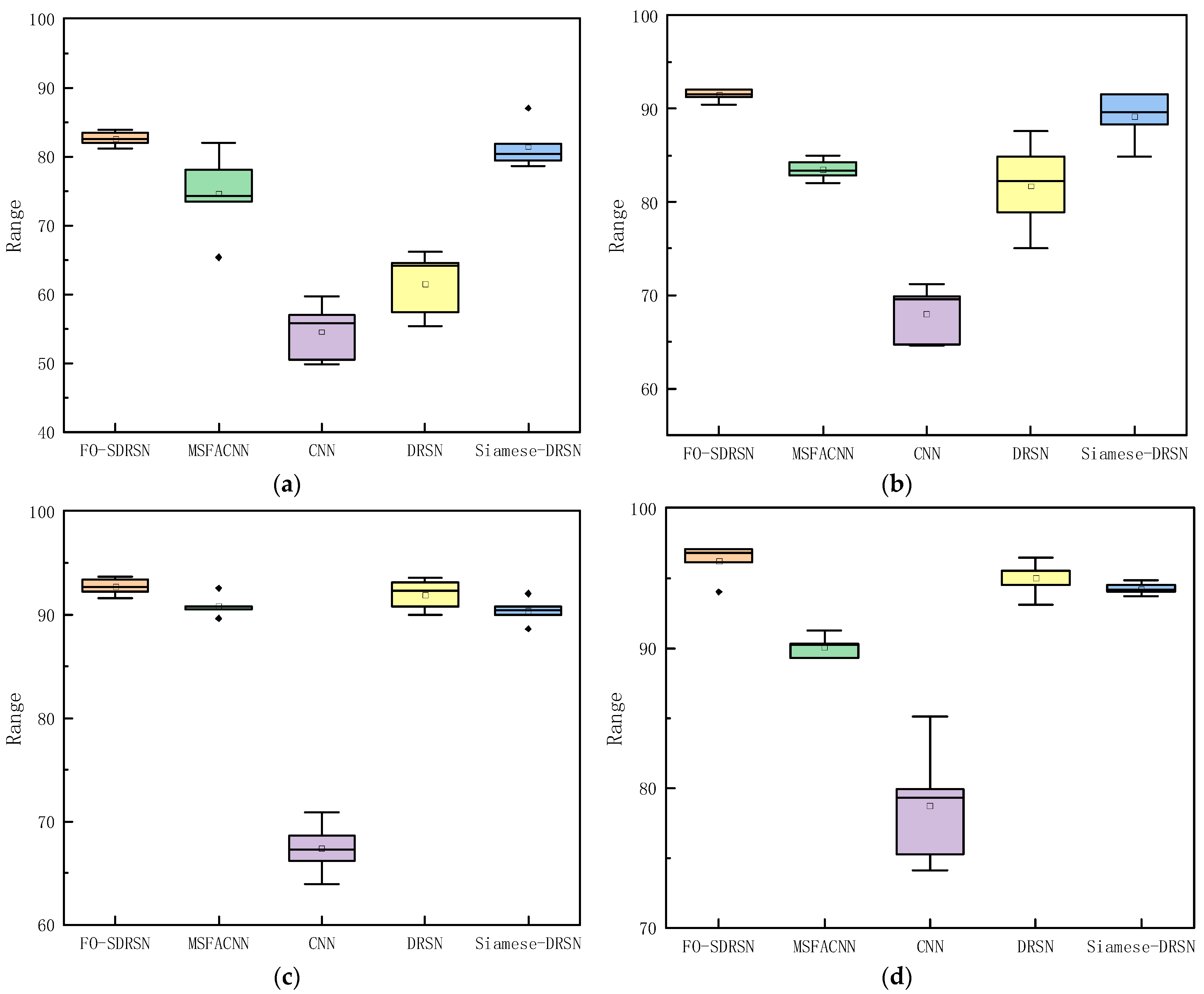
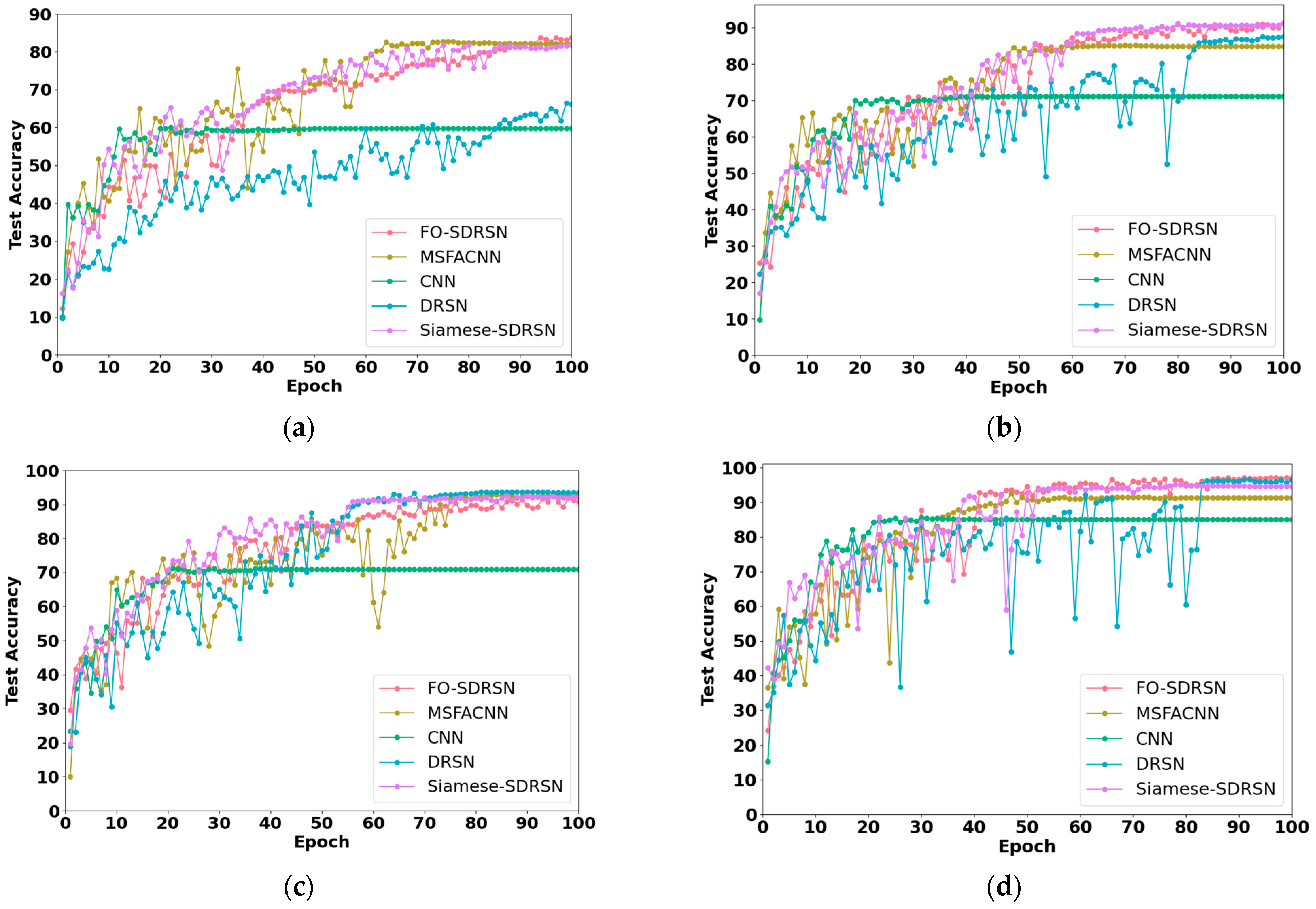
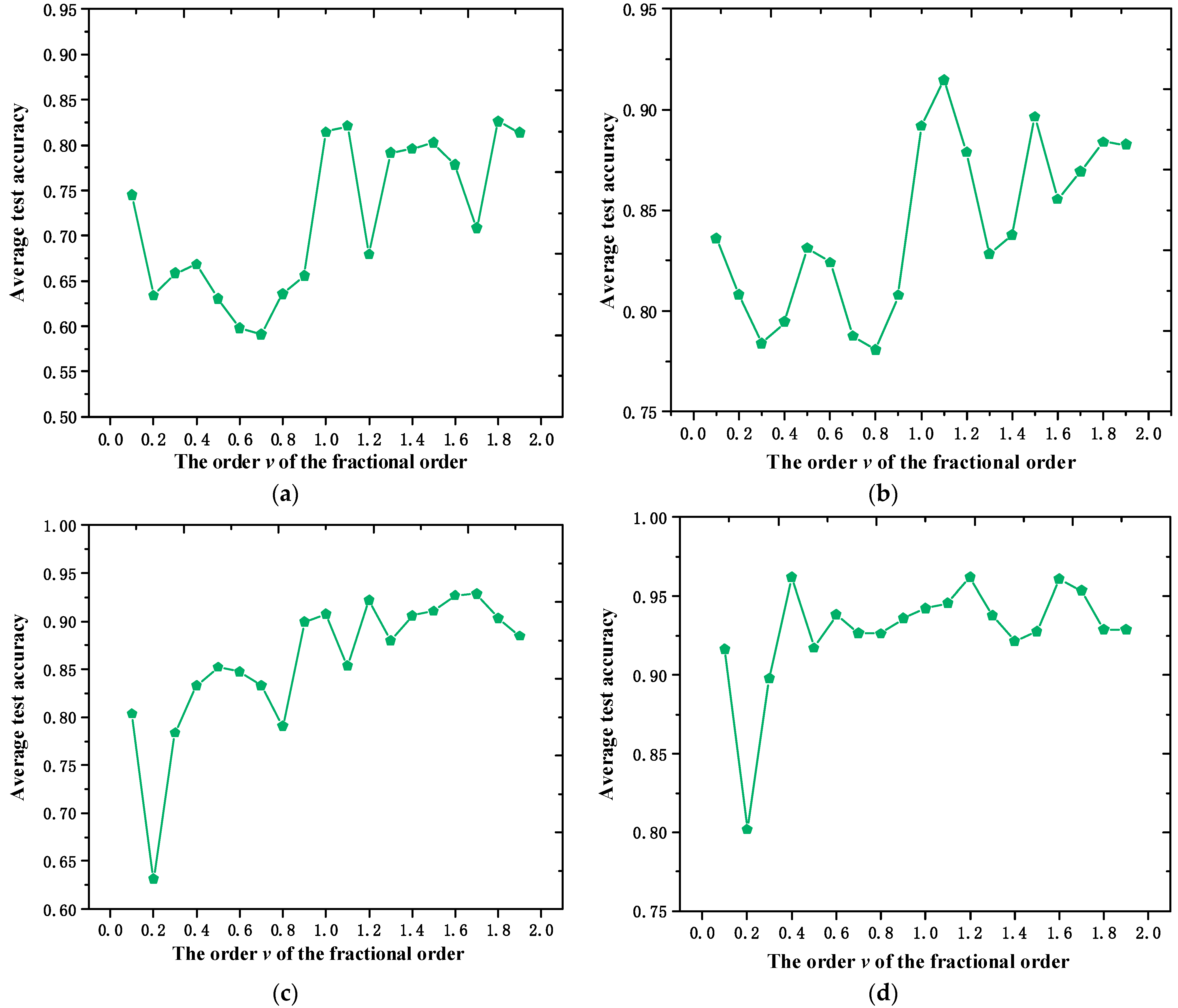
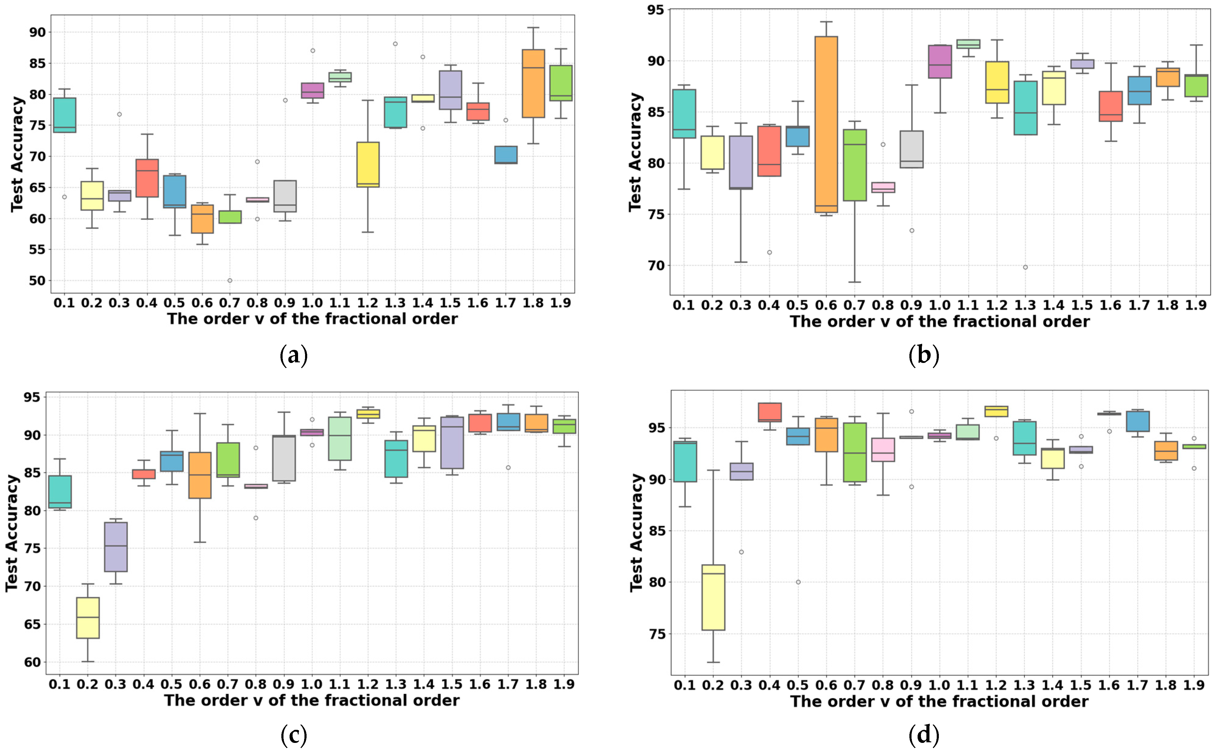
The experiments indicated that the FO-SDRSN method was more accurate and stable than other progressive methods under the given four small sample datasets. When the number of samples for each fault was 15, the average fault diagnostic accuracy was 2.27% higher than that of the progressive Siamese–DRSN method. The Discussion Section shows that the fault diagnosis performance of the FO-SDRSN method under different orders was associated with the quantity of small sample data.
(3)
In cases where there are limited data, the improvement in the accuracy of bearing fault diagnosis is crucial for the subsequent rapid and targeted maintenance and enhancement of the working efficiency of rotating machinery. The improvements demonstrated in this study also provide a new approach for the fault diagnosis of bearings equipment under actual industrial operation and maintenance conditions. This study was validated with publicly available datasets, so the robustness and applicability of the proposed method will be further verified in different engineering scenarios.

Author Contributions

Conceptualization, T.L. and X.W.; methodology, T.L. and X.W.; validation, T.L., X.W., and C.H.; formal analysis, T.L. and Z.L.; investigation, X.W.; resources, C.H.; data curation, T.L., X.W., and Y.C.; writing—original draft preparation, T.L. and X.W.; writing—review and editing, X.W.; supervision, R.D., J.Y., and C.Z.; project administration, T.L. and J.Y.; funding acquisition, C.Z. and J.Y. All authors have read and agreed to the published version of the manuscript.

Funding

This research was funded by the National Natural Science Foundation of China (Nos. 62373142, 62173137, and 52172403) and the State Key Laboratory of Heavy-duty and Express High-power Electric Locomotive.

Institutional Review Board Statement

Not applicable.

Informed Consent Statement

Not applicable.

Data Availability Statement

The data presented in this study are available upon request from the corresponding author.

Conflicts of Interest

Authors Tao Li, Xiaoting Wu, Zhuhui Luo, Caichun He and Jun Yang were employed by the company Zhuzhou Times New Material Technology Co, Ltd. Author Yanan Chen was employed by the company CRRC Zhuzhou Institute Co., Ltd. The remaining authors declare that the research was conducted in the absence of any commercial or financial relationships that could be construed as a potential conflict of interest.

References

  1. Niu, G.; Liu, E.; Wang, X.; Ziehl, P.; Zhang, B. Enhanced Discriminate Feature Learning Deep Residual CNN for Multitask Bearing Fault Diagnosis with Information Fusion. IEEE Trans. Ind. Inform. 2022, 19, 762–770. [Google Scholar] [CrossRef]
  2. Liu, K.; Yang, P.; Wang, R.; Jiao, L.; Li, T.; Zhang, J. Observer-Based Adaptive Fuzzy Finite-Time Attitude Control for Quadrotor UAVs. IEEE Trans. Aerosp. Electron. Syst. 2023, 59, 8637–8654. [Google Scholar] [CrossRef]
  3. Liu, K.; Yang, P.; Jiao, L.; Wang, R.; Yuan, Z.; Dong, S. Antisaturation fixed-time attitude tracking control based low-computation learning for uncertain quadrotor UAVs with external disturbances. Aerosp. Sci. Technol. 2023, 142, 108668. [Google Scholar] [CrossRef]
  4. Huang, D.; Zhang, W.-A.; Guo, F.; Liu, W.; Shi, X. Wavelet Packet Decomposition-Based Multiscale CNN for Fault Diagnosis of Wind Turbine Gearbox. IEEE Trans. Cybern. 2021, 53, 443–453. [Google Scholar] [CrossRef] [PubMed]
  5. Li, C.; Chen, J.; Yang, C.; Yang, J.; Liu, Z.; Davari, P. Convolutional Neural Network-Based Transformer Fault Diagnosis Using Vibration Signals. Sensors 2023, 23, 4781. [Google Scholar] [CrossRef] [PubMed]
  6. Zhang, C.; Huang, Q.; Yang, K.; Zhang, C. Intelligent Fault Diagnosis Method through ACCC-Based Improved Convolutional Neural Network. Actuators 2023, 12, 154. [Google Scholar] [CrossRef]
  7. Chen, J.; Huang, R.; Zhao, K.; Wang, W.; Liu, L.; Li, W. Multiscale Convolutional Neural Network With Feature Alignment for Bearing Fault Diagnosis. IEEE Trans. Instrum. Meas. 2021, 70, 3077673. [Google Scholar] [CrossRef]
  8. Ren, H.; Wang, J.; Dai, J.; Zhu, Z.; Liu, J. Dynamic Balanced Domain-Adversarial Networks for Cross-Domain Fault Diagnosis of Train Bearings. IEEE Trans. Instrum. Meas. 2022, 71, 3179468. [Google Scholar] [CrossRef]
  9. Fu, W.; Jiang, X.; Tan, C.; Li, B.; Chen, B. Rolling Bearing Fault Diagnosis in Limited Data Scenarios Using Feature Enhanced Generative Adversarial Networks. IEEE Sens. J. 2022, 22, 8749–8759. [Google Scholar] [CrossRef]
  10. Pham, M.T.; Kim, J.-M.; Kim, C.H. Rolling Bearing Fault Diagnosis Based on Improved GAN and 2-D Representation of Acoustic Emission Signals. IEEE Access 2022, 10, 78056–78069. [Google Scholar] [CrossRef]
  11. Yang, J.; Liu, J.; Xie, J.; Wang, C.; Ding, T. Conditional GAN and 2-D CNN for bearing fault diagnosis with small samples. IEEE Trans. Instrum. Meas. 2021, 70, 3119135. [Google Scholar] [CrossRef]
  12. Shi, J.; Peng, D.; Peng, Z.; Zhang, Z.; Goebel, K.; Wu, D. Planetary gearbox fault diagnosis using bidirectional-convolutional LSTM networks. Mech. Syst. Signal Process. 2022, 162, 107996. [Google Scholar] [CrossRef]
  13. Yang, M.; Liu, W.; Zhang, W.; Wang, M.; Fang, X. Bearing Vibration Signal Fault Diagnosis Based on LSTM-Cascade Cat-Boost. J. Internet Technol. 2022, 23, 1155–1161. [Google Scholar] [CrossRef]
  14. Aljemely, A.H.; Xuan, J.; Al-Azzawi, O.; Jawad, F.K.J. Intelligent fault diagnosis of rolling bearings based on LSTM with large margin nearest neighbor algorithm. Neural Comput. Appl. 2022, 34, 19401–19421. [Google Scholar] [CrossRef]
  15. Cao, X.; Xu, X.; Duan, Y.; Yang, X. Health Status Recognition of Rotating Machinery Based on Deep Residual Shrinkage Network Under Time-Varying Conditions. IEEE Sens. J. 2022, 22, 18332–18348. [Google Scholar] [CrossRef]
  16. Zhao, M.; Zhong, S.; Fu, X.; Tang, B.; Pecht, M. Deep Residual Shrinkage Networks for Fault Diagnosis. IEEE Trans. Ind. Inform. 2020, 16, 4681–4690. [Google Scholar] [CrossRef]
  17. Zhang, L.; Zhang, J.; Peng, Y.; Lin, J. Intra-Domain Transfer Learning for Fault Diagnosis with Small Samples. Appl. Sci. 2022, 12, 7032. [Google Scholar] [CrossRef]
  18. Zhou, X.; Li, A.; Han, G. An Intelligent Multi-Local Model Bearing Fault Diagnosis Method Using Small Sample Fusion. Sensors 2023, 23, 7567. [Google Scholar] [CrossRef] [PubMed]
  19. Dong, Y.; Li, Y.; Zheng, H.; Wang, R.; Xu, M. A new dynamic model and transfer learning based intelligent fault diagnosis framework for rolling element bearings race faults: Solving the small sample problem. ISA Trans. 2022, 121, 327–348. [Google Scholar] [CrossRef]
  20. Zhang, X.; Ma, R.; Li, M.; Li, X.; Yang, Z.; Yan, R.; Chen, X. Feature Enhancement Based on Regular Sparse Model for Planetary Gearbox Fault Diagnosis. IEEE Trans. Instrum. Meas. 2022, 71, 3176244. [Google Scholar] [CrossRef]
  21. Xie, Z.; Tan, X.; Yuan, X.; Yang, G.; Han, Y. Small Sample Signal Modulation Recognition Algorithm Based on Support Vector Machine Enhanced by Generative Adversarial Networks Generated Data. J. Electron. Inf. Technol. 2023, 45, 2071–2080. [Google Scholar] [CrossRef]
  22. Yang, X.; Liu, B.; Xiang, L.; Hu, A.; Xu, Y. A novel intelligent fault diagnosis method of rolling bearings with small samples. Measurement 2022, 203, 111899. [Google Scholar] [CrossRef]
  23. Lei, T.; Hu, J.; Riaz, S. An innovative approach based on meta-learning for real-time modal fault diagnosis with small sample learning. Front. Phys. 2023, 11, 1207381. [Google Scholar] [CrossRef]
  24. Ma, R.; Han, T.; Lei, W. Cross-domain meta learning fault diagnosis based on multi-scale dilated convolution and adaptive relation module. Knowl.-Based Syst. 2023, 261, 110175. [Google Scholar] [CrossRef]
  25. Su, H.; Xiang, L.; Hu, A.; Xu, Y.; Yang, X. A novel method based on meta-learning for bearing fault diagnosis with small sample learning under different working conditions. Mech. Syst. Signal Process. 2022, 169, 108765. [Google Scholar] [CrossRef]
  26. Cheng, Q.; He, Z.; Zhang, T.; Li, Y.; Liu, Z.; Zhang, Z. Bearing Fault Diagnosis Based on Small Sample Learning of Maml–Triplet. Appl. Sci. 2022, 12, 10723. [Google Scholar] [CrossRef]
  27. Zhao, X.; Ma, M.; Shao, F. Bearing fault diagnosis method based on improved Siamese neural network with small sample. J. Cloud Comput. 2022, 11, 79. [Google Scholar] [CrossRef]
  28. Xing, X.; Guo, W.; Wan, X. An Improved Multidimensional Distance Siamese Network for Bearing Fault Diagnosis with Few Labelled Data. In Proceedings of the 2021 Global Reliability and Prognostics and Health Management (PHM-Nanjing), Nanjing, China, 15–17 October 2021; pp. 1–6. [Google Scholar] [CrossRef]
  29. Liu, X.; Lu, J.; Li, Z. Multiscale Fusion Attention Convolutional Neural Network for Fault Diagnosis of Aero-Engine Rolling Bearing. IEEE Sens. J. 2023, 23, 19918–19934. [Google Scholar] [CrossRef]
  30. Liu, F.; Zhang, Z.; Chen, X.; Feng, Y.; Chen, J. A Novel Multisensor Orthogonal Attention Fusion Network for Multibolt Looseness State Recognition Under Small Sample. IEEE Trans. Instrum. Meas. 2022, 71, 3217855. [Google Scholar] [CrossRef]
  31. Xue, L.; Lei, C.; Jiao, M.; Shi, J.; Li, J. Rolling Bearing Fault Diagnosis Method Based on Self-Calibrated Coordinate Attention Mechanism and Multi-Scale Convolutional Neural Network Under Small Samples. IEEE Sens. J. 2023, 23, 10206–10214. [Google Scholar] [CrossRef]
  32. Gungor, O.; Rosing, T.; Aksanli, B. ENFES: ENsemble FEw-Shot Learning For Intelligent Fault Diagnosis with Limited Data. In Proceedings of the 2021 IEEE Sensors, Sydney, Australia, 31 October 2021–3 November 2021; pp. 1–4. [Google Scholar] [CrossRef]
  33. Li, T.; Wu, X.; He, Y.; Peng, X.; Yang, J.; Ding, R.; He, C. Small samples noise prediction of train electric traction system fan based on a multiple regression-fuzzy neural network. Eng. Appl. Artif. Intell. 2023, 126, 106781. [Google Scholar] [CrossRef]
  34. Zhao, C.; Dai, L.; Huang, Y. Fractional Order Sequential Minimal Optimization Classification Method. Fractal Fract. 2023, 7, 637. [Google Scholar] [CrossRef]
  35. Huang, L.; Shen, X. Research on Speech Emotion Recognition Based on the Fractional Fourier Transform. Electronics 2022, 11, 3393. [Google Scholar] [CrossRef]
  36. Yang, Q.; Chen, D.; Zhao, T.; Chen, Y. Fractional Calculus in Image Processing: A Review. Fract. Calc. Appl. Anal. 2016, 19, 1222–1249. [Google Scholar] [CrossRef]
  37. Henriques, M.; Valério, D.; Gordo, P.; Melicio, R. Fractional-Order Colour Image Processing. Mathematics 2021, 9, 457. [Google Scholar] [CrossRef]
  38. Yin, L.; Cao, X.; Chen, L. High-dimensional Multiple Fractional Order Controller for Automatic Generation Control and Automatic Voltage Regulation. Int. J. Control. Autom. Syst. 2022, 20, 3979–3995. [Google Scholar] [CrossRef]
  39. Marinangeli, L.; Alijani, F.; HosseinNia, S. A Fractional-order Positive Position Feedback Compensator for Active Vibration Control. IFAC-PapersOnLine 2017, 50, 12809–12816. [Google Scholar] [CrossRef]
  40. Li, T.; Wang, N.; He, Y.; Xiao, G.; Gui, W.; Feng, J. Noise Cancellation of a Train Electric Traction System Fan Based on a Fractional-Order Variable-Step-Size Active Noise Control Algorithm. IEEE Trans. Ind. Appl. 2023, 59, 2081–2090. [Google Scholar] [CrossRef]
  41. Sheng, D.; Wei, Y.; Chen, Y.; Wang, Y. Convolutional neural networks with fractional order gradient method. Neurocomputing 2020, 408, 42–50. [Google Scholar] [CrossRef]
  42. Loparo, K.A. Bearings Vibration Data Set Case Western Reserve University. [EB/OL]. Available online: http://www.eecs.cwru.edu/laborato-ry/bearing/download.htm (accessed on 1 September 2020).
Figure 1. FO-SDRSN method framework for fault diagnosis under small sample conditions.
Fractalfract 08 00134 g001
Figure 2. Time-domain waveform graphs of signals: (aj) represent signals corresponding to labels 0–9 respectively.
Fractalfract 08 00134 g002
Figure 3. Two-dimensional time characteristic sequence graphs of signals: (aj) represent signal corresponding to labels 0–9 respectively.
Fractalfract 08 00134 g003
Figure 4. Box plot of fault diagnostic accuracy distribution of different models under the four types of small sample datasets: (ad) represent small sample datasets with 10, 15, 20, and 30 training samples for each type of fault, respectively.
Fractalfract 08 00134 g004
Figure 5. Test accuracy curve of each model changes with epoch on four small sample datasets: (ad) represent small sample datasets with 10, 15, 20, and 30 training samples for each type, respectively.
Fractalfract 08 00134 g005
Figure 6. Confusion matrix for various models when the number of training samples of each type of fault is 15. (a) SVM model; (b) CNN model; (c) MSFACNN model; (d) DRSN model; (e) Siamese–DRSN model; (f) FO-SDRSN model.
Fractalfract 08 00134 g006
Figure 7. Feature visualization using various models when the number of training samples of each type of fault is 15. (a) Feature visualization of data distribution before fault diagnosis; (b) CNN model; (c) MSFACNN model; (d) DRSN model; (e) Siamese–DRSN model; (f) FO-SDRSN model.
Fractalfract 08 00134 g007
Figure 8. Average accuracy of different fractional orders on four small sample datasets: (ad) represent small sample datasets with 10, 15, 20, and 30 training samples for each type of fault, respectively.
Fractalfract 08 00134 g008
Figure 9. Box plot of 5 repeated experiments under different fractional orders on four small sample datasets: (ad) represent small sample datasets with 10, 15, 20, and 30 training samples for each type of fault, respectively.
Fractalfract 08 00134 g009
Figure 10. Precision curve of different fractional orders with epoch on four small sample datasets: (ad) represent small sample datasets with 10, 15, 20, and 30 training samples for each type of fault, respectively.
Fractalfract 08 00134 g010
Table 1. Experimental dataset.
LabelFault Size (Inch)Fault LocationNumber of Training Samples in Four Small Sample Datasets
00.007Roller10, 15, 20, 30
10.014Roller10, 15, 20, 30
20.021Roller10, 15, 20, 30
30.007Inner race10, 15, 20, 30
40.014Inner race10, 15, 20, 30
50.021Inner race10, 15, 20, 30
60.007Outer race10, 15, 20, 30
70.014Outer race10, 15, 20, 30
80.021Outer race10, 15, 20, 30
9-Health10, 15, 20, 30
Table 2. Experimental results using four small sample datasets.
ModelNumber of Training Samples for Each Type of Fault Is 10Number of Training Samples for Each Type of Fault Is 15Number of Training Samples for Each Type of Fault Is 20Number of Training Samples for Each Type of Fault Is 30
Average Accuracy (%)Standard DeviationAverage Accuracy (%)Standard DeviationAverage Accuracy (%)Standard DeviationAverage Accuracy (%)Standard Deviation
FO-SDRSN82.60910.98574691.461060.60393792.69480.76144296.201281.296661
MSFACNN74.627825.5389783.495141.03359690.841420.95234790.089760.724449
CNN54.563083.81464267.993522.78843867.378642.3305478.737863.899128
DRSN61.516124.30324881.709684.41898591.930341.348297951.145057
Siamese–DRSN81.428562.99443189.188322.46501890.357181.10866494.220760.392317
Disclaimer/Publisher’s Note: The statements, opinions and data contained in all publications are solely those of the individual author(s) and contributor(s) and not of MDPI and/or the editor(s). MDPI and/or the editor(s) disclaim responsibility for any injury to people or property resulting from any ideas, methods, instructions or products referred to in the content.

