Pattern Formation Mechanisms of Spatiotemporally Discrete Activator–Inhibitor Model with Self- and Cross-Diffusions

Abstract

In this paper, we aim to solve the issue of pattern formation mechanisms in a spatiotemporally discrete activator–inhibitor model that incorporates self- and cross-diffusions. We seek to identify the conditions that lead to the emergence of complex patterns and to elucidate the principles governing the dynamic behaviors that result in these patterns. We first construct a corresponding coupled map lattice (CML) model based on the continuous activator–inhibitor reaction–diffusion system. In the reaction stage, we examine the existence, uniqueness, and stability of the homogeneous stationary state and specify the parametric conditions for realizing these properties. Furthermore, by applying the center manifold theorem, we perform a flip bifurcation analysis and confirm that the model is capable of undergoing flip bifurcation. In the diffusion stage, we focus on the analysis of Turing bifurcation and determine the parameter conditions for the emergence of Turing instability. Through numerical simulations, we validate and explain the results of our theoretical analysis. Our study reveals various Turing instability mechanisms by coupling Turing and flip bifurcations, which include pure-self-diffusion-Turing instability, pure-cross-diffusion-Turing instability, flip-self-diffusion-Turing instability, flip-cross-diffusion-Turing instability, and chaos-self-diffusion-Turing instability mechanisms. Under different mechanisms, we illustrate the corresponding Turing patterns and discover a rich variety of pattern types such as labyrinthine, mosaic, alternating mosaic, colorful mottled grid patterns with winding and twisted bands, and patterns with dense patches and twisted bands nested together. Our research provides a theoretical framework and numerical support for understanding the complex dynamical behaviors and pattern formations in activator–inhibitor models with self- and cross-diffusions.

1. Introduction

The reaction–diffusion equations are some of the fundamental models used to describe the formation of spatiotemporal patterns [1]. The most common reaction–diffusion models are based on the following partial differential equations:

$$\left\{\begin{array}{c}{\displaystyle \frac{\partial u}{\partial t}=D_u{\nabla }^{2}u+f(u,v;ϵ)},\hfill \\ \\ {\displaystyle \frac{\partial v}{\partial t}=D_v{\nabla }^{2}v+g(u,v;ϵ)},\hfill \end{array}\right.$$

where u and v represent the densities of different chemicals, $D_u{\nabla }^{2}u$ and $D_v{\nabla }^{2}v$ describe the diffusion effects in space, $D_u$ and $D_v$ indicate the diffusion coefficients, $f(u,v;ϵ)$ and $g(u,v;ϵ)$ represent the reaction effects, and $ϵ$ indicates the parameters set. In 1952, Turing built on this reaction–diffusion theory to explain how, in the absence of genetic differences, biological forms can produce spatial patterns through chemical reactions and diffusion processes [2]. These spatial patterns are produced because of the unequal spatial diffusions. Therefore, this destabilization is called spatial-driven instability, and the resulting patterns are called Turing patterns. Turing’s pioneering works later opened up a whole new field of research. But initially, his seminal works did not attract much attention from scholars until 1972 when Gierer and Meinhardt became acquainted with Turing’s theory. In [3], Gierer and Meinhardt proposed several molecular models in the form of reaction–diffusion equations to explain the formation of a spatial pattern of tissue structures in embryology and regeneration, which include the depletion model, activator–inhibitor model with common sources, and activator–inhibitor model with different sources. They found that stationary patterns can emerge in certain chemical systems consisting of activators and inhibitors. Their findings exactly confirmed Turing’s theory. Thus, the 1970s marked the onset of an increasing fascination with Turing patterns, a trend that continues to this day [4].

Nowadays, Turing’s theory is widely used in many disciplines such as engineering [5,6,7], ethology [8,9], physics [10], ecology [11,12], and biology [13,14,15]. Recent studies that extend Turing’s theory generally branched out into many areas such as spatiotemporal complexity and novel patterns, impacts of stochasticity and noise on pattern formation [16], coupled map lattice model (CML model) [17,18], complex networks [19,20,21] and multiscale modeling [22], numerical simulations, and so on. The CML model is a type of discrete model widely used for studying the spatiotemporal dynamics of space and time discrete predator–prey systems [23,24]. Compared to the continuous models, the CML model has significant advantages in describing nonlinear characteristics and dynamic complexity. Firstly, the complex nonlinear characteristics, for example, fractals, frozen chaos, spatiotemporal intermittency, spatiotemporal chaos, defect turbulence, traveling wave, and so on, can be exhibited by the CML model [25,26]. Secondly, the CML model might display novel dynamical phenomena. For instance, Turing instability and Turing patterns can arise in the discrete competitive Lotka–Volterra model, which are not observed in the continuous version of the model [27]. Additionally, the CML model demonstrates the ability to capture discontinuous characteristics such as the patchy environment of fragmented habitats [23]. In comparison with other discrete models, the CML model also has some advantages. For example, the criteria for the emergence of patterns can be established theoretically, and the impact of parameter changes on pattern formation can be described quantitatively [23]. A CML model inherently represents a numerical algorithm, which means that numerical simulations conducted with a CML model typically exhibit high computational efficiency. The CML models are closely connected to the continuous spatiotemporal models, allowing for the application of several established theoretical results and methods for the analysis of the CML models [28,29].

Diffusion can lead to Turing instability. The current types of diffusion mainly include self-diffusion, cross-diffusion, convective diffusion, and fractional diffusion, among others. Cross-diffusion has been widely studied in the literature for its impact on reaction–diffusion systems [30,31], with these studies exploring how cross-diffusion influences pattern stability and spatial heterogeneity. However, existing research mainly focuses on classical reaction–diffusion models, whereas in our study, we combine cross-diffusion with the coupled map lattice (CML) method to investigate the profound effects of cross-diffusion on Turing instability and pattern formation. The CML methods have been widely employed in analyzing predator–prey systems, offering an effective framework for understanding spatiotemporal dynamics in discrete systems. The Gierer–Meinhardt model, as one of the most influential reaction–diffusion systems with activators and inhibitors, has attracted extensive attention. Some scholars’ research on these models primarily focuses on continuous models. The interaction between Hopf bifurcation and Turing bifurcation, where the instability phenomena are generally limited to pure Turing instability has been widely investigated [32,33,34,35,36]. In recent years, many scholars carried out bifurcation analysis on the Gierer–Meinhardt model with time delay terms [37,38,39,40]. In [41], the authors carried out Bogdanov–Takens bifurcation of codimension 3 in a Gierer–Meinhardt model. In [42], the authors proposed a method for analyzing the dynamic behavior of the Gierer–Meinhardt model in two-dimensional space by using the finite difference method, and they investigate the impact of the inhibitor degradation rate on pattern formation. In fact, there are also some scholars who have studied the pattern formation mechanism of the discrete Gierer–Meinhardt model. In [43], the authors investigate a semi-discrete Gierer–Meinhardt model and obtain the Turing instability conditions. In [44], the authors studied the dynamical behaviors and pattern formations of a CML model based on a Gierer–Meinhardt system with different sources. The diffusion terms are mainly about the self-diffusions. In [45], the authors investigated the spatiotemporal dynamics and Turing patterns of a spatially discrete depletion type Gierer–Meinhardt model with self-diffusion and cross-diffusion, and they simulated the evolution of pattern size and type as the cross-diffusion coefficient varies. In [46], the authors studied the bifurcation and pattern dynamics of a spatiotemporal discrete system with self-diffusion and numerically simulated the bifurcation behavior and patterns. More corresponding research and applications on the Gierer–Meinhardt systems can be seen in [47,48,49,50] and the references therein. Despite these efforts, research on pattern formation mechanisms driven by multiple bifurcations, such as the interplay between flip bifurcation and Turing instability, remains scarce in the context of spatially and temporally discrete activator–inhibitor systems, particularly when cross-diffusion terms are involved. This paper addresses this gap by developing a novel CML model based on an activator–inhibitor system, which incorporates both self- and cross-diffusions. Through this model, we aim to uncover new insights into spatiotemporal dynamics and provide a more comprehensive understanding of the mechanisms underlying pattern formation in spatiotemporal discrete systems.

The organization of this paper is as follows. In Section 2, we construct a CML model corresponding to the continuous activator–inhibitor system with self- and cross-diffusions in Section 2.1. For the CML model, we first study the existence and stability of the homogeneous stationary state in Section 2.2. In Section 3, we carry out a detailed analysis of flip bifurcation at the reaction stage in Section 3.1 and Turing bifurcation at the diffusion stage in Section 3.2. We obtain the existence conditions of flip bifurcation and Turing bifurcation. In Section 4, we perform the numerical simulations to explain the theoretical results. During the simulations, we show the patterns induced by different mechanisms. In Section 5, we give a brief discussion and conclusion. In Appendix A, we show a flowchart of our work.

2. The CML Model and Stability Analysis

In this section, we first use the CML method to discretize the continuous activator–inhibitor model with different sources to obtain the corresponding CML model. Then, we carry out the stability analysis for the homogeneous stationary state.

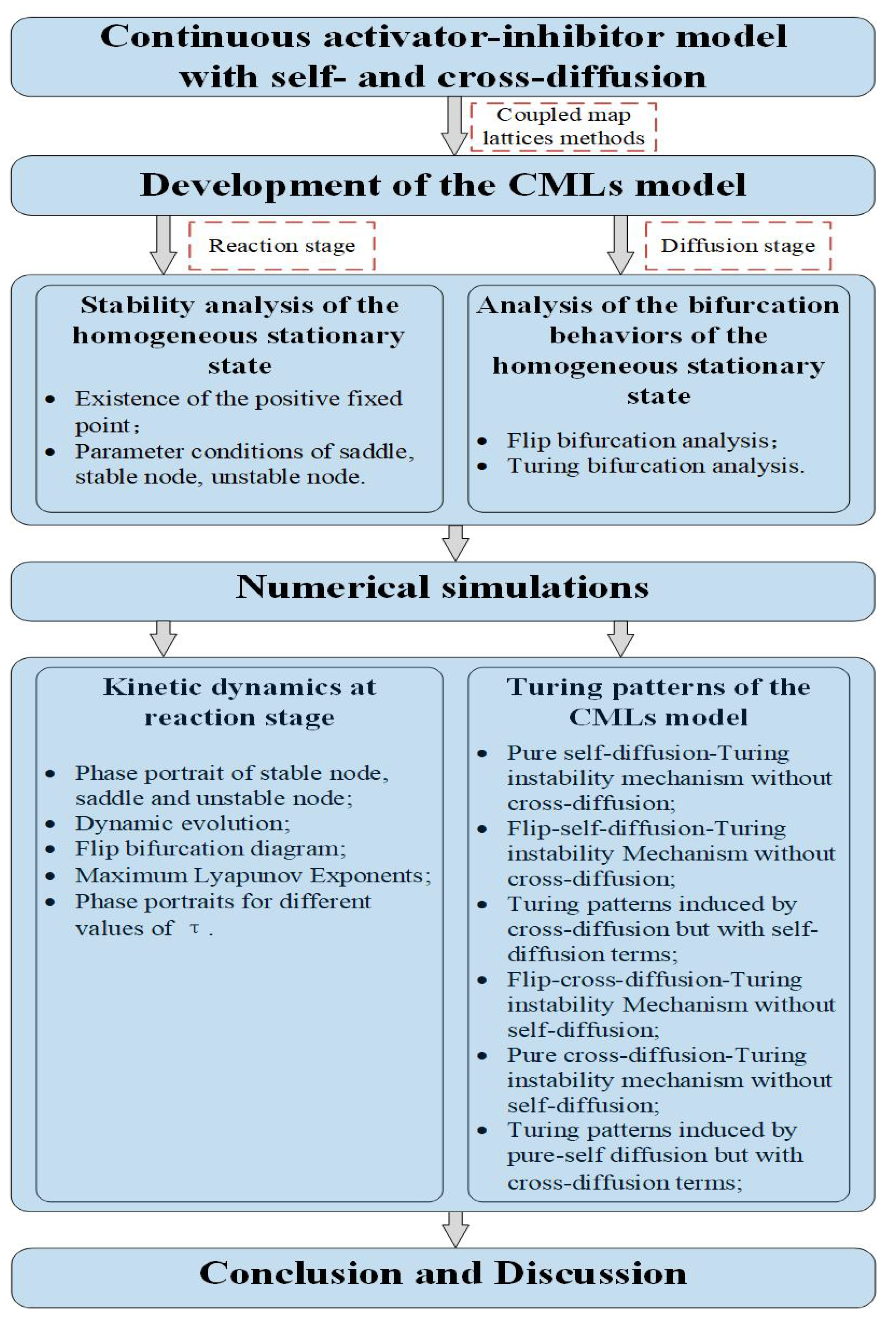
2.1. Development of CML Model

One of the continuous activator–inhibitor models in [3] in two-dimensional space with self- and cross-diffusions has the following form:

$$\left\{\begin{array}{c}{\displaystyle \frac{\partial a}{\partial t}={\rho }_0\rho +c\rho \frac{a^2}{h}-\mu a+D_{a1}(\frac{{\partial }^{2}a}{\partial x^2}+\frac{{\partial }^{2}a}{\partial y^2})+D_{a2}(\frac{{\partial }^{2}h}{\partial x^2}+\frac{{\partial }^{2}h}{\partial y^2})},\hfill \\ \\ {\displaystyle \frac{\partial h}{\partial t}=c^{\prime }{\rho }^{\prime }{a}^2-\nu h+D_{h1}(\frac{{\partial }^{2}a}{\partial x^2}+\frac{{\partial }^{2}a}{\partial y^2})+D_{h2}(\frac{{\partial }^{2}h}{\partial x^2}+\frac{{\partial }^{2}h}{\partial y^2})},\hfill \end{array}\right.$$

(1)

where $a(x,y,t)$ and $h(x,y,t)$ indicate the activator and inhibitor densities with positive self-diffusion constants $D_{a1}$ and $D_{h2}$ and cross-diffusion constants $D_{a2}$ and $D_{h1}$, respectively, at a spatial position $(x,y)$ at time $t>0$. The positive constants $\rho$ and ${\rho }^{\prime }$ indicate the distributions of sources of activators and inhibitors, respectively. The first-order kinetics $\mu a$ and $\nu h$ represent the consumption by any combination of enzyme degradation, leakage, and re-uptake by the sources. $\mu$, $\nu$, c and $c^{\prime }$ are positive constants. The activator has a basal production, which is proportional to $\rho$ with portion coefficient ${\rho }_0$.

By scaling, $a={\displaystyle \frac{c\rho }{c^{\prime }{\rho }^{\prime }}}A$, $h={\displaystyle \frac{c^2{\rho }^2}{c^{\prime }{\rho }^{\prime }\nu }}H$, $t={\displaystyle \frac{T}{\nu }}$, and letting $c_0={\displaystyle \frac{c^{\prime }{\rho }^{\prime }{\rho }_0}{c\nu }}$, $D_{A1}={\displaystyle \frac{D_{a1}}{\nu }}$, $D_{A2}={\displaystyle \frac{D_{a2}c\rho }{{\nu }^2}}$, $D_{H1}={\displaystyle \frac{D_{h1}}{c\rho }}$, $D_{H2}={\displaystyle \frac{D_{h2}}{\nu }}$, $\overline{\mu }={\displaystyle \frac{\mu }{\nu }}$, we can rewrite system (1) as follows:

$$\left\{\begin{array}{c}{\displaystyle \frac{\partial A}{\partial T}=c_0+\frac{A^2}{H}-\overline{\mu }A+D_{A1}(\frac{{\partial }^{2}A}{\partial x^2}+\frac{{\partial }^{2}A}{\partial y^2})+D_{A2}(\frac{{\partial }^{2}H}{\partial x^2}+\frac{{\partial }^{2}H}{\partial y^2})},\hfill \\ \\ {\displaystyle \frac{\partial H}{\partial T}=A^2-H+D_{H1}(\frac{{\partial }^{2}A}{\partial x^2}+\frac{{\partial }^{2}A}{\partial y^2})+D_{H2}(\frac{{\partial }^{2}H}{\partial x^2}+\frac{{\partial }^{2}H}{\partial y^2})}.\hfill \end{array}\right.$$

(2)

For notation simplicity, we use a, h, t, $\mu$, $D_{a1}$, $D_{a2}$, $D_{h1}$, $D_{h2}$ to replace A, H, T, $\overline{\mu }$, $D_{A1}$, $D_{A2}$, $D_{H1}$, $D_{H2}$ in the system (2) respectively, then we have:

$$\left\{\begin{array}{c}{\displaystyle \frac{\partial a}{\partial t}=c_0+\frac{a^2}{h}-\mu a+D_{a1}(\frac{{\partial }^{2}a}{\partial x^2}+\frac{{\partial }^{2}a}{\partial y^2})+D_{a2}(\frac{{\partial }^{2}h}{\partial x^2}+\frac{{\partial }^{2}h}{\partial y^2})},\hfill \\ \\ {\displaystyle \frac{\partial h}{\partial t}=a^2-h+D_{h1}(\frac{{\partial }^{2}a}{\partial x^2}+\frac{{\partial }^{2}a}{\partial y^2})+D_{h2}(\frac{{\partial }^{2}h}{\partial x^2}+\frac{{\partial }^{2}h}{\partial y^2})}.\hfill \end{array}\right.$$

(3)

On the basis of system (3), we next construct our CML model. Considering a two-dimensional rectangular area, we define some $n\times n$ lattice sites. Each site $(i,j),(i,j\in \{1,2,3,\cdots ,n\left\}\right)$ at time t is assigned two numbers: the activator density $a_{(i,j,t)}$ and the inhibitor density $h_{(i,j,t)}$. The activator and inhibitor densities at each site change with time under the guidance of the system dynamics. Between different sites, there are local reactions and spatial diffusions [23,51]. From t to $t+1$, the dynamical behaviors of the activator and inhibitor are composed of two stages: diffusion stage and reaction stage. Furthermore, the diffusion stage precedes the reaction stage, and the two stages alternate. By introducing the time step $\tau$ and the space interval $\delta$, we discretize the spatial terms of system (3), namely, ${\displaystyle \frac{{\partial }^2·}{\partial x^2}}+{\displaystyle \frac{{\partial }^2·}{\partial y^2}}$, then we can obtain the governing equations of the diffusion stage:

$$\left\{\begin{array}{c}{\displaystyle a_{(i,j,t)}^{\prime }=a_{(i,j,t)}+\frac{\tau }{{\delta }^2}{D}_{a1}{\nabla }_d^2{a}_{(i,j,t)}+\frac{\tau }{{\delta }^2}{D}_{a2}{\nabla }_d^2{h}_{(i,j,t)},}\hfill \\ \\ {\displaystyle h_{(i,j,t)}^{\prime }=h_{(i,j,t)}+\frac{\tau }{{\delta }^2}{D}_{h1}{\nabla }_d^2{a}_{(i,j,t)}+\frac{\tau }{{\delta }^2}{D}_{h2}{\nabla }_d^2{h}_{(i,j,t)}},\hfill \end{array}\right.$$

(4)

where $a_{(i,j,t)}^{\prime }$ and $h_{(i,j,t)}^{\prime }$ are the density of the activator and inhibitor; they will take part in the next reaction stage. The spatial terms in discrete form are represented by ${\nabla }_d^2·$, which has the following form:

$$\begin{array}{c}{\displaystyle {\nabla }_d^2·={·}_{(i+1,j,t)}+{·}_{(i-1,j,t)}+{·}_{(i,j+1,t)}+{·}_{(i,j-1,t)}-4{·}_{(i,j,t)}}.\hfill \end{array}$$

(5)

Via discretizing the non-spatial terms of system (3), namely, the reaction terms, we can achieve the governing equations of the reaction stage:

$$\left\{\begin{array}{c}{\displaystyle a_{(i,j,t+1)}=f(a_{(i,j,t)}^{\prime },h_{(i,j,t)}^{\prime })},\hfill \\ \\ {\displaystyle h_{(i,j,t+1)}=g(a_{(i,j,t)}^{\prime },h_{(i,j,t)}^{\prime })},\hfill \end{array}\right.$$

(6)

where

$$\begin{array}{c}{\displaystyle f(a,h)=a+\tau (c_0+\frac{a^2}{h}-\mu a),g(a,h)=h+\tau (a^2-h)}.\hfill \end{array}$$

(7)

The above Equations (4)–(7) are referred to as the CML model of system (3). All the parameters in the CML model are positive, and the state variables $a_{(i,j,t)}$, $h_{(i,j,t)}$ are nonnegative. In the sequel, we investigate the dynamical behaviors of the CML model (4)–(7) subjected to the following boundary conditions:

$$\begin{array}{c}{\displaystyle a_{(i,0,t)}=a_{(i,n,t)},a_{(i,1,t)}=a_{(i,n+1,t)},a_{(0,j,t)}=a_{(n,j,t)},a_{(1,j,t)}=a_{(n+1,j,t)}},\hfill \\ \\ {\displaystyle h_{(i,0,t)}=h_{(i,n,t)},h_{(i,1,t)}=h_{(i,n+1,t)},h_{(0,j,t)}=h_{(n,j,t)},h_{(1,j,t)}=h_{(n+1,j,t)}}.\hfill \end{array}$$

(8)

2.2. Stability Analysis of the Homogeneous Stationary State

The CML model has spatially homogeneous and heterogeneous behaviors. The homogeneous behaviors indicate that they should satisfy

$$\begin{array}{c}{\displaystyle {\nabla }_d^2{a}_{(i,j,t)}=0,{\nabla }_d^2{h}_{(i,j,t)}=0},\hfill \end{array}$$

(9)

for all i, j, and t. Therefore, the homogeneous dynamics of the CML model (4)–(7) are controlled by the following system:

$$\left\{\begin{array}{c}{\displaystyle a_{t+1}=a_t+\tau (c_0+\frac{a_t^2}{h_t}-\mu a_t)},\hfill \\ \\ {\displaystyle h_{t+1}=h_t+\tau (a_t^2-h_t)},\hfill \end{array}\right.$$

in which we ignore the spatial sites index. The above equations can be changed into the following map:

$$\left(\begin{array}{c}a\hfill \\ \\ h\hfill \end{array}\right)\mapsto \left(\begin{array}{c}a+\tau (c_0+{\displaystyle \frac{a^2}{h}}-\mu a)\hfill \\ \\ h+\tau (a^2-h)\hfill \end{array}\right).$$

(10)

The heterogeneous behaviors indicate that there exists at least one group of i, j and t such that

$${\nabla }_d^2{a}_{(i,j,t)}\ne 0,{\nabla }_d^2{h}_{(i,j,t)}\ne 0.$$

In this subsection, we aim to determine the precise parameter conditions that are necessary to maintain the stability of different types of homogeneous stationary states. Since the fixed point of the map (10) is equivalent to the homogeneous stationary state of the CML model (4)–(7), we can conduct a detailed stability analysis on the fixed point of the map (10) rather than on the CML model itself.

The fixed point of the map (10) can be obtained by solving the following equations:

$$a=f(a,h),h=g(a,h).$$

Direct computations show that there exists a unique positive solution $(a_{*},h_{*})=({\displaystyle \frac{c_0+1}{\mu }},{\displaystyle \frac{{(c_0+1)}^2}{{\mu }^2}})$. Therefore, we have the following lemma.

Lemma 1.

The CML model (4)–(7) has a unique positive homogeneous stationary state $(a_{*},h_{*})=({\displaystyle \frac{c_0+1}{\mu }},{\displaystyle \frac{{(c_0+1)}^2}{{\mu }^2}})$.

We then discuss the stability of the fixed point $(a_{*},h_{*})$ of the map (10). According to [52], the fixed point is a saddle if the two eigenvalues of the Jacobian at the fixed point are real, and one of the eigenvalues has a modulus greater than 1; the other has a modulus less than 1. The fixed point is a stable focus if the two eigenvalues are a pair of conjugate complex numbers and their moduli are less than 1. The fixed point is an unstable focus if the two eigenvalues are a pair of conjugate complex numbers, and their moduli are larger than 1. The fixed point is a stable node if the two eigenvalues are real numbers and their moduli are less than 1. The fixed point is an unstable node if the two eigenvalues are real numbers and their moduli are larger than 1.

The Jacobian of map (10) associated to the fixed point $(a_{*},h_{*})$ is

$$J(a_{*},h_{*})=\left(\begin{array}{cc}1+\tau ({\displaystyle \frac{2}{a_{*}}}-\mu )& -{\displaystyle \frac{\tau }{a_{*}^2}}\\ \\ 2a_{*}\tau & 1-\tau \end{array}\right).$$

Moreover, the two eigenvalues of $J(a_{*},h_{*})$ are

$${\lambda }_{1,2}\left(\tau \right)={\displaystyle \frac{1}{2}}[trJ(a_{*},h_{*})\pm \sqrt{{\left[trJ(a_{*},h_{*})\right]}^2-4DetJ(a_{*},h_{*})}],$$

where

$$trJ(a_{*},h_{*})=2+\tau ({\displaystyle \frac{2\mu }{c_0+1}}-\mu -1),$$

$$DetJ(a_{*},h_{*})=1+\tau ({\displaystyle \frac{2\mu }{c_0+1}}-\mu -1)+{\tau }^2\mu .$$

From direct computations, we have the following theorem of the stability of the fixed point:

Theorem 1.

For the fixed point $(a_{*},h_{*})=({\displaystyle \frac{c_0+1}{\mu }},{\displaystyle \frac{{(c_0+1)}^2}{{\mu }^2}})$ of the map (10):

• It is a saddle if one of $\left(S{D}_1\right)$ and $\left(S{D}_2\right)$ holds:

  $$\left(S{D}_1\right)\left\{\begin{array}{c}0<\mu \le 3-2\sqrt{2},\hfill \\ c_0>0,\hfill \\ {\tau }_1<\tau <{\tau }_2,\hfill \end{array}\right.\left(S{D}_2\right)\left\{\begin{array}{c}\mu >3-2\sqrt{2},\hfill \\ \mu \ne 1,\hfill \\ c_0>c_2,\hfill \\ {\tau }_1<\tau <{\tau }_2.\hfill \end{array}\right.$$
• It is an unstable node if one of $\left(U{N}_1\right)$, $\left(U{N}_2\right)$, and $\left(U{N}_3\right)$ holds:

  $$\left(U{N}_1\right)\left\{\begin{array}{c}\mu >3+2\sqrt{2},\hfill \\ 0<c_0<c_1,\hfill \\ \tau >0,\hfill \end{array}\right.\left(U{N}_2\right)\left\{\begin{array}{c}0<\mu \le 3-2\sqrt{2},\hfill \\ c_0>0,\hfill \\ \tau >{\tau }_2,\hfill \end{array}\right.\left(U{N}_3\right)\left\{\begin{array}{c}\mu >3-2\sqrt{2},\hfill \\ \mu \ne 1,\hfill \\ c_0>c_2,\hfill \\ \tau >{\tau }_2.\hfill \end{array}\right.$$
• It is a stable node if one of $\left(S{N}_1\right)$ and $\left(S{N}_2\right)$ holds:

  $$\left(S{N}_1\right)\left\{\begin{array}{c}\mu >3-2\sqrt{2},\hfill \\ \mu \ne 1,\hfill \\ c_0>c_2,\hfill \\ 0<\tau <{\tau }_1,\hfill \end{array}\right.\left(S{N}_2\right)\left\{\begin{array}{c}0<\mu \le 3-2\sqrt{2},\hfill \\ c_0>0,\hfill \\ 0<\tau <{\tau }_1,\hfill \end{array}\right.$$

where,

$${\tau }_1={\displaystyle \frac{2+2\mu -\frac{4\mu }{1+c_0}-\sqrt{-16\mu +{[-2+(-2+\frac{4}{1+c_0})\mu ]}^2}}{2\mu }},$$

$${\tau }_2={\displaystyle \frac{2+2\mu -\frac{4\mu }{1+c_0}+\sqrt{-16\mu +{[-2+(-2+\frac{4}{1+c_0})\mu ]}^2}}{2\mu }},$$

$$c_1={\displaystyle \frac{\mu -2\sqrt{\mu }-1}{{(\sqrt{\mu }+1)}^2}},c_2={\displaystyle \frac{\mu +2\sqrt{\mu }-1}{{(\sqrt{\mu }-1)}^2}}.$$

Next, we mainly focus on the bifurcation behaviors and pattern formation mechanisms of the fixed point $(a_{*},h_{*})$. For description convenience, $(a_{*},h_{*})$ hereinafter denotes the fixed point of the map (10), as well as the homogeneous stationary state of the CML model (4)–(7).

3. Analysis of the Bifurcation Behaviors of the Homogeneous Stationary State

In this section, we treat $\tau$ as the main bifurcation parameter and carry out a series of detailed bifurcation analyses of the homogeneous stationary state, for instance, flip bifurcation and Turing bifurcation. According to this theoretical analysis, we establish the parameter conditions to support the pattern formation.

3.1. Flip Bifurcation Analysis

According to [53], the flip bifurcation requires that one of the eigenvalues is $-1$, and the length of the other is not 1. From direct computation, the two requirements are satisfied by

$$\left\{\begin{array}{cc}\hfill & \mu {\tau }^2+[-2+(-2+{\displaystyle \frac{4}{1+c_0}})\mu ]\tau +4=0,\hfill \\ \hfill & \tau [1+(1-{\displaystyle \frac{2}{1+c_0}})\mu ]\ne 2,4.\hfill \end{array}\right.$$

Solving the above conditions directly, we arrive at the following proposition.

Proposition 1.

Suppose that either condition $\left(H1\right)$ or condition $\left(H2\right)$ holds, then $\tau ={\tau }_1$ is a critical value of flip bifurcation, where

$$\left(H1\right):\left\{\begin{array}{c}0<\mu \le 3-2\sqrt{2},\hfill \\ c_0>0,\hfill \end{array}\right.\left(H2\right)\left\{\begin{array}{c}\mu >3-2\sqrt{2},\hfill \\ \mu \ne 1,\hfill \\ c_0>c_2,\hfill \end{array}\right.$$

and $c_2$ is defined in Theorem 1.

When flip bifurcation happens, period-2 points are bifurcated from the fixed point. To determine the stability of the bifurcated period-2 points, we carry out the center manifold reduction. By introducing $\tau$ into the map (10) as an independent variable and making the transformation $u=a-a_{*}$, $v=h-h_{*}$, and $\tilde{\tau }=\tau -{\tau }_1$, the map (10) can be written as follows:

$$\left(\begin{array}{c}u\hfill \\ \\ v\hfill \\ \\ \tilde{\tau }\hfill \end{array}\right)\mapsto \left(\begin{array}{c}{b}_{11}u+b_{12}v+f_1(u,v,\tilde{\tau })\hfill \\ \\ b_{21}u+b_{22}v+g_1(u,v,\tilde{\tau })\hfill \\ \\ \tilde{\tau }\hfill \end{array}\right),$$

(11)

where

$$\begin{array}{c}{\displaystyle f_1(u,v,\tilde{\tau })=\frac{{\mu }^2{\tau }_1}{{(1+c_0)}^2}{u}^2+\frac{{\mu }^4{\tau }_1}{{(1+c_0)}^4}{v}^2-\frac{2{\mu }^3{\tau }_1}{{(1+c_0)}^3}uv+\mu (-1+\frac{2}{1+c_0})u\tilde{\tau }-\frac{{\mu }^2}{{(1+c_0)}^2}v\tilde{\tau }}\hfill \\ \\ {\displaystyle +\frac{2{\mu }^5{\tau }_1}{{(1+c_0)}^5}u{v}^2-\frac{{\mu }^6{\tau }_1}{{(1+c_0)}^6}{v}^3+\frac{{\mu }^2}{{(1+c_0)}^2}{u}^2\tilde{\tau }-\frac{2{\mu }^3}{{(1+c_0)}^3}uv\tilde{\tau }}\hfill \\ \\ {\displaystyle +\frac{{\mu }^4}{{(1+c_0)}^4}{v}^2\tilde{\tau }+O((\left|u\right|+\left|v\right|+|\tilde{\tau }{|)}^4)},\hfill \\ \\ {\displaystyle g_1(u,v,\tilde{\tau })={\tau }_1{u}^2+\frac{2(1+c_0)}{\mu }u\tilde{\tau }-v\tilde{\tau }+u^2\tilde{\tau }+O((\left|u\right|+\left|v\right|+|\tilde{\tau }{|)}^4)},\hfill \end{array}$$

(12)

and $O((\left|u\right|+\left|v\right|+|\tilde{\tau }{|)}^4)$ is a function with order at least four in the variables $(u,v,\tilde{\tau })$, and

$$\begin{array}{c}{\displaystyle b_{11}=1+(-\mu +\frac{2\mu }{1+c_0}){\tau }_1,b_{12}=\frac{-\mu {\tau }_1}{{(1+c_0)}^2}}\hfill \\ \\ {\displaystyle b_{21}=\frac{2(1+c_0){\tau }_1}{\mu },b_{22}=(1-{\tau }_1)}.\hfill \end{array}$$

(13)

In accordance with [53], we can use the center manifold theorem for bifurcation analysis, which enables us to restrict our attention to the flow within the center manifold. Since the application of the center manifold is based on the normal form of the map, we make the following invertible transformation: $u=b_{12}w+b_{12}z$, $v=(-1-b_{11})w+({\lambda }_2-b_{11})z$, and write the map (11) into the following form:

$$\left(\begin{array}{c}w\\ \\ z\\ \\ \tilde{\tau }\end{array}\right)\mapsto \left(\begin{array}{ccc}-1& 0& 0\\ \\ 0& {\lambda }_2& 0\\ \\ 0& 0& 1\end{array}\right)\left(\begin{array}{c}w\\ \\ z\\ \\ \tilde{\tau }\end{array}\right)+{\displaystyle \frac{1}{b_{12}(1+{\lambda }_2)}}\left(\begin{array}{c}{f}_2(w,z,\tilde{\tau })\\ \\ g_2(w,z,\tilde{\tau })\\ \\ 0\end{array}\right),$$

(14)

where ${\lambda }_2=1+b_{11}+b_{22}$, and

$$\begin{array}{c}{\displaystyle f_2(w,z,\tilde{\tau })=(1+b_{22})f_1(b_{12}w+b_{12}z,(-1-b_{11})w+({\lambda }_2-b_{11})z,\tilde{\tau })}\hfill \\ \\ {\displaystyle -b_{12}{g}_1(b_{12}w+b_{12}z,(-1-b_{11})w+({\lambda }_2-b_{11})z,\tilde{\tau })},\hfill \\ \\ {\displaystyle g_2(w,z,\tilde{\tau })=(1+b_{11})f_1(b_{12}w+b_{12}z,(-1-b_{11})w+({\lambda }_2-b_{11})z,\tilde{\tau })}\hfill \\ \\ {\displaystyle +b_{12}{g}_1(b_{12}w+b_{12}z,(-1-b_{11})w+({\lambda }_2-b_{11})z,\tilde{\tau })}.\hfill \end{array}$$

(15)

Obviously, the fixed point of the map (14) is $(0,0,0)$. At the fixed point $(0,0,0)$ of the map (14), we use the center manifold theorem to determine the center manifold $W^c(0,0,0)$, which exists and can be approximately represented by the following:

$$W^c(0,0,0)=\{(w,z,\tilde{\tau })\in R^3|z=H^{*}(w,\tilde{\tau }),H^{*}(0,0)=0,D{H}^{*}(0,0)=0\},$$

where $H^{*}(w,\tilde{\tau })$ is assumed to be

$$z=H^{*}(w,\tilde{\tau })=e_{0}w+e_1\tilde{\tau }+e_2{w}^2+e_{3}w\tilde{\tau }+e_4{\tilde{\tau }}^2+O\left(\right(\left|w\right|+|\tilde{\tau }{\left|\right)}^3).$$

Applying map (14) on the two sides of $\tilde{z}=H^{*}(w,\tilde{\tau })$ simultaneously, and then comparing the coefficients on both sides, we then have

$$\begin{array}{c}{\displaystyle e_0=e_1=e_4=0},\hfill \\ \\ {\displaystyle e_2=\frac{{\tau }_1}{{(1+c_0)}^4{b}_{12}(1-{\lambda }_2^2)}[{\mu }^4+{\mu }^4{b}_{11}^3+2{\mu }^3(1+c)b_{12}+{\mu }^2{(1+c_0)}^2{b}_{12}^2+{(1+c_0)}^4{b}_{12}^3}\hfill \\ \\ {\displaystyle +{\mu }^3[3\mu +2(1+c)b_{12}]b_{11}^2+{\mu }^2{b}_{11}(3{\mu }^2+4(1+c_0)\mu b_{12}+{(1+c_0)}^2{b}_{12}^2)}],\hfill \\ \\ {\displaystyle e_3=\frac{-1}{b_{12}{(1+{\lambda }_2)}^2}\left[b_{12}[1+b_{11}+\frac{2(1+c_0)b_{12}}{\mu }]+(1+b_{11})[\frac{1+b_{11}}{{(1+c_0)}^2}{\mu }^2+\frac{1-c_0}{1+c_0}{b}_{12}\mu ]\right]}.\hfill \end{array}$$

(16)

Therefore, the map (14) restricted to the center manifold $W^c(0,0,0)$ is given by

$$\begin{array}{c}{\displaystyle \overline{F}:w\mapsto -w+{\overline{\mu }}_1{w}^2+{\overline{\mu }}_{2}w\tilde{\tau }+{\overline{\mu }}_3{w}^2\tilde{\tau }+{\overline{\mu }}_{4}w{\tilde{\tau }}^2+{\overline{\mu }}_5{w}^3+O\left(\right(\left|w\right|+|\tilde{\tau }{\left|\right)}^4)},\hfill \end{array}$$

(17)

where

$$\begin{array}{c}{\displaystyle {\overline{\mu }}_1=\frac{{\tau }_1}{{(1+c_0)}^4{b}_{12}(1+{\lambda }_2)}[-{(1+c_0)}^4{b}_{12}^3+{\mu }^4(1+b_{22})+{\mu }^4{b}_{11}^2(1+b_{22})}\hfill \\ \\ {\displaystyle +2{\mu }^3{b}_{12}(1+c_0)(1+b_{22})+{\mu }^2{b}_{12}^2{(1+c_0)}^2(1+b_{22})+2{\mu }^3{b}_{11}[\mu +(1+c_0)b_{12}](1+b_{22})]},\hfill \\ \\ {\displaystyle {\overline{\mu }}_2=\frac{1}{\mu b_{12}{(1+c_0)}^2(1+{\lambda }_2)}[-2{(1+c_0)}^3{b}_{12}^2+{\mu }^3(1+b_{22})-(1+c_0)\mu b_{12}[1+c_0-\mu +c_0\mu }\hfill \\ \\ {\displaystyle +(c_0-1)\mu b_{22}]+b_{11}[-{(1+c_0)}^2\mu b_{12}+{\mu }^3(1+b_{22})]]},\hfill \\ \\ {\displaystyle {\overline{\mu }}_3=\frac{-1}{\mu b_{12}{(1+c_0)}^4(1+{\lambda }_2)}[-{\mu }^5{b}_{11}^2(1+b_{22})+\mu b_{12}^3{(1+c_0)}^4(1+2e_3{\tau }_1)}\hfill \\ \\ {\displaystyle -b_{12}^2{(1+c_0)}^2[-2{(1+c_0)}^3{e}_2+{\mu }^3(1+2e_3{\tau }_1)+{\mu }^3{b}_{22}(1+2e_3{\tau }_1)]+\mu b_{12}(1+c_0)}\hfill \\ \\ {\displaystyle ·(1+b_{22})[{(1+c_0)}^2(-1+c_0(\mu -1)-\mu )e_2+2{\mu }^3(-1+b_{22}{e}_3{\tau }_1)]+2{\mu }^4{b}_{11}(1+b_{22})}\hfill \\ \\ {\displaystyle ·[-(1+c_0)b_{12}(1+e_3{\tau }_1)+\mu (-1+(1+b_{22})e_3{\tau }_1)]+{\mu }^3(1+b_{22})[{(1+c_0)}^2(1+b_{22})e_2}\hfill \\ \\ {\displaystyle +{\mu }^2(-1+2(1+b_{22})e_3{\tau }_1)]]},\hfill \\ \\ {\displaystyle {\overline{\mu }}_4=\frac{e_3}{\mu b_{12}{(1+c_0)}^2(1+{\lambda }_2)}[-2b_{12}^2{(1+c_0)}^3-\mu b_{12}(1+c_0)[-1+c_0(\mu -1)}\hfill \\ \\ {\displaystyle -\mu ](1+b_{22})-{\mu }^3{(1+b_{22})}^2]},\hfill \\ \\ {\displaystyle {\overline{\mu }}_5=\frac{{\tau }_1}{b_{12}{(1+c_0)}^6(1+{\lambda }_2)}[{\mu }^6{b}_{11}^3(1+b_{22})+{\mu }^5{b}_{11}^2[3\mu +2b_{12}(1+c_0)](1+b_{22})}\hfill \\ \\ {\displaystyle -2b_{12}^3{(1+c_0)}^6{e}_2+2{\mu }^2{b}_{12}^2{(1+c_0)}^4(1+b_{22})e_2-2{\mu }^3{b}_{12}(1+c_0)(1+b_{22})[-{\mu }^2}\hfill \\ \\ {\displaystyle +{(1+c_0)}^2{b}_{22}{e}_2]-{\mu }^4(1+b_{22})[-{\mu }^2+2{(1+c_0)}^2(1+b_{22})e_2]+{\mu }^3{b}_{11}(1+b_{22})}\hfill \\ \\ {\displaystyle ·[3{\mu }^3-2{(1+c_0)}^2\mu (1+b_{22})e_2+2(1+c_0)b_{12}(2{\mu }^2+{(1+c_0)}^2{e}_2)]]}.\hfill \end{array}$$

(18)

The flip bifurcation theorem in [53] tells us that the occurrence of flip bifurcation for map (17) requires the following two nonzero discriminatory quantities ${\eta }_1$ and ${\eta }_2$, namely,

$$\begin{array}{c}{\displaystyle {\eta }_1=\left(\frac{{\partial }^{2}F}{\partial w\partial \tilde{\tau }}+\frac{1}{2}\frac{\partial F}{\partial \tilde{\tau }}\frac{{\partial }^{2}F}{\partial w^2}\right){|}_{(0,0)}\ne 0,}\hfill \\ \\ {\displaystyle {\eta }_2=\left(\frac{1}{6}\frac{{\partial }^{3}F}{\partial w^3}+{\left(\frac{1}{2}\frac{{\partial }^{2}F}{\partial w^2}\right)}^2\right){|}_{(0,0)}\ne 0.}\hfill \end{array}$$

(19)

Direct calculations show that ${\eta }_1={\overline{\mu }}_2$ and ${\eta }_2={\overline{\mu }}_1^2+{\overline{\mu }}_5$. Summarize the above analysis and calculations, we have the following statement for the flip bifurcation.

Theorem 2.

Suppose one of conditions $\left(H1\right)$ and $\left(H2\right)$ and condition (19) holds, then the CML model (4)–(7) experiences flip bifurcation at the homogeneous stationary state $(a_{*},h_{*})$ when $\tau ={\tau }_1$. Moreover, if ${\eta }_2>0$, the period-2 orbit bifurcating from $(a_{*},h_{*})$ is stable; if ${\eta }_2<0$, the period-2 orbit bifurcating from $(a_{*},h_{*})$ is unstable.

3.2. Turing Bifurcation Analysis

In 1952, Turing proposed the theory of Turing bifurcation [2], which has been employed widely. When the discrete system experiences a Turing bifurcation, Turing instability ensues, disrupting the homogeneous states and ultimately leading to the emergence of Turing patterns. Two conditions are needed for Turing bifurcation [54,55,56]. One is the existence of a stable nontrivial homogeneous stationary state to spatially homogeneous perturbations. The other is that the stable state is unstable to at least one type of spatially heterogeneous perturbation. According to the second condition, we can determine the condition for Turing instability.

In order to analyze the Turing bifurcation, we first discuss the eigenvalues of the discrete Laplacian operator ${\nabla }_d^2$. Considering the following eigen equation:

$$\begin{array}{c}{\displaystyle {\nabla }_d^2{X}^{ij}+\lambda X^{ij}=0},\hfill \end{array}$$

(20)

with periodic boundary conditions $X^{i,0}=X^{i,n}$, $X^{i,1}=X^{i,n+1}$, $X^{0,j}=X^{n,j}$, $X^{1,j}=X^{n+1,j}$. Referring to [56], the eigenvalues are given as follows:

$$\begin{array}{c}{\displaystyle {\lambda }_{kl}=4\left[si{n}^2\left(\frac{(k-1)\pi }{n}\right)+si{n}^2\left(\frac{(l-1)\pi }{n}\right)\right]},(k,l\in \{1,2,3,\cdots ,n\}).\hfill \end{array}$$

(21)

For the homogeneous stationary state $(a_{*},h_{*})$, we introduce the perturbations as follows:

$$\begin{array}{c}{\displaystyle {\tilde{a}}_{(i,j,t)}=a_{(i,j,t)}-a_{*},{\tilde{h}}_{(i,j,t)}=h_{(i,j,t)}-h_{*}}.\hfill \end{array}$$

(22)

Therefore, ${\nabla }_d^2{\tilde{a}}_{(i,j,t)}={\nabla }_d^2{a}_{(i,j,t)}$, ${\nabla }_d^2{\tilde{h}}_{(i,j,t)}={\nabla }_d^2{h}_{(i,j,t)}$. Taking ${\tilde{a}}_{(i,j,t)}$, ${\tilde{h}}_{(i,j,t)}$ into the CML model (4)–(7), then we arrive at

$$\begin{array}{c}{\displaystyle {\tilde{a}}_{(i,j,t+1)}=b_{11}\left({\tilde{a}}_{(i,j,t)}+\frac{\tau }{{\delta }^2}{D}_{a1}{\nabla }_d^2{\tilde{a}}_{(i,j,t)}+\frac{\tau }{{\delta }^2}{D}_{a2}{\nabla }_d^2{\tilde{h}}_{(i,j,t)}\right)}\hfill \\ {\displaystyle +b_{12}\left({\tilde{h}}_{(i,j,t)}+\frac{\tau }{{\delta }^2}{D}_{h1}{\nabla }_d^2{\tilde{a}}_{(i,j,t)}+\frac{\tau }{{\delta }^2}{D}_{h2}{\nabla }_d^2{\tilde{h}}_{(i,j,t)}\right)+O\left(2\right)},\hfill \\ {\displaystyle {\tilde{h}}_{(i,j,t+1)}=b_{21}\left({\tilde{a}}_{(i,j,t)}+\frac{\tau }{{\delta }^2}{D}_{a1}{\nabla }_d^2{\tilde{a}}_{(i,j,t)}+\frac{\tau }{{\delta }^2}{D}_{a2}{\nabla }_d^2{\tilde{h}}_{(i,j,t)}\right)}\hfill \\ {\displaystyle +b_{22}\left({\tilde{h}}_{(i,j,t)}+\frac{\tau }{{\delta }^2}{D}_{h1}{\nabla }_d^2{\tilde{a}}_{(i,j,t)}+\frac{\tau }{{\delta }^2}{D}_{h2}{\nabla }_d^2{\tilde{h}}_{(i,j,t)}\right)+O\left(2\right)},\hfill \end{array}$$

(23)

where $O\left(2\right)=O\left({\left(|{\tilde{a}}_{(i,j,t)}|+|{\tilde{h}}_{(i,j,t)}|\right)}^2\right)$, and $b_{11}$, $b_{12}$, $b_{21}$, $b_{22}$ are defined in (13).

When the perturbation is small, the higher terms $O\left(2\right)$ can be ignored. Corresponding to the eigenvalue ${\lambda }_{kl}$, the eigenfunction is denoted as $X_{kl}^{ij}$. Multiplying $X_{kl}^{ij}$ by both sides of system (23), we obtain

$$\begin{array}{c}{\displaystyle X_{kl}^{ij}{\tilde{a}}_{(i,j,t+1)}=b_{11}{X}_{kl}^{ij}{\tilde{a}}_{(i,j,t)}+b_{12}{X}_{kl}^{ij}{\tilde{h}}_{(i,j,t)}+\frac{\tau }{{\delta }^2}(b_{11}{D}_{a1}+b_{12}{D}_{h1})X_{kl}^{ij}{\nabla }_d^2{\tilde{a}}_{(i,j,t)}}\hfill \\ {\displaystyle +\frac{\tau }{{\delta }^2}(b_{11}{D}_{a2}+b_{12}{D}_{h2})X_{kl}^{ij}{\nabla }_d^2{\tilde{h}}_{(i,j,t)}},\hfill \\ {\displaystyle X_{kl}^{ij}{\tilde{h}}_{(i,j,t+1)}=b_{21}{X}_{kl}^{ij}{\tilde{a}}_{(i,j,t)}+b_{22}{X}_{kl}^{ij}{\tilde{h}}_{(i,j,t)}+\frac{\tau }{{\delta }^2}(b_{21}{D}_{a1}+b_{22}{D}_{h1})X_{kl}^{ij}{\nabla }_d^2{\tilde{a}}_{(i,j,t)}}\hfill \\ {\displaystyle +\frac{\tau }{{\delta }^2}(b_{21}{D}_{a2}+b_{22}{D}_{h2})X_{kl}^{ij}{\nabla }_d^2{\tilde{h}}_{(i,j,t)}}.\hfill \end{array}$$

(24)

Summing Equtiaon (24) with respect to all i and j, we have

$$\begin{array}{c}{\displaystyle \sum _{i,j=1}^n{X}_{kl}^{ij}{\tilde{a}}_{(i,j,t+1)}=b_{11}\sum _{i,j=1}^n{X}_{kl}^{ij}{\tilde{a}}_{(i,j,t)}+\frac{\tau }{{\delta }^2}(b_{11}{D}_{a1}+b_{12}{D}_{h1})\sum _{i,j=1}^n{X}_{kl}^{ij}{\nabla }_d^2{\tilde{a}}_{(i,j,t)}}\hfill \\ {\displaystyle +b_{12}\sum _{i,j=1}^n{X}_{kl}^{ij}{\tilde{h}}_{(i,j,t)}+\frac{\tau }{{\delta }^2}(b_{11}{D}_{a2}+b_{12}{D}_{h2})\sum _{i,j=1}^n{X}_{kl}^{ij}{\nabla }_d^2{\tilde{h}}_{(i,j,t)}},\hfill \\ {\displaystyle \sum _{i,j=1}^n{X}_{kl}^{ij}{\tilde{h}}_{(i,j,t+1)}=b_{21}\sum _{i,j=1}^n{X}_{kl}^{ij}{\tilde{a}}_{(i,j,t)}+\frac{\tau }{{\delta }^2}(b_{21}{D}_{a1}+b_{22}{D}_{h1})\sum _{i,j=1}^n{X}_{kl}^{ij}{\nabla }_d^2{\tilde{a}}_{(i,j,t)}}\hfill \\ {\displaystyle +b_{22}\sum _{i,j=1}^n{X}_{kl}^{ij}{\tilde{h}}_{(i,j,t)}+\frac{\tau }{{\delta }^2}(b_{21}{D}_{a2}+b_{22}{D}_{h2})\sum _{i,j=1}^n{X}_{kl}^{ij}{\nabla }_d^2{\tilde{h}}_{(i,j,t)}}.\hfill \end{array}$$

(25)

Let ${\overline{a}}_t={\sum }_{i,j=1}^n{X}_{kl}^{ij}{\tilde{a}}_{(i,j,t)}$, ${\overline{h}}_t={\sum }_{i,j=1}^n{X}_{kl}^{ij}{\tilde{h}}_{(i,j,t)}$. Then, system (25) can be rewritten as

$$\begin{array}{c}{\displaystyle {\overline{a}}_{t+1}=\left(b_{11}-\frac{\tau }{{\delta }^2}(b_{11}{D}_{a1}+b_{12}{D}_{h1}){\lambda }_{kl}\right){\overline{a}}_t+\left(b_{12}-\frac{\tau }{{\delta }^2}(b_{11}{D}_{a2}+b_{12}{D}_{h2}){\lambda }_{kl}\right){\overline{h}}_t},\hfill \\ {\displaystyle {\overline{h}}_{t+1}=\left(b_{21}-\frac{\tau }{{\delta }^2}(b_{21}{D}_{a1}+b_{22}{D}_{h1}){\lambda }_{kl}\right){\overline{a}}_t+\left(b_{22}-\frac{\tau }{{\delta }^2}(b_{21}{D}_{a2}+b_{22}{D}_{h2}){\lambda }_{kl}\right){\overline{h}}_t}.\hfill \end{array}$$

(26)

The discrete system (26) governs the dynamics of spatially heterogeneous perturbations on all discrete grids in the entire two-dimensional space. If system (26) converges, the CML model will return to the homogeneous stationary state. If the system (26) diverges, then the homogeneous stationary state will break which leads to the formation of Turing patterns. The divergence of system (26) is related to its two eigenvalues, which have the following form

$$\begin{array}{c}{\displaystyle {\lambda }_{\pm }(k,l,\tau )=\frac{1}{2}\left(B_{11}+B_{22}\pm \sqrt{{(B_{11}-B_{22})}^2+4B_{12}{B}_{21}}\right)},\hfill \end{array}$$

(27)

where

$$\begin{array}{c}{\displaystyle B_{11}=b_{11}-\frac{\tau }{{\delta }^2}(b_{11}{D}_{a1}+b_{12}{D}_{h1}){\lambda }_{kl},B_{12}=b_{12}-\frac{\tau }{{\delta }^2}(b_{11}{D}_{a2}+b_{12}{D}_{h2}){\lambda }_{kl}},\hfill \\ \\ {\displaystyle B_{21}=b_{21}-\frac{\tau }{{\delta }^2}(b_{21}{D}_{a1}+b_{22}{D}_{h1}){\lambda }_{kl},B_{22}=b_{22}-\frac{\tau }{{\delta }^2}(b_{21}{D}_{a2}+b_{22}{D}_{h2}){\lambda }_{kl}}.\hfill \end{array}$$

(28)

If there exists at least one pair of k and l, which satisfy ${\lambda }_{kl}\ne 0$, and if $|{\lambda }_{+}(k,l)|>1$ or $|{\lambda }_{-}(k,l)|>1$ holds, then discrete system (26) will diverge. Define

$$\begin{array}{c}{\displaystyle Z(k,l,\tau )=max\left(|{\lambda }_{+}(k,l,\tau )|,|{\lambda }_{-}(k,l,\tau )|\right)}\hfill \end{array}$$

(29)

and

$$\begin{array}{c}{\displaystyle Z_m\left(\tau \right)=\underset{k=1}{\overset{n}{max}}\underset{l=1}{\overset{n}{max}}Z(k,l,\tau ),\left((k,l)\ne (1,1)\right).}\hfill \end{array}$$

(30)

When $Z_m\left(\tau \right)>1$, Turing instability occurs; when $Z_m\left(\tau \right)<1$, the discrete system stabilizes at the homogeneous state. Therefore, the threshold condition for the occurrence of Turing bifurcation requires $Z_m\left(\tau \right)=1$.

4. Numerical Simulations

In this section, we mainly focus on the numerical simulations of the spatiotemporal dynamical behaviors and illustrate the Turing patterns induced by different mechanisms. If the system only undergoes Turing bifurcation, then we call the resulting pattern mechanism a pure Turing instability mechanism. If the system undergoes both flip bifurcation and Turing bifurcation simultaneously, then we call the resulting pattern mechanism a flip-Turing instability mechanism. When the system undergoes Turing bifurcation, it may caused by the self-diffusion terms, as well as the cross-diffusion terms. Therefore, in this section, we will divide the Turing bifurcation mechanism into two cases. One is the self-diffusion-driven Turing instability mechanism; the other is the cross-diffusion-driven Turing instability mechanism. We will illustrate the Turing patterns under these mechanisms numerically.

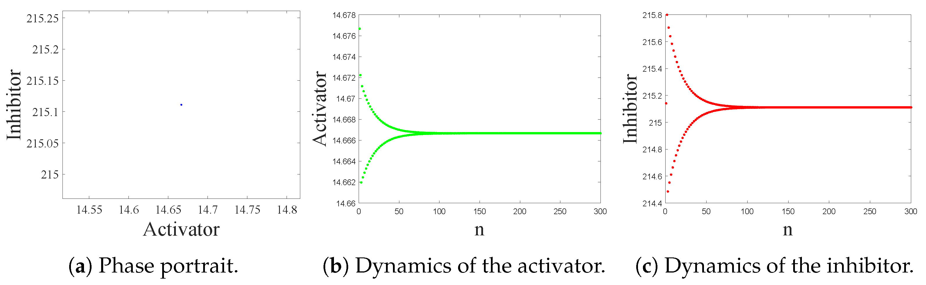
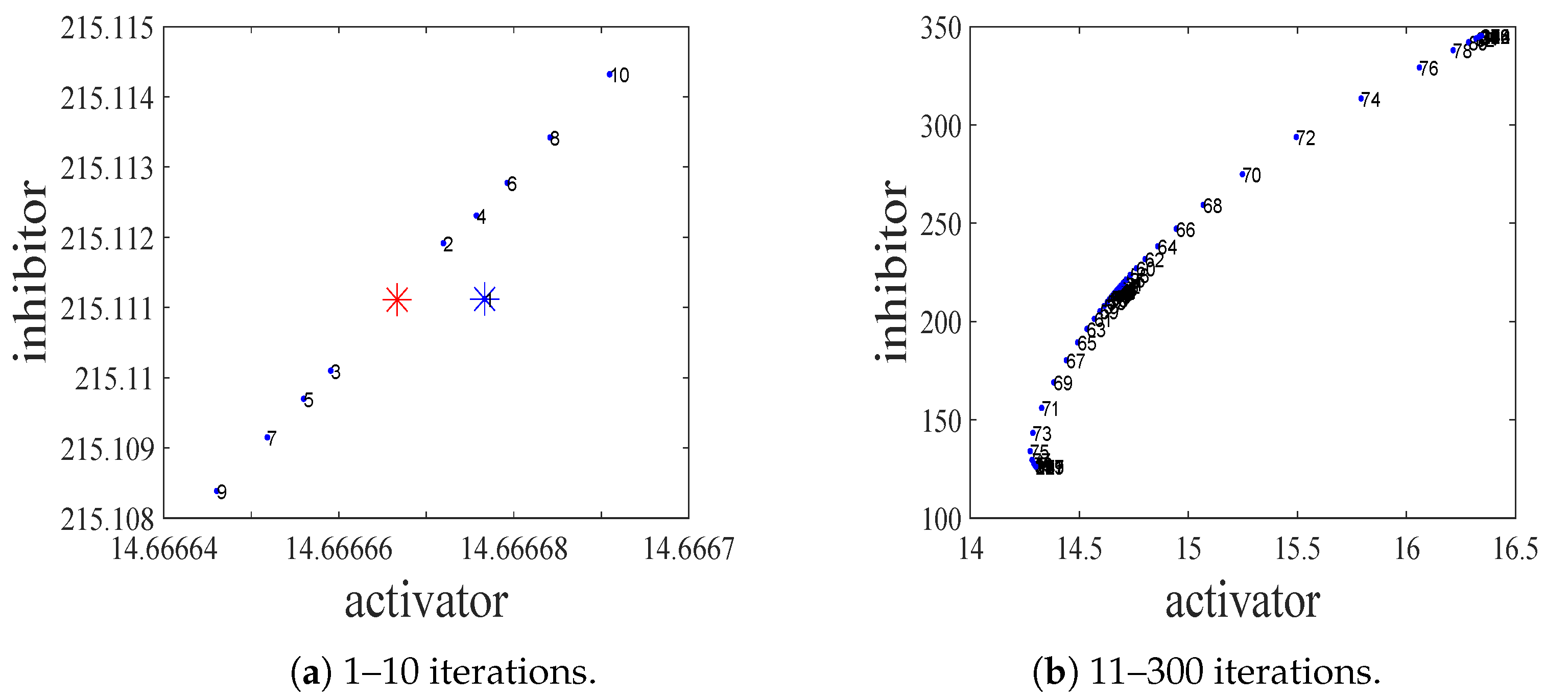
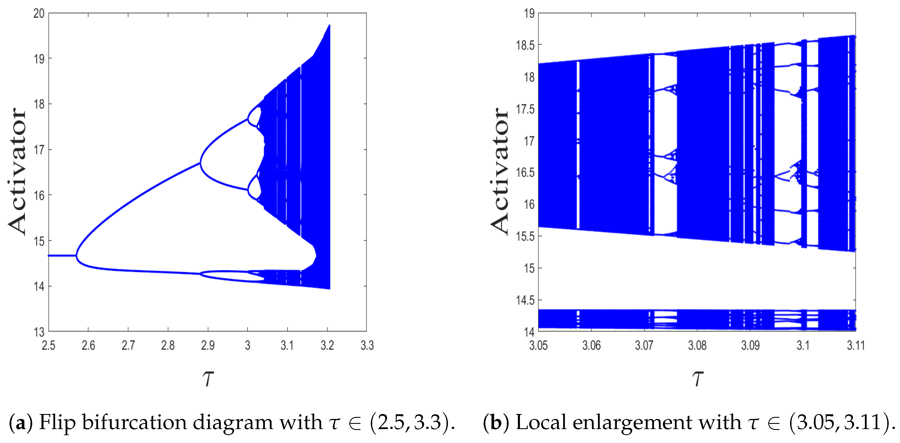
4.1. Kinetic Dynamics at Reaction Stage

At reaction stage, the kinetic behaviors of the CML model (4)–(7) can be described by the map (10), therefore, the simulations at this stage are about the map (10). We have obtained the theoretical results in Theorems 1 and 2; now, we give the related simulations.

Firstly, we give some illustrations about the Theorem 1. For the same type of fixed points, their dynamical behaviors are qualitatively consistent. Therefore, for the saddle, we only simulate the condition $\left(S{D}_2\right)$. For the stable node, we only simulate the condition $\left(S{N}_1\right)$. For the unstable node, we only simulate the condition $\left(U{N}_3\right)$. For the convenience of readers, the parameter values are listed in the following Table 1.

Table 1. The parameter values for illustrating the dynamics described by the Theorem 1.

Condition	$\mathit{\mu }$	${\mathit{c}}_0$	$\mathit{\tau }$	$({\mathit{a}}_{*},{\mathit{h}}_{*})$	${\mathit{\tau }}_1$	${\mathit{\tau }}_2$	${\mathit{c}}_1$	${\mathit{c}}_2$
$\left(S{N}_1\right)$	$0.3$	$3.4$	$2.5$	$(14.6667,215.1111)$	2.57048	5.1871	−0.7495	$1.9332$
$\left(S{D}_2\right)$	$0.3$	$3.4$	$2.7$	$(14.6667,215.1111)$	2.57048	5.1871	−0.7495	$1.9332$
$\left(U{N}_3\right)$	$0.3$	$3.4$	$5.2$	$(14.6667,215.1111)$	2.57048	5.1871	−0.7495	$1.9332$

When $\mu =0.3$, $c_0=3.4$, and $\tau =2.5$, the fixed point is $(a_{*},h_{*})=(14.6667,215.1111)$. Further calculations show that $c_2=1.9332$, ${\tau }_1=2.57048$. Obviously, the condition $\left(S{N}_1\right)$ holds. The eigenvalues of $J(a_{*},h_{*})$ are $-0.7895$ and $0.1132$. It indicates that the fixed point $(a_{*},h_{*})=(14.6667,215.1111)$ is a stable node, which supports the second conclusion in Theorem 1. In Figure 1a, we present the stable node $(a_{*},h_{*})$ in the phase space. As time changes, the orbit starting from $(16.6767,215.1411)$ is attracted to the fixed point $(a_{*},h_{*})=(14.6667,215.1111)$; please see Figure 1b,c.

Figure 1. The stable node of the map (10) with $\mu =0.3,c_0=3.4,\tau =2.5$.

When $\mu =0.3$, $c_0=3.4$, and $\tau =2.8$, condition $\left(S{D}_2\right)$ holds. The fixed point is $(a_{*},h_{*})=(14.6667,215.1111)$, and the eigenvalues of $J(a_{*},h_{*})$ are $-1.1786$ and $-0.0760$. Therefore, the fixed point $(a_{*},h_{*})$ is a saddle, which supports the first conclusion in Theorem 1. We choose an initial point $(a_{*}+0.0001,h_{*}+0.0001)$ in a small neighborhood of the fixed point $(a_{*},h_{*})$. The orbit starting from it goes far away from the fixed point $(a_{*},h_{*})$. This dynamical process is illustrated in Figure 2. The red asterisk in Figure 2a represents the saddle $(a_{*},h_{*})=(14.6667,215.1111)$, and the blue asterisk represents the initial point $(a_{*}+0.0001,h_{*}+0.0001)$. The blue dots represent the orbits in phase space, and the numbers next to the dots represent the number of iterations. From Figure 2b, we can see that the orbit will end up in two possible destinations. In fact, the two possible destinations are the period-2 points bifurcated from the fixed point via flip bifurcation.

Figure 2. The dynamical process of the saddle of the map (10) with $\mu =0.3,c_0=3.4,\tau =2.8$.

According to the Proposition 1 and the Theorem 2, the map (10) can undergo flip bifurcation when $\tau ={\tau }_1$. The flip bifurcation diagram is shown in Figure 3. When $\tau <{\tau }_1$, the fixed point is a stable node. When $\tau >{\tau }_1$, the stable node loses its stability, and firstly becomes a saddle if $\tau <{\tau }_2$. As $\tau$ increases and exceeds ${\tau }_2$, the fixed point becomes an unstable node.

Figure 3. Flip bifurcation diagram and its local enlargement of the activator for the map (10) with $\mu =0.3,c_0=3.4$.

In Figure 4, we present a graph of the evolution of the orbit over time from the vicinity of the saddle with $\tau =2.7$. The orbit starting from an initial point $(14.6767,215.1411)$ goes toward the period-2 points: $(14.34,142)$ and $(15.81,313.7)$. For the activator, please see Figure 4a, the orbit starting from $14.6767$ goes toward the points $14.34$ and $15.81$ and then jumps back and forth between them. For the inhibitor, please see Figure 4b, the orbit starting from $215.1411$ goes toward the points 142 and $313.7$ and then jumps back and forth between them.

Figure 4. The Kinetic dynamics of the period-2 orbit for activator and inhibitor of the map (10) with $\mu =0.3,c_0=3.4,\tau =2.7$. (a) Kinetic dynamics of the Period-2 orbit for activator. (b) Kinetic dynamics of the period-2 orbit for inhibitor.

When $\mu =0.3$, $c_0=3.4$, and $\tau =5.2$, we know that condition $U{N}_3$ holds. The eigenvalues of $J(a_{*},h_{*})$ are $-3.04593$ and $-1.00498$, therefore, the fixed point is an unstable node. In Figure 5, we illustrate the dynamical evolution of the orbit starting from the initial point $(a_{*}+0.00001,h_{*}+0.00001)$. The blue astersik represents the initial point (a_* + 0.00001, h_* + 0.00001). The blue dots represent the orbits in phase space and the numbers next to the dots represent the number of iterations. As the number of iterations increases, the orbit rapidly moves away from the fixed point and goes to infinity. From the simulation, we find that after only 16 iterations, the trajectory has already arrived at the level of the fourth power of 10.

Figure 5. The Kinetic dynamics of the unstable node of the map (10) with $\mu =0.3,c_0=3.4,\tau =5.2$.

Set $\mu =0.3,c_0=3.4$ and let $\tau$ vary from $2.5$ to $3.3$, then the map (10) experiences flip bifurcation. We draw the flip bifurcation diagram in Figure 3a and its local enlargement in Figure 3b, from which we can clearly observe the period doubling process and a series of periodic windows. When $\tau$ lies in the right neighborhood of ${\tau }_1=2.57048$, we can, for example, let $\tau =2.7$, $2.95$, $3.02$. We can see period-2, 4, 8 orbits. The corresponding phase portraits are shown in Figure 6.

Figure 6. The phase portraits of stable period-2, 4, 8 orbits of the map (10) with $\mu =0.3,c_0=3.4,$$\tau =2.7,2.95,3.02$ respectively.

As $\tau$ increases, more complex periodic orbits may appear, and the map (10) may even experience chaos. The maximum Lyapunov exponents are used to identify the chaotic behavior of the map (10). Corresponding to the flip bifurcation diagram (Figure 3a) and its local enlargement (Figure 3b), the maximum Lyapunov exponents and its local enlargement are plotted in Figure 7.

Figure 7. The maximum Lyapunov exponents corresponding to Figure 3 with $\mu =0.3,c_0=3.4$. (a) The maximum Lyapunov exponents with $\tau \in (2.5,3.3)$. (b) Local enlargement with $\tau \in (3.05,3.11)$.

Let $\tau =3.04$. We plot the phase portrait of the map (10) in Figure 8a, which demonstrates a complex period orbit. Let $\tau =3.065$ and $\tau =3.18$. According to Figure 7, we show two chaotic attractors in Figure 8b,d. Between chaotic behaviors, there exists a series of periodic windows. In each periodic window, there is a periodic orbit. Let $\tau =3.072$, we obtain the period-10 orbit in one of the periodic windows; please see Figure 8c.

Figure 8. The phase portraits about a complex periodic orbit and chaotic attractors of map (10) with $\mu =0.3,c_0=3.4$.

4.2. Turing Patterns of the CML Model

Since one of the conditions for the formation of Turing patterns is the existence of a stable homogeneous stationary state, we only focus on the stable conditions when we simulate the Turing patterns. According to the numerical simulations in Section 4.1, we know that the homogeneous stationary state can be a stable node or uniform periodic, quasi-periodic, and chaotic oscillatory states. Therefore, in this section, we mainly focus on the simulations of Turing patterns when different types of homogeneous stationary states lose their stability because of the diffusion terms. If the CML model undergoes only Turing bifurcation, then the induced Turing patterns are called pure Turing patterns. If the CML model undergoes both flip bifurcation and Turing bifurcation, then the induced Turing patterns are called flip-Turing patterns. In our CML model (4)–(7), there are both self-diffusion terms and cross-diffusion terms. The Turing instabilities are divided into self-diffusion-Turing instability and cross-diffusion-Turing instability. Therefore, we need to make clear whether the types of patterns induced by two types of diffusion-driven instabilities are different. We will explore this issue from a numerical perspective.

In order to demonstrate the Turing patterns of the CML model (4)–(7) induced by different mechanisms, we carry out the simulations under two different cases. In one case, the parameter values are $\mu =0.3$, $c_0=3.4$, $\delta =20$, $n=100$, $D_{a1}=0.1$, $D_{a2}=0$, $D_{h1}=0$, $D_{h2}=2$, which means that we only consider the effects of the self-diffusion terms. In another case, the parameter values are $\mu =0.3$, $c_0=3.4$, $\delta =20$, $n=100$, $D_{a1}=0$, $D_{a2}=0.001$, $D_{h1}=0.05$, $D_{h2}=0$, which means that we only consider the effects of the cross-diffusion terms.

Case I: $\mu =0.3$, $c_0=3.4$, $\delta =20$, $n=100$, $D_{a2}=0$, $D_{h1}=0$.

We first plot the $Z_m-\tau$ diagram in Figure 9a with $D_{a1}=0.1$ and $D_{h2}=2$. From Figure 9a, we find that the CML model undergoes Turing instability with ${\tau }^{\prime }=2.570585$. Furthermore, let $D_{a1}$ vary from 0 to 20 and $D_{h2}=2$, we plot the Turing instability regions in Figure 9b. Since the cross-diffusion terms are zero, namely, $D_{a2}=0$, $D_{h1}=0$, the pure Turing instability regions are formed only by self-diffusions. That is to say, the corresponding Turing patterns are induced by the pure-self-diffusion-Turing instability mechanism. Similarly, in the flip-Turing instability region, the corresponding Turing patterns are induced by the flip-self-diffusion-Turing instability mechanism.

Figure 9. The $Z_m-\tau$ diagram indicates the existence of Turing instability. The Turing instability regions indicate the different pattern formation mechanisms.

In the following, we will use numerical simulations to illustrate the Turing patterns induced by different mechanisms. All the simulations about the Turing patterns use the same initial conditions, which are given by random perturbations near the fixed point $(a_{*},h_{*})$. When $t=200,000$, the Turing patterns of the CML model exhibit stable static states. Since the patterns of the activators and inhibitors have similar morphologies, we only show the Turing patterns of the activators.

Let $D_{a1}=0.1$, $\tau =2.5$. According to Figure 9b, we know that the CML model will neither undergo a flip bifurcation nor a Turing bifurcation. It will stay in the stable homogeneous stationary state. At this moment, no Turing patterns can be produced, please see Figure 10a, the density of the activator in space is uniform. Now, we set $D_{a1}=10.2$ and still keep $\tau =2.5$. According to Figure 9b, we know that the CML model comes into the pure Turing instability region. It means that the CML model will only undergo a Turing bifurcation. The patterns are shown in Figure 10b. We can see a colorful, mottled grid pattern with winding and twisted bands. The patterns present natural curves in the bands and patchy distributions.

Figure 10. The stable homogeneous stationary state and the Turing patterns of the activators induced by the pure self-diffusion-Turing instability mechanism.

In the following, we let $\tau$ vary to make the homogeneous stationary state of the CML model stay at different stable states and illustrate the corresponding Turing patterns. Corresponding to the phase portraits in Figure 6 and Figure 8, we set $D_{a1}=0.1$, and let $\tau =2.7$, $\tau =2.95$, $\tau =3.02$, $\tau =3.04$, $\tau =3.72$ and $\tau =3.18$ respectively. Therefore, in Figure 11 we show the transformations in activator patterns that occur with the period-doubling process.

Figure 11. The Turing patterns of the activators induced by the flip-self-diffusion-Turing instability mechanism.

According to Figure 9b, for $\tau =2.7>{\tau }_1\approx {\tau }^{\prime }\approx 2.57$, the homogenous steady state is no longer a stable node; it is a stable period-2 orbit. In this situation, the CML model undergoes both flip bifurcation and Turing bifurcation simultaneously. The corresponding Turing patterns are shown in Figure 11a, from which we can observe a Turing pattern consisting of two alternating colors of patches. In fact, the two colors of patches are the period-2 points: $14.34$ and $15.81$. Similarly, when $\tau =2.95$, the CML model also undergoes flip-Turing instability. The corresponding Turing patterns are shown in Figure 11b, from which we can observe a Turing pattern consisting of four colors of patches. The four colors of patches are the period-4 points. These repeatedly alternating states of the activators intertwined with each other. When $\tau =3.02$, we can see a Turing pattern consisting of eight alternating colors of patches; please see Figure 11c. For some $\tau$ values, we can observe patterns intertwined with patches of 16 colors, as well as patterns intertwined with patches of 32 colors. Here, we will not present them further. As $\tau$ increases, the number of colors in the pattern will continue to double. The fragmentation of the pattern will also gradually increase. For example, let $\tau =3.04$ and $\tau =3.072$, we can see more complex Turing patterns with multiple states interwoven, please see Figure 11d,e. For $\tau =3.18$, the Turing patterns enter into spatiotemporal chaos—please see Figure 11f—from which we can see that the patterns are fragmented to a greater extent. From Figure 11, we can see that as $\tau$ increases, the Turing patterns gradually change from ordered to disordered, and the degree of disorder becomes higher and higher. These pattern mechanisms are called flip-self-diffusion-Turing instability mechanism.

It is worth noting that all the above Turing patterns are formed under the effects of self-diffusions. We know that when $D_{a1}=0.1$ and $\tau =2.5$, according to the Figure 9b and Figure 11a, the CML model has a uniform distribution in space. Now, we let the cross-diffusion coefficients be positive. For example, when $D_{a2}=0.1$, $D_{h1}=0.2$, we find that the CMLs model can undergo Turing instability, and the Turing patterns are exhibited in Figure 12. The patterns are induced by the pure-cross-diffussion-Turing instability. The corresponding mechanism is called the pure-cross-diffusion-Turing instability mechanism. From Figure 12, we can see dense patches and twisted bands nested together. Compared to the patterns induced by the pure-self-diffusion-Turing instability mechanism, the patterns induced by the pure-cross-diffusion-Turing instability mechanism exhibit a more complex structure. To some extent, this pattern resembles the markings on the skin of certain animals.

Figure 12. The Turing patterns of the activator induced by pure-cross-diffusion-Turing instability mechanism with $D_{a1}=0.1$, $\tau =2.5$, $D_{a2}=0.1$, $D_{h1}=0.2$.

Case II: $\mu =0.3$, $c_0=3.4$, $\delta =20$, $n=100$, $D_{a1}=0$, $D_{h2}=0$.

We first plot the $Z_m-\tau$ diagram in Figure 13a with $D_{a2}=0.001$ and $D_{h1}=0.05$. We find that the CML model undergoes Turing instability with ${\tau }^{\prime }=2.570483$. Furthermore, let $D_{a2}$ vary from 0 to 1, we plot the Turing instability regions in Figure 13b.

Figure 13. The $Z_m-\tau$ diagram indicates the existence of Turing instability. The Turing instability regions indicate the different pattern formation mechanisms.

In the following, we will use numerical simulations to illustrate the Turing patterns induced by different mechanisms. All the simulations about the Turing patterns use the same initial conditions, which are given by random perturbations near the fixed point $(a_{*}=14.6667,h_{*}=215.1411)$. When $t=200,000$, the Turing patterns of the CML model exhibit stable static states. Since the patterns of the activators and inhibitors have similar morphologies, we only show the Turing patterns of the activators.

Let $D_{a2}=0.001$, $D_{h1}=0.05$, and $\tau =2.5$. According to Figure 13b, we know that the CML model will neither undergo a flip bifurcation nor a Turing bifurcation. It will stay in the homogeneous stationary state, namely, the stable node. At this moment, no Turing patterns can be induced; please see Figure 14a, the density of the activator in space is uniform. Let other parameters be fixed, and change the value of $\tau$, then we illustrate the Turing patterns induced by the couple of flip bifurcation and Turing bifurcation.

Figure 14. The Turing patterns of the activator induced by the flip-corss-diffusion Turing instability mechanism.

Let $\tau =2.7$. Then, $\tau >{\tau }_1$ and $\tau >{\tau }^{\prime }$; it means that the CML model can experience both flip bifurcation and Turing bifurcation. The corresponding Turing patterns are shown in Figure 14b. Similarly, the patterns consist of two alternative states, namely, the period-2 orbit bifurcated from the fixed point via flip bifurcation. Furthermore, let $\tau =2.95$ and $\tau =3.02$, we can see that the colors consisting of the patterns are doubling. Please see Figure 14c,d. When $\tau =3.04$, the homogeneous stationary state is a complex period orbit, the corresponding patterns are more fragmented than the others, please see Figure 14e. When $\tau =3.072$, the homogeneous stationary state is a period-10 orbit lying in a periodic window; the corresponding patterns are shown in Figure 14f. All these Turing patterns shown in Figure 14 are induced by the flip-cross-diffusion-Turing instability mechanism.

Next, we will illustrate the Turing patterns induced by the pure-cross-diffusion-Turing instability mechanism. Let $D_{a2}=0.03$, $D_{h1}=0.05$, and $\tau =2.5$; according to Figure 13b, we know that the CML model will only undergo a Turing bifurcation. The patterns are shown in Figure 15, and the corresponding mechanism is called the pure-cross-diffusion Turing instability mechanism. From Figure 15, we can also see a colorful mottled grid pattern with winding and twisted bands.

Figure 15. The Turing patterns of the activator induced by the pure-cross-diffusion-Turing instability mechanism with $D_{a2}=0.03$, $D_{h1}=0.05$, $\tau =2.5$.

Finally, we will illustrate the Turing patterns induced by the pure-self-diffusion-Turing instability mechanism. We assume that cross-diffusion acts first in the system. But cross-diffusion does not cause Turing instability. The values of the parameters are the same as in the simulations depicted in Figure 14a. Then self-diffusion terms are added to the system, namely, $D_{a1}=10.2$ and $D_{h2}=2$, but at that point, the CML model undergoes Turing instability and Turing patterns are formed. Please see Figure 16.

Figure 16. The Turing patterns of the activator induced by the pure-self-diffusion-Turing instability mechanism with $D_{a1}=10.2$, $D_{a2}=0.001$, $D_{h1}=0.05$, $D_{h2}=2$ and $\tau =2.5$.

5. Discussion and Conclusions

This paper employs the coupled map lattices method to establish a spatiotemporally discrete activator–inhibitor model with self- and cross-diffusions. We apply the classical theory of bifurcations and standard bifurcation analysis methods to investigate the bifurcations, chaos, and pattern formations of the CML model (4)–(7). In addition to the standard bifurcation analysis, we specifically studied the numerical effects of cross-diffusion on pattern formation. Previously, many research works on pattern formation of activator–inhibitor models have been undertaken, including the works in [32,33,35,40,44,45,46] and the references therein. From the theoretical analysis and numerical simulations, and by comparing with the existing approaches, we find that the CML model can exhibit complex nonlinear behaviors and new spatiotemporal dynamical phenomena. Based on the comparison with former studies, the following aspects are disscussed and emphasized for the improvement of the present paper.

•

It is worth noting that, compared to the paper [46], our model in this paper includes an additional cross-diffusion term. In terms of spatially homogeneous dynamic behavior, the authors in [46] have already proven the existence and stability of a positive fixed point and have conducted an analysis of flip bifurcation and Neimark–Sacker bifurcation. Our work is similar to the spatially homogeneous dynamic behavior discussed in [46], while we have further discussed the types of the fixed point and determined the precise parameter conditions for the fixed point to be a saddle, a stable node, and an unstable node. For spatially heterogeneous dynamic behavior, the authors in [46] only explored the instability phenomena caused by self-diffusion, whereas our research not only analyzed the instability caused by self-diffusion but also considered the instability induced by cross-diffusion. Therefore, the mechanisms of pattern formation we have revealed are more comprehensive, and the types of patterns observed are also more abundant. For example, in our paper, the pure-self-Turing instability mechanism leads to a colorful mottled grid pattern with winding and twisted bands. The pure-cross-Turing instability mechanism leads to dense patches and twisted bands nested together. These patterns cannot be generated by the model in [46]. Furthermore, our system can also undergo a Neimarck–Sacker bifurcation. We have conducted related research on this and discovered some very interesting phenomena such as a plum blossom-shaped chaotic attractor. Moving forward, we will continue to delve deeper into this field. Compared to the continuous Gierer–Meinhardt model, our CML-based Gierer–Meinhardt model exhibits a richer dynamic behavior. Our model undergoes a flip bifurcation, which is not observed in the corresponding continuous model. The mechanisms of pattern formation in our model are more diverse than those in the corresponding continuous models [32,33,44,45]. Additionally, the types of patterns we observe are also more abundant.

•

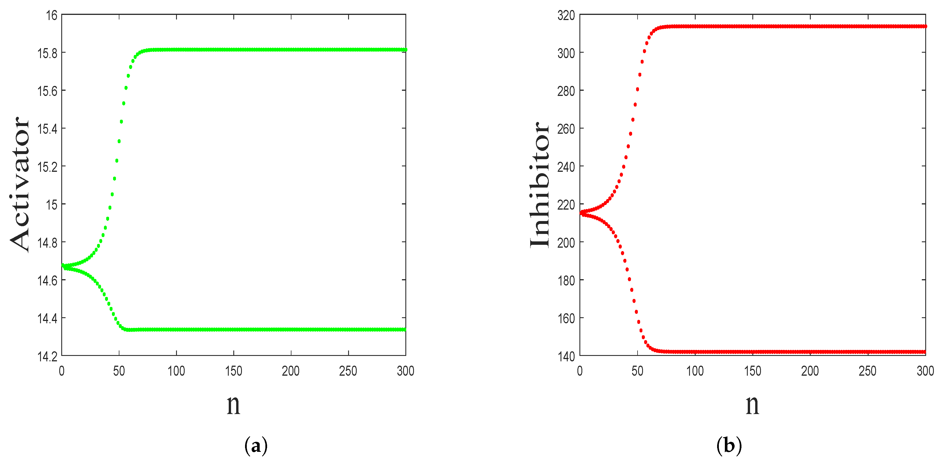
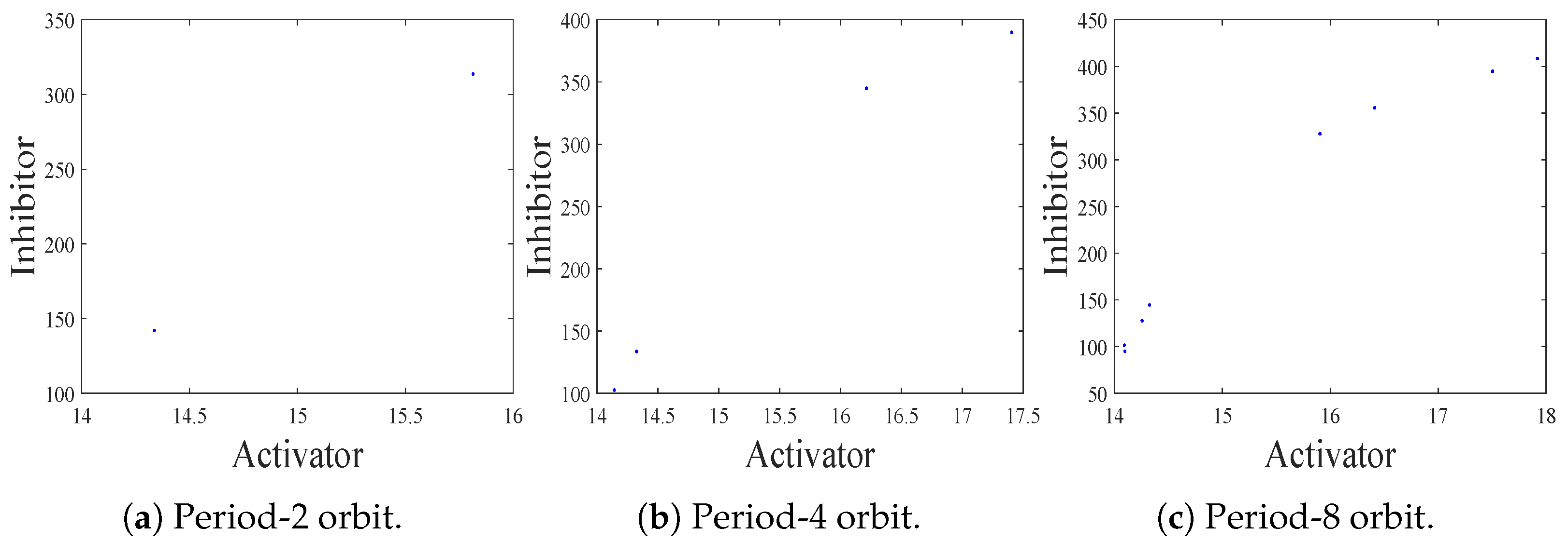
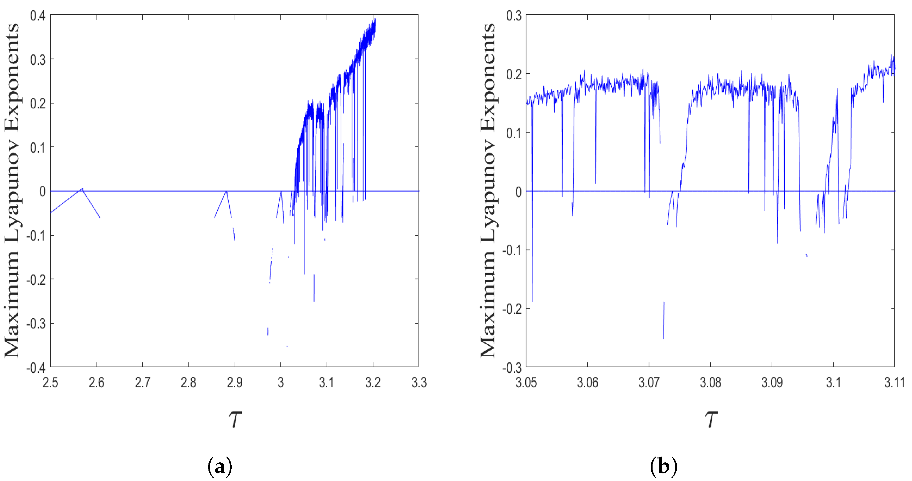
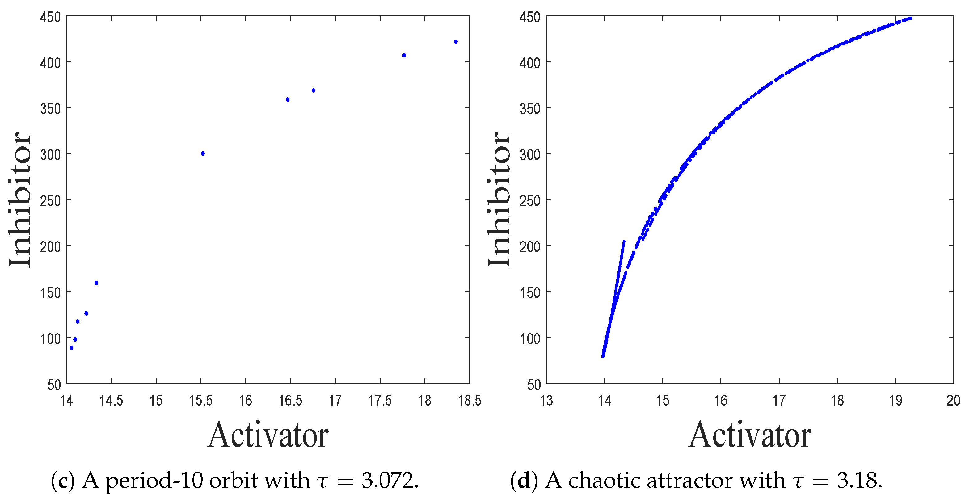
The spatiotemporal dynamics of the CML model (4)–(7) consists of two parts: spatially homogeneous and spatially heterogeneous dynamics. The spatially homogeneous dynamics includes a stable homogeneous stationary state (stable node) as well as homogeneous oscillatory states generated by flip bifurcation. The spatially heterogeneous dynamics include the patterns induced by Turing instability. In this paper, we give the precise parameter conditions for the system to experience flip bifurcation, which induces a continuous period-doubling oscillatory process and introduces a path to chaos, allowing the system to enter a chaotic oscillatory state eventually. The maximum Lyapunov exponents can help us to distinguish the regular and irregular behaviors. On the road to chaos, we can see many periodic windows. In each window, there exists a periodic orbit.

•

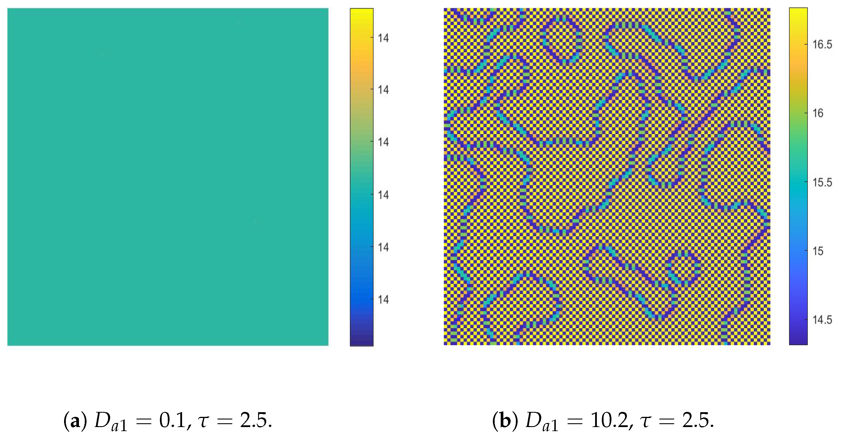
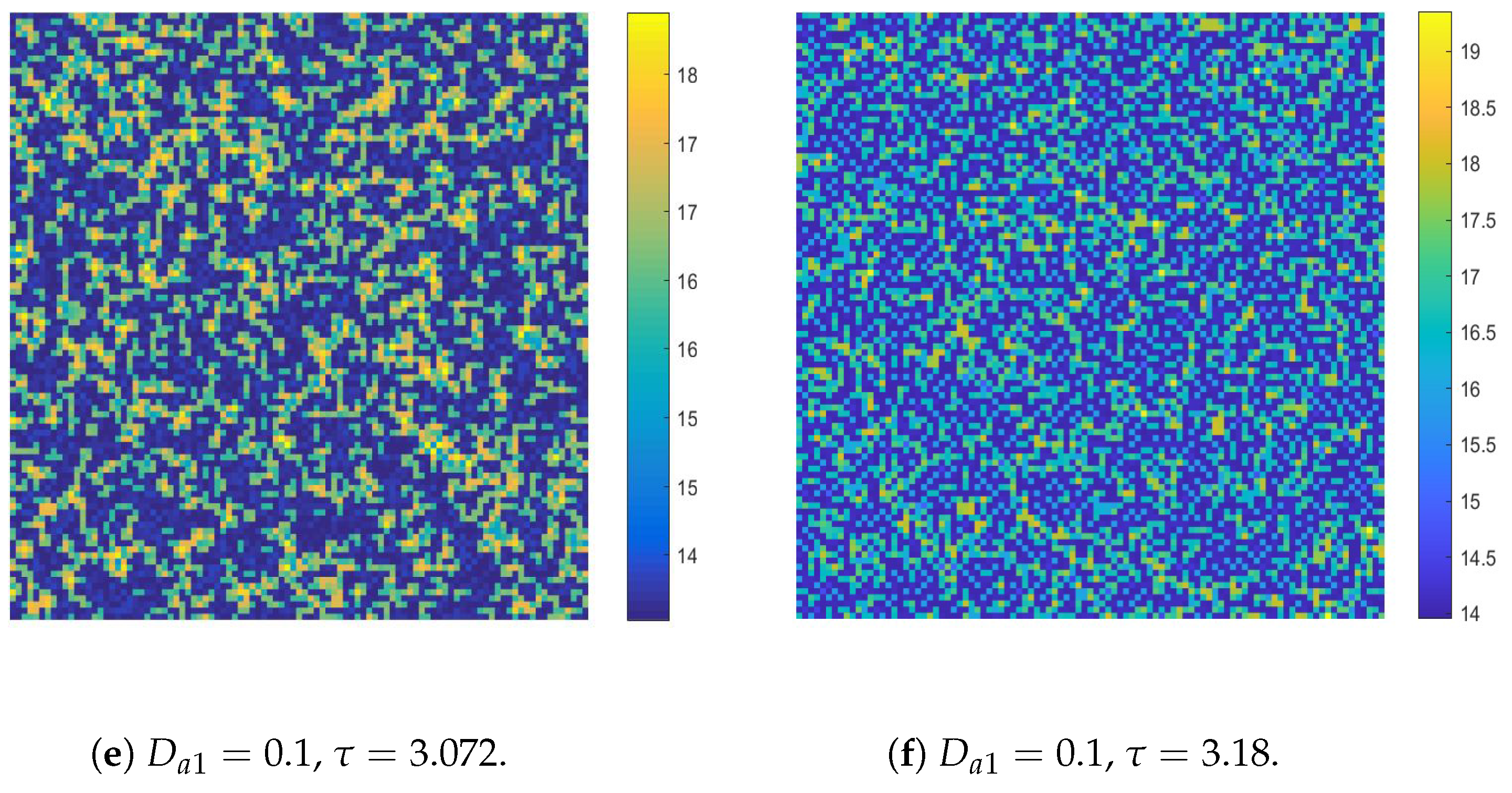
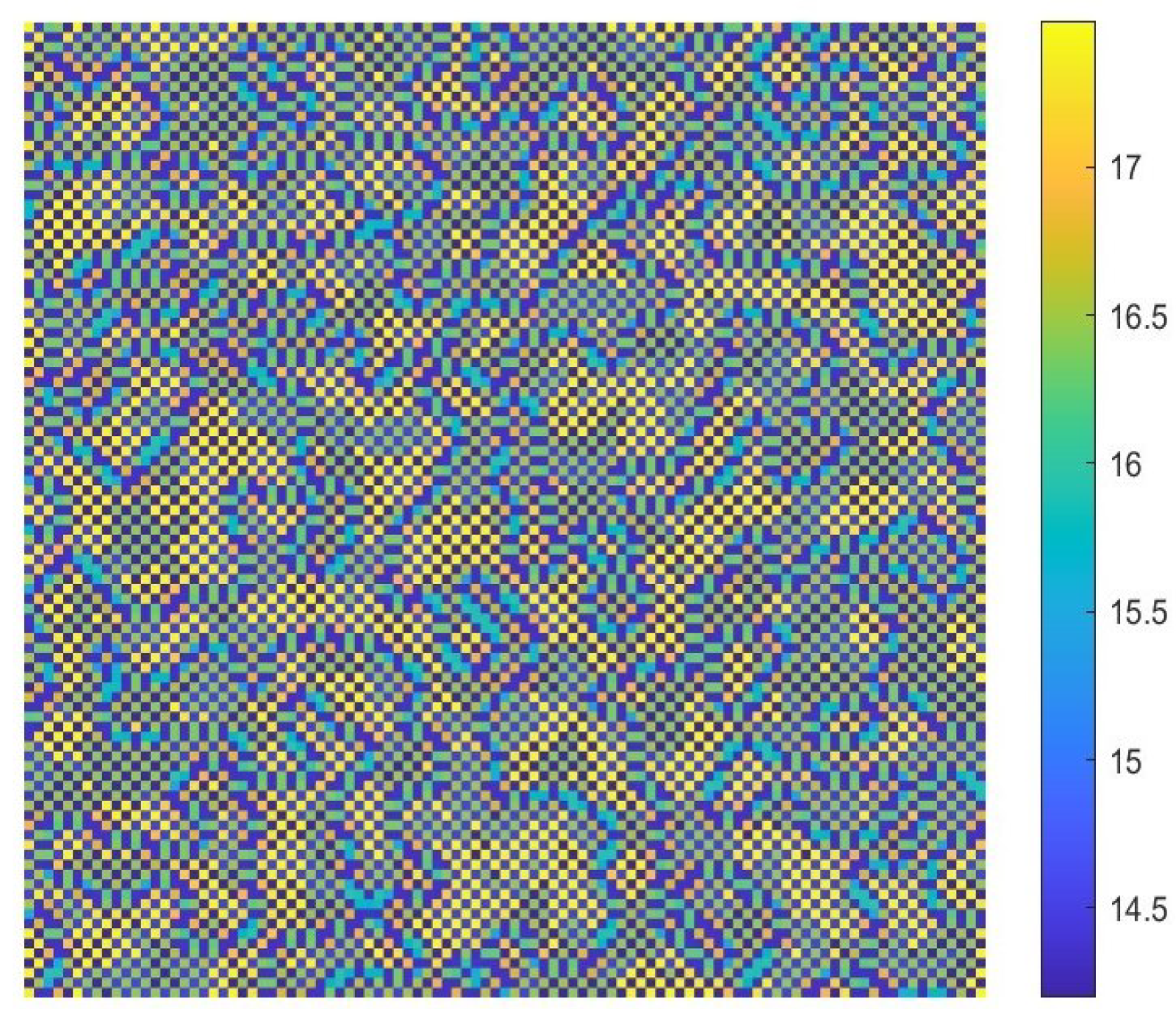
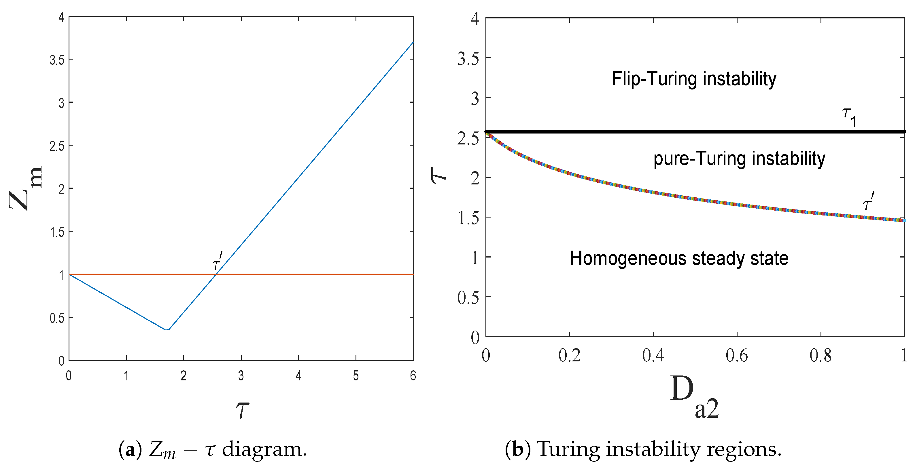
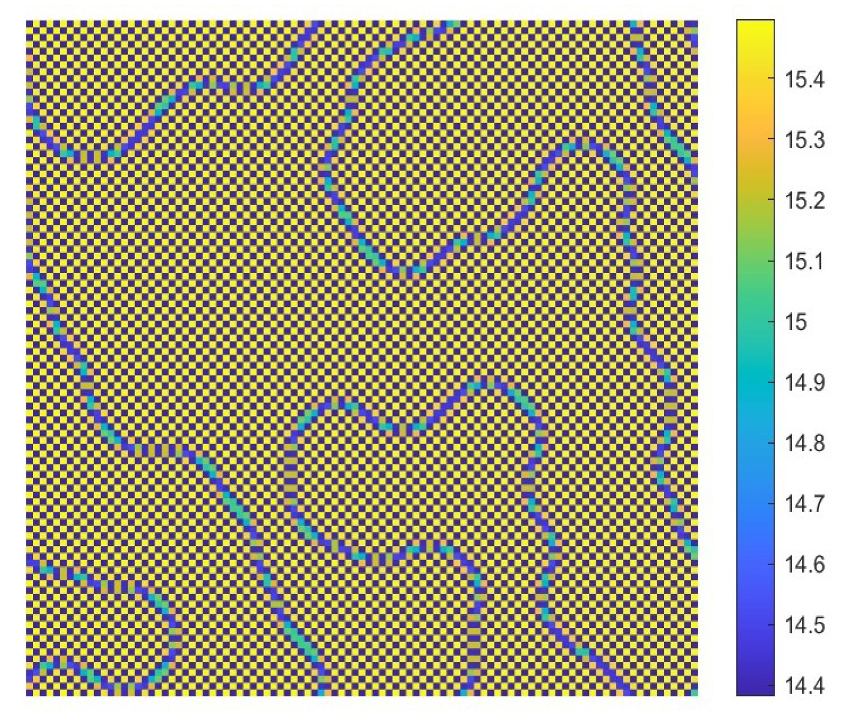
The diffusion effects offer the possibility for the emergence of Turing bifurcation, while the homogeneous state of kinetic dynamical behavior offers the options for the CML model. During the numerical simulations, we find that the size of the Turing region is related to the spatial step $\delta$. The mechanisms for the pattern formation of the CML model are divided into two broad categories: pure Turing instability mechanism and flip-Turing instability mechanism. The pure Turing instability mechanism can be further categorized into pure-self-diffusion-Turing instability mechanism and pure-cross-diffusion-Turing instability mechanism. The flip-Turing instability mechanism can be further categorized into the flip-self-diffusion-Turing instability mechanism and flip-cross-diffusion-Turing instability mechanism. The pure-self-Turing instability mechanism leads to a colorful, mottled grid pattern with winding and twisted bands. The pure-cross-Turing instability mechanism leads to dense patches and twisted bands nested together. The flip-Turing instability mechanism leads to multi-state intertwined patterns. The chaos-self-diffusion-Turing instability mechanism leads to labyrinthine and mosaic patterns. The flip-Turing instability mechanism on chaotic paths induces a spatial multiply periodization process. It leads to a pattern transition of the CML model from spatiotemporally ordered patterns to spatiotemporally disordered patterns.

•

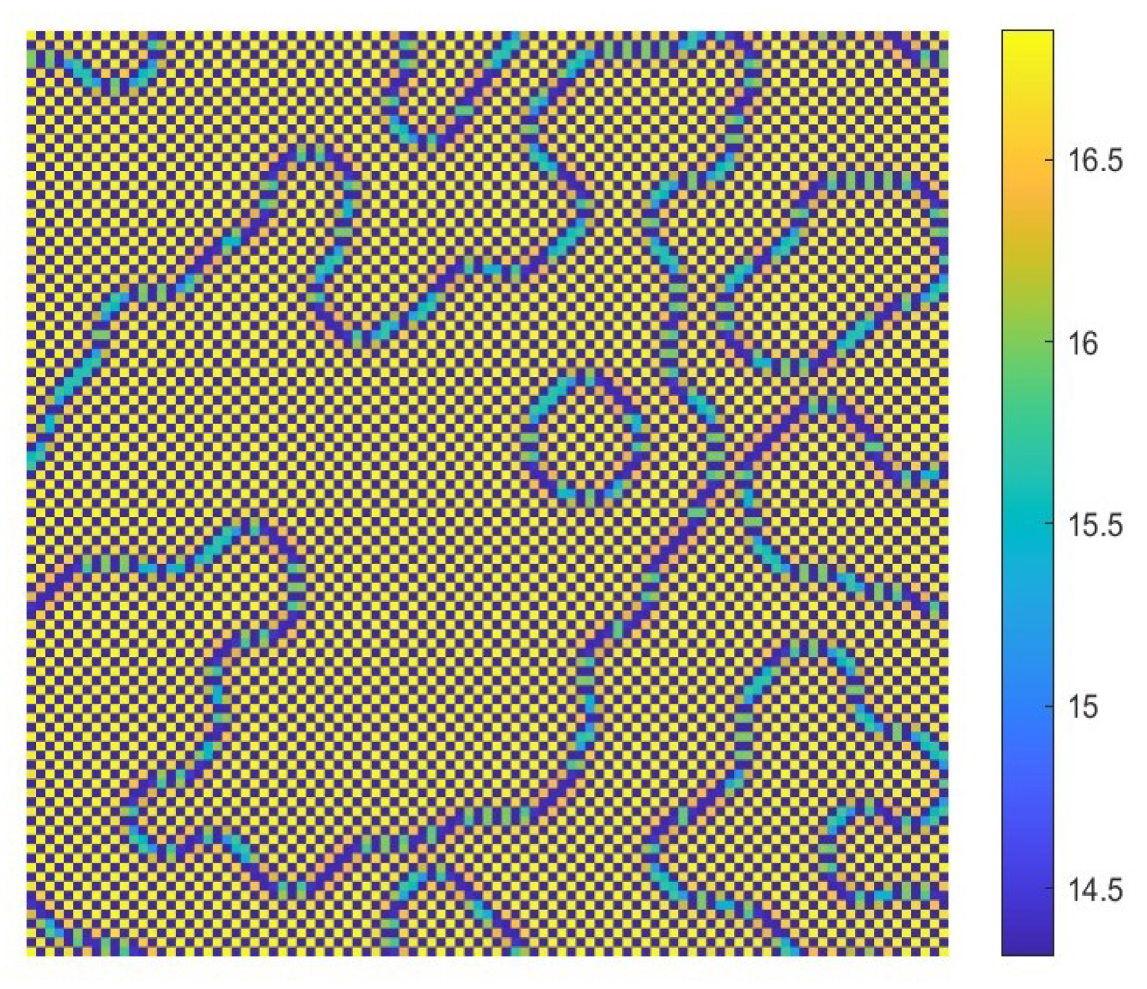
Self-diffusion and cross-diffusion can both lead to Turing instability, thereby forming Turing patterns. When the system only has self-diffusion or only cross-diffusion, the resulting spatial patterns are shown in Figure 10b and Figure 15. They are all mottled grid patterns with winding and twisted bands. The patterns present natural curves in the bands and patchy distributions. However, when the system has both self-diffusion and cross-diffusion if the instability phenomenon and the formation of the patterns are primarily caused by cross-diffusion, as shown in Figure 12, the resulting spatial patterns are dense patches and twisted bands nested together. If the instability phenomenon and the formation of the patterns are primarily caused by self-diffusion, as shown in Figure 16, the resulting spatial patterns are also mottled grid patterns with winding and twisted bands. The complexity of the pattern structure in Figure 12 is higher than that in Figure 16.

•

The Turing patterns formed each time under random perturbations are qualitatively consistent but not identical in shape. From the simulations, we find that the patterns induced by pure-cross-diffusion-Turing instability mechanism are more coplexed than the patterns induced by pure-self-diffusion-Turing instability mechanism. It is important to note in particular that when $\tau =3.18$ in the second case. For the map (10), there exists a chaotic attractor, as shown in Figure 8d. But when we consider the effects of the pure cross-diffusion effects, though the CML model (4)–(7) experiences Turing instability, while we can not find the corresponding mosaic patterns similar to the patterns shown in Figure 11 which are induced by the pure-self-diffusion effects.

Although the coupled map lattice (CML) method has been widely applied in the study of dynamic systems, we believe that research introducing cross-diffusion terms into reaction–diffusion systems is still relatively rare. The CML method demonstrates its unique advantages in this study, particularly in accurately simulating reaction–diffusion systems with cross-diffusion on a discretized grid, and effectively capturing the complex dynamics of pattern formation. This approach provides a new perspective for studying how cross-diffusion induces irregular patterns.

Our study provides a perspective on the relationship between bifurcation, chaos, and pattern formation and reveals the common laws of pattern formation and transformation in activator–inhibitor systems with self- and cross-diffusion systems based on CML models. These laws provide a theoretical basis for further exploration of spatiotemporal complexity in spatiotemporally discrete embryonic developmental systems. Due to their relevance to similar research issues, the theoretical framework and analytical techniques elaborated within this research could potentially be applied to a wider range of fields. This includes, but is not limited to, ecological dynamics in complex ecosystems, pattern formation and self-organization in physical and biological systems, the spatial distribution of vegetation, and the statistical mechanics of evolutionary and coevolutionary game theory.

References

- Murray, J.D. Mathematical Biology I: An Introduction, 3rd ed.; Springer: New York, NY, USA, 2002. [Google Scholar]
- Turing, A.M. The chemical basis of morphogenesis. Philpos. Trans. R. Soc. Lond. Ser. B 1952, 237, 37–72. [Google Scholar]
- Gierer, A.; Meinhardt, H. A theory of biological pattern formation. Kybernetik 1972, 12, 30–39. [Google Scholar] [CrossRef]
- Gao, S.P.; Chang, L.L.; Perc, M.; Wang, Z. Turing patterns in simplicial complexes. Phys. Rev. E 2023, 107, 014216. [Google Scholar] [CrossRef]
- Vanag, V.K.; Epstein, I.R. Pattern formation in a tunable medium: The Belousov-Zhabotinsky reaction in an aerosol OT microemulsion. Phys. Rev. Lett. 2001, 87, 169–177. [Google Scholar] [CrossRef]
- Tan, Z.; Chen, S.; Peng, X.; Zhang, L.; Gao, C. Polyamide membranes with nanoscale Turing structures for water purification. Science 2018, 360, 518–521. [Google Scholar] [CrossRef]
- Karig, D.; Martini, K.M.; Lu, T.; Delateur, N.A.; Goldenfeld, N.; Weiss, R. Stochastic Turing patterns in a synthetic bacterial population. Proc. Natl. Acad. Sci. USA 2018, 115, 6572–6577. [Google Scholar] [CrossRef]
- Wakano, J.Y.; Nowak, M.A.; Hauert, C. Spatial dynamics of ecological public goods. Proc. Natl. Acad. Sci. USA 2009, 106, 7910–7914. [Google Scholar] [CrossRef]
- Short, M.B.; Bertozzi, A.L.; Brantingham, P.J. Nonlinear patterns in urban crime: Hotspots, bifurcations, and suppression. SIAM J. Appl. Dyn. Syst. 2010, 9, 462–483. [Google Scholar] [CrossRef]
- Fuseya, Y.; Katsuno, H.; Behnia, K.; Kapitulnik, A. Nanoscale Turing patterns in a bismuth monolayer. Nat. Phys. 2021, 17, 1031–1036. [Google Scholar] [CrossRef]
- Taylor, N.P.; Kim, H.; Krause, A.L.; Van Gorder, R.A. A non-local cross-diffusion model of population dynamics I: Emergent spatial and spatiotemporal patterns. Bull. Math. Biol. 2020, 82, 112. [Google Scholar] [CrossRef]
- Hata, S.; Nakao, H.; Mikhailov, A.S. Dispersal-induced destabilization of metapopulations and oscillatory Turing patterns in ecological networks. Sci. Rep. 2014, 4, 3585. [Google Scholar] [CrossRef]
- Kondo, S.; Miura, T. Reaction-diffusion model as a framework for understanding biological pattern formation. Science 2010, 329, 1616–1620. [Google Scholar] [CrossRef]
- Nakamasu, A.; Takahashi, G.; Kanbe, A.; Kondo, S. Interactions between zebrafish pigment cells responsible for the generation of Turing patterns. Proc. Natl. Acad. Sci. USA 2009, 106, 8429–8434. [Google Scholar] [CrossRef]
- Alessio, B.M.; Gupta, A. Diffusiophoresis-enhanced Turing patterns. Sci. Adv. 2023, 9, eadj2457. [Google Scholar] [CrossRef]
- Rui, X.; Gao, Q.Y.; Azaele, S.; Sun, Y.Z. Effects of noise on the critical points of Turing instability in complex ecosystems. Phys. Rev. E 2023, 108, 014407. [Google Scholar]
- Huang, T.S.; Zhang, H.Y. Bifurcation, chaos and pattern formation in a space- and time-discrete predator-prey system. Chaos Solitons Fractals 2016, 91, 92–107. [Google Scholar] [CrossRef]
- Li, Y.; Cao, J.J.; Sun, Y.; Song, D.; Wu, X.Y. Spatiotemporal patterns induced by four mechanisms in a tussock sedge model with discrete time and space variables. Adv. Differ. Equ. 2021, 399, 92–107. [Google Scholar] [CrossRef]
- Nakao, H.; Mikhailov, A.S. Turing patterns in network organized activator inhibitor systems. Nat. Phys. 2010, 6, 544–550. [Google Scholar] [CrossRef]
- Horsthemke, W.; Lam, K.; Moore, P.K. Network topology and Turing instabilities in small arrays of diffusively coupled reactors. Phys. Lett. A 2004, 328, 444–451. [Google Scholar] [CrossRef]
- Zheng, Q.Q.; Shen, J.W.; Horsthemke, Y.W.; Lam, K.; Moore, P.K. Turing instability in the reaction-diffusion network. Phys. Rev. E 2020, 102, 1–9. [Google Scholar] [CrossRef]
- Li, Z.J.; Fang, S.Y.; Ma, M.L.; Wang, M.J. Bursting Oscillations and Experimental Verification of a Rucklidge System. Int. J. Bifurcat. Chaos 2021, 31, 1–13. [Google Scholar] [CrossRef]
- Mistro, D.C.; Rodrigues, L.A.D.; Petrovskii, S. Spatiotempral complexity of biological invasion in a space and time discrete predator-prey system with strong Allee effect. Ecol. Complex 2012, 9, 16–32. [Google Scholar] [CrossRef]
- Rodrigues, L.A.D.; Mistro, D.C.; Petrovskii, S. Pattern formation in a space- and time-discrete predator-prey system with strong Allee effect. Theor. Ecol. 2012, 12, 43–57. [Google Scholar] [CrossRef]
- Kaneko, K. Pattern dynamics in spatiotemporal chaos: Pattern secletion, diffusion of defect and pattern competition intermettency. Physica D 1989, 34, 1–41. [Google Scholar] [CrossRef]
- Kaneko, K. Spatiotemporal chaos in one and two dimensional coupled map lattices. Physica D 1989, 37, 60–82. [Google Scholar] [CrossRef]
- Han, Y.T.; Han, B.; Zhang, L.; Xu, L.; Li, M.F.; Zhang, G. Turing instability and wave patterns for a symmetric discrete competitive Lotka-Volteera system. WSEAS Trans. Math. 2011, 10, 181–189. [Google Scholar]
- May, R.M. Simple mathematical models with very complicated dynamics. Nature 1976, 261, 459–467. [Google Scholar] [CrossRef]
- Liu, X.; Xiao, D. Complex dynamic behaviors of a discrete-time predator prey system. Chaos Solition Fractals 2007, 32, 80–94. [Google Scholar] [CrossRef]
- Woodward, D.E.; Tyson, R.; Myerscough, M.R.; Murray, J.D.; Budrene, E.O.; Berg, H.C. Spatio-Temporal Patterns Generated by Salmonella typhimurium. Biophys. J. 1995, 68, 2181–2189. [Google Scholar] [CrossRef]
- Brenner, M.P.; Levitov, L.S.; Budrene, E.O. Physical Mechanisms for Chemotactic Pattern Formation by Bacteria. Biophys. J. 1998, 74, 1677–1693. [Google Scholar] [CrossRef]
- Li, Y.; Wang, J.L.; Hou, X.J. Stripe and spot patterns for general Gierer-Meinhardt model with common sources. Int. J. Bifurcat. Chaos 2017, 27, 1750018. [Google Scholar] [CrossRef]
- Li, Y.; Wang, J.L.; Hou, X.J. Stripe and spot patterns for Gierer-Meinhardt model with saturated activator production. J. Math. Anal. Appl. 2017, 449, 1863–1879. [Google Scholar] [CrossRef]
- Liu, J.; Yi, F.; Wei, J. Multiple bifurcation analysis and spatiotemporal patterns in a 1-d geierer meinhardt model of morphogenesis. Int. J. Bifurcat. Chaos 2010, 20, 1007–1025. [Google Scholar] [CrossRef]
- Wu, R.; Zhou, Y.; Shao, Y.; Chen, L. Bifurcation and turing patterns of reaction-diffusion activator-inhibitor model. Physica A 2017, 482, 597–610. [Google Scholar] [CrossRef]
- Zhong, S.; Wang, J.L.; Xia, J.D.; Li, Y. Spatiotemporal dynamics and pattern formations of an activator-substrate model with double saturation terms. Int. J. Bifurc. Chaos 2021, 31, 2150129. [Google Scholar] [CrossRef]
- Yang, R.; Yu, X. Turing-Hopf bifurcation in diffusive Gierer-Meinhardt model. Int. J. Bifurc. Chaos 2022, 32, 2250046. [Google Scholar] [CrossRef]
- Ma, X.Y.; Wang, J.L.; Zhu, Y.H.; Wang, Z.W.; Sun, Y. Turing-Hopf Bifurcation Coinduced by Diffusion and Delay in Gierer-Meinhardt Systems. Int. J. Bifurc. Chaos 2024, 34, 2450162. [Google Scholar] [CrossRef]
- Zhao, S.; Wang, H.; Jiang, W. Turing-Hopf bifurcation and spatiotemporal patterns in a Gierer-Meinhardt system with gene expression delay. Nonlinear Anal. Model. Control 2021, 26, 461–481. [Google Scholar] [CrossRef]
- Zhao, S.; Wang, H. Turing–Turing bifurcation and multi-stable patterns in a Gierer–Meinhardt system. Appl. Math. Model 2022, 112, 632–648. [Google Scholar] [CrossRef]
- Wu, R.C.; Yang, L.L. Bogdanov-Takens Bifurcation of Codimension 3 in the Gierer-Meinhardt Model. Int. J. Bifurc. Chaos 2023, 33, 2350163. [Google Scholar] [CrossRef]
- Lv, J.P.; Jing, H.F. Analyzing the dynamic behavior of the Gierer-Meinhardt model using finite difference method. AIP Adv. 2024, 14, 085215. [Google Scholar] [CrossRef]
- Mai, F.X.; Qin, L.J.; Zhang, G. Turing instability for a semi-discrete Gierer Meinhardt system. Physica A 2012, 391, 2014–2022. [Google Scholar] [CrossRef]
- Wang, J.L.; Li, Y.; Zhong, S.H.; Hou, X.J. Analysis of bifurcation, chaos and pattern formation in a discrete time and space Gierer Meinhardt system. Chaos Solitons Fractals 2019, 118, 1–17. [Google Scholar] [CrossRef]
- Zhu, Y.H.; Li, Y.; Ma, X.Y.; Sun, Y.; Wang, Z.W.; Wang, J.L. Bifurcation and Turing Pattern Analysis for a Spatiotemporal Discrete Depletion Type Gierer-Meinhardt Model with Self-Diffusion and Cross-Diffusion. J. Appl. Anal. Comput. 2025, 15, 705–733. [Google Scholar]
- Liu, B.; Wu, R.C. Bifurcation and Patterns Analysis for a Spatiotemporal Discrete Gierer-Meinhardt System. Mathematics 2022, 10, 243. [Google Scholar] [CrossRef]
- Nakata, K.; Sokabe, M.; Suzuki, R. The application of the Gierer Meinhardt equations to the development of the retinotectal projection. Biol. Cybern 1979, 35, 235–241. [Google Scholar] [CrossRef]
- Meinhardt, H. Models of Biological Pattern Formation; Academic Press: Cambridge, MA, USA, 1982. [Google Scholar]
- Meinhardt, H. The Algorithmic Beauty of Sea Shells; Springer Science & Business Media: Berlin/Heidelberg, Germany, 2009. [Google Scholar]
- Koch, A.; Meinhardt, H. Biological pattern formation: From basic mechanisms to complex structures. Rev. Mod. Phys. 1994, 66, 1481. [Google Scholar] [CrossRef]
- Punithan, D.; Kim, D.K.; Mckay, R. Spatio-temporal dynamics and quantification of daisyworld in two-dimensional coupled map lattices. Ecol. Complex 2012, 9, 43–57. [Google Scholar] [CrossRef]
- Nayfeh, A.H.; Balachandran, B. Applied Nonlinear Dynamics: Analytical, Computational, and Experimental Methods, 1st ed.; Wiley: Weinheim, Germany, 1952. [Google Scholar]
- Guckenheimer, J.; Holmes, P. Nonlinear Oscillations, Dynamical Systems and Bifurcations of Vector Fields; Springer: New York, NY, USA, 1983; pp. 117–165. [Google Scholar]
- Abid, W.; Yafia, R.; Aziz-Alaoui, M.A.; Bouhata, H.; Abichou, A. Diffusion driven instability and Hopf bifurcation in spatial predator-prey model on a circualr domain. Appl. Math. Comput. 2015, 260, 292–313. [Google Scholar]
- Chang, L.; Sun, G.Q.; Jin, Z. Rich dynamics in a spatial predator-prey model with delay. Appl. Math. Comput. 2015, 256, 540–550. [Google Scholar] [CrossRef]
- Bai, L.; Zhang, G. Nontrival solutions for a nonlinear discrete elliptic equation with periodic boundary conditions. Appl. Math. Comput. 2009, 210, 321–333. [Google Scholar]
Disclaimer/Publisher’s Note: The statements, opinions and data contained in all publications are solely those of the individual author(s) and contributor(s) and not of MDPI and/or the editor(s). MDPI and/or the editor(s) disclaim responsibility for any injury to people or property resulting from any ideas, methods, instructions or products referred to in the content. |
© 2024 by the authors. Licensee MDPI, Basel, Switzerland. This article is an open access article distributed under the terms and conditions of the Creative Commons Attribution (CC BY) license (https://creativecommons.org/licenses/by/4.0/).