Modeling of (n,m)-Type Minkowski Pythagorean Hodograph Curves with Hopf Map and Applications

Abstract

In the present paper, regular spacelike spatial Minkowski Pythagorean hodograph (MPH) curves are characterized with rational rotation-minimizing frames (RRMFs). We define an Euler–Rodrigues frame (ERF) for MPH curves and by means of this concept, we reach the definition of MPH curves of type $(n,m)$. Expressing the conditions provided by these curves in the form of a Minkowski–Hopf map that we define; it is aimed to establish a connection with the Lorentz force that occurs during the process of computer numerical control (CNC)-type sinker electronic discharge machines (EDMs). This approach is reinforced by split quaternion polynomials. We give conditions satisfied by MPH curves of low degree to be type $(n,m)$ and construct illustrative examples. In five-axis CNC machines, rotation-minimizing frames are used for tool path planning, and in this way, unnecessary rotations in the tool frame are prevented and tool orientation is provided. Since we obtain MPH curves with RRMF using the ERF, finally we define the Fermi–Walker derivative and parallelism along MPH curves with respect to the ERF and give applications.

1. Introduction

Polynomials in computational geometry, commonly utilized in computational algebra and computer science, are mathematical constructs that form the basis of polynomial curves. Pythagorean hodograph (PH) curves are polynomial curves that fulfill the equation known as the Pythagorean condition. Farouki and Sakkalis define PH curves in [1]. The ERF on spatial PH curves is defined in [2]. Han provides a condition for a spatial PH curve to have RRMF in [3]. With the aid of this condition, Dospra defines PH curves of type $(n,m)$ in [4]. The Pythagorean condition is expressed in accordance with Minkowski metric and MPH curves are defined by Moon in [5]. Also, planar MPH curves are characterized in this study. Spatial MPH curves using Clifford algebra methods are represented in [6]. The representation of planar MPH curves with hyperbolic polynomials and spatial MPH curves with split quaternion polynomials are given in [7]. The polynomial class of PH curves is generalized to the rational class of curves in Minkowski 3-space in [8]. See [9] for details on PH curves.

One of the important application areas of PH curves is on CNC machines. Not only linear interpolations are provided by modern CNC machines, but also parametric interpolations are offered by them. Reduction in errors and shortening machining time are advantages of parametric interpolations in comparison with linear interpolations in [10]. The exclusion of higher-order terms in such schemes inevitably leads to truncation errors in [11]. Describing the tool path in terms of the PH curves overcomes this problem in [12]. The algebraic structure of PH curves allows a closed-form reduction in the interpolation integral. This yields real-time computer numerical control interpolator algorithms for constant or variable feedrates, which are notably accurate in [13]. There are also CNC-type EDMs, which are computer-controlled machine tools that shape metal using electrical discharges or sparks. A sinker EDM applies electrical discharges through an insulating liquid (oil or dielectric fluid). These machine tools are capable of cutting hard metals to any specified design, which is not achievable with other types of conventional cutting tools. They are capable of shaping exceedingly hard metals in ways that many other cutting tools and equipment cannot. As a consequence of the tool’s crucial cutting capabilities, the final product is a metal item with an excellent surface polish in [14]. One of the aims of this study is to use the magnetic fields generated by MPH curves with RRMFs in the EDM processes mentioned above.

Fractional order chaotic system examinations have become basic research areas of nonlinear systems. Today, many successes have been achieved in fractional-order synchronous control research in [15]. CNC machines, especially, which are widely used in mechanical engineering are capable of cutting and shaping hard metals to any specified design, while this is not realizable with other types of conventional cutting tools in [13]. CNC machining processes often use systems mathematically modeled by integer order, but physical systems are not all integer order. Since actual system signal analysis is almost all in fractional order form and faster than older systems, today fractional order theory is preferred commonly. Indeed, when the fractional-order Chen–Lee chaotic system is used, calculation requires small amount of data, does not require much processing space and provides accurate and extendable results in [16]. With the real-time implementation of this system by defining the tool path with the help of PH curves, this method can accurately determine the tool wear status. Thus, it can provide both fault detection and real-time adjustment and control by adding it to embedded systems [17,18] (for more applications and recent studies on PH curves, see [19,20,21,22,23,24,25,26,27,28,29,30]).

Our main goal in this paper is to characterize regular spacelike spatial MPH curves with RRMFs and to derive their properties using split quaternion polynomials and the Minkowski-Hopf map that we define. With this approach, by using these characterization methods, we open up an avenue for applications of regular spacelike spatial MPH curves on CNC machines. We use symbolic computation methods for the definition and computational geometry of regular spacelike spatial MPH curves of type $(n,m).$

2. Preliminaries

In this section, we present basic definitions and theorems for MPH curves, their representations, hyperbolic numbers and split quaternions. We begin with definition of the Minkowski metric and 3-dimensional Minkowski space. The symmetric bilinear form ${〈,〉}_L$ defined by

$${〈,〉}_L:{\mathbb{R}}^3\times {\mathbb{R}}^3\to \mathbb{R},{〈u,v〉}_L=u_1{v}_1+u_2{v}_2-u_3{v}_3$$

is called the Lorentz metric or Minkowski metric, where $u=(u_1,u_2,u_3),v=(v_1,v_2,v_3)\in {\mathbb{R}}^3$. In this case, $({\mathbb{R}}^3,{〈,〉}_L)$ is called Minkowski 3-space and denoted by ${\mathbb{R}}_1^3.$ The Lorentz norm of u is described as ${∥u∥}_L=\sqrt{\left|{〈u,u〉}_L\right|}$ [31].

Let $u=(u_1,u_2,u_3),v=(v_1,v_2,v_3), w=(w_1,w_2,w_3)\in {\mathbb{R}}_1^3$, then there is a unique vector denoted by $u{\times }_{L}v$ such that ${〈u{\times }_{L}v,w〉}_L=det(u,v,w).$ This vector is called the Lorentz vector product of u and v obtained by

$$u{\times }_{L}v=\left|\begin{array}{ccc}i& j& -k\\ u_1& u_2& u_3\\ v_1& v_2& v_3\end{array}\right|,$$

where $i,j,k$ are standard unit vectors of ${\mathbb{R}}^3.$

Let $\eta :I\subset \mathbb{R}\to {\mathbb{R}}_1^3$ be a differentiable curve, where I is an interval. If ${〈{\eta }^{\prime }\left(v\right),{\eta }^{\prime }\left(v\right)〉}_L=0$ and ${\eta }^{\prime }\left(v\right)\ne 0$ for all $t\in I,$ then $\eta$ is described as a null curve. If ${〈{\eta }^{\prime }\left(v\right),{\eta }^{\prime }\left(v\right)〉}_L>0$ or ${\eta }^{\prime }\left(v\right)=0$ for all $v\in I,$ then $\eta$ is described as a spacelike curve. If ${〈{\eta }^{\prime }\left(v\right),{\eta }^{\prime }\left(v\right)〉}_L<0$ and for all $v\in I,$ then $\eta$ is said to be a timelike curve. Assume that ${\eta }^{\prime }\left(v\right)\ne 0$ for all $v\in I,$ then $\eta$ is said to be a regular curve [32].

Definition 1.

An orthonormal frame $\left\{{\mathbf{f}}_1,{\mathbf{f}}_2,{\mathbf{f}}_3\right\}$ on a non-null regular spatial curve η in ${\mathbb{R}}_1^3$ is an orthonormal basis defined at each curve point, where ${\mathbf{f}}_1$ coincides with the curve tangent $\mathbf{T}={\displaystyle \frac{{\eta }^{\prime }}{{∥{\eta }^{\prime }∥}_L}}$ and ${\mathbf{f}}_2,{\mathbf{f}}_3$ span the normal plane, such that ${\mathbf{f}}_1{\times }_L{\mathbf{f}}_2={\mathbf{f}}_3.$ The angular velocity of this frame is defined by

$$\omega ={\omega }_1{\mathbf{f}}_1+{\omega }_2{\mathbf{f}}_2+{\omega }_3{\mathbf{f}}_3,$$

and the following relations are satisfied

$${\mathbf{f}}_1^{\prime }=\sigma \omega {\times }_L{\mathbf{f}}_1,{\mathbf{f}}_2^{\prime }=\sigma \omega {\times }_L{\mathbf{f}}_2,{\mathbf{f}}_3^{\prime }=\sigma \omega {\times }_L{\mathbf{f}}_3,$$

where $\sigma ={∥{\eta }^{\prime }∥}_L$ is the parametric speed of $\eta .$$\left\{{\mathbf{f}}_1,{\mathbf{f}}_2,{\mathbf{f}}_3\right\}$ is a rotation-minimizing frame (RMF) of η iff ${〈{\omega ,\mathbf{f}}_1〉}_L=0,$ i.e., ω has no component along ${\mathbf{f}}_1.$ If $\left\{{\mathbf{f}}_1,{\mathbf{f}}_2,{\mathbf{f}}_3\right\}$ is an RMF of η and vector fields ${\mathbf{f}}_1,{\mathbf{f}}_2,{\mathbf{f}}_3$ are rational according to curve parameter, then $\left\{{\mathbf{f}}_1,{\mathbf{f}}_2,{\mathbf{f}}_3\right\}$ is said to be an RRMF of η [32].

Definition 2.

Let $\eta \left(\mathrm{v}\right)=\left(k\right(\mathrm{v}),l(\mathrm{v}),m(\mathrm{v}\left)\right)$ be a polynomial curve in ${\mathbb{R}}_1^3$ of which its hodograph ${\eta }^{\prime }\left(\mathrm{v}\right)$ satisfies

$${\left[k^{\prime }\left(\mathrm{v}\right)\right]}^2+{\left[l^{\prime }\left(\mathrm{v}\right)\right]}^2-{\left[m^{\prime }\left(\mathrm{v}\right)\right]}^2={\sigma }^2\left(\mathrm{v}\right)$$

(1)

for polynomial $\sigma \left(\mathrm{v}\right)$, then $\eta \left(\mathrm{v}\right)$ is said to be a spatial MPH curve. Condition (1) is called the MPH condition [5].

Note that, there is no timelike MPH curve and all null curves in ${\mathbb{R}}_1^3$ are MPH curves [5]. In our study, we consider regular spacelike spatial MPH curves. One of the representation methods for these curves is using hyperbolic polynomials. Therefore, we present the definition and basic properties of hyperbolic numbers. Let H be a set that consists of an ordered pair of real numbers defined as

$$H=\left\{z=a+\mathbf{e}b:a,b\in \mathbb{R},{\mathbf{e}}^2=1,\mathbf{e}\notin \mathbb{R}\right\}.$$

The elements of this 2-dimensional commutative real algebra H are said to be hyperbolic numbers or split complex numbers. For the algebraic properties of hyperbolic numbers, see [33].

The curve $\eta \left(v\right)=\left(k\right(v),l(v),m(v\left)\right)$ is an MPH curve iff there are polynomials ${\mathfrak{n}}_1\left(v\right),{\mathfrak{n}}_2\left(v\right),$${\mathfrak{n}}_3\left(v\right),{\mathfrak{n}}_4\left(v\right)$ with

$$\begin{array}{ccc}\hfill k^{\prime }\left(v\right)& =& {\mathfrak{n}}_1^2\left(v\right)-{\mathfrak{n}}_2^2\left(v\right)+{\mathfrak{n}}_3^2\left(v\right)-{\mathfrak{n}}_4^2\left(v\right),\hfill \\ \hfill l^{\prime }\left(v\right)& =& 2\left[{\mathfrak{n}}_1\left(v\right){\mathfrak{n}}_4\left(v\right)-{\mathfrak{n}}_2\left(v\right){\mathfrak{n}}_3\left(v\right)\right],\hfill \\ \hfill m^{\prime }\left(v\right)& =& 2[{\mathfrak{n}}_1\left(v\right){\mathfrak{n}}_3\left(v\right)-{\mathfrak{n}}_2\left(v\right){\mathfrak{n}}_4\left(v\right)],\hfill \\ \hfill \sigma \left(v\right)& =& \pm [{\mathfrak{n}}_1^2\left(v\right)-{\mathfrak{n}}_2^2\left(v\right)-{\mathfrak{n}}_3^2\left(v\right)+{\mathfrak{n}}_4^2\left(v\right)],\hfill \end{array}$$

(2)

Ref. [5].

In order to characterize MPH curves with split quaternion polynomials, we present the definition of split quaternions. The set

$$\tilde{\mathbb{H}}=\left\{\varsigma ={\varsigma }_0+{\varsigma }_1\mathbf{i}+{\varsigma }_2\mathbf{j}+{\varsigma }_3\mathbf{k}:{\varsigma }_i\in \mathbb{R},{\mathbf{i}}^2={\mathbf{j}}^2=1,{\mathbf{k}}^2=-1,\mathbf{ijk}=1\right\}$$

is the ring of split quaternions that are defined in $(-,+,+,-)$ signed ${\mathbb{R}}_2^4$ semi-Euclidean space. The norm of $\varsigma$ is defined as $∥\varsigma ∥=\sqrt{\left|\varsigma {\varsigma }^{*}\right|}$ and the modulus of $\varsigma$ is defined as $\left|\varsigma \right|=\varsigma {\varsigma }^{*}$ [34]. For the algebraic properties of split quaternions, see [35].

Let $\varsigma ={\varsigma }_0+{\varsigma }_1\mathbf{i}+{\varsigma }_2\mathbf{j}+{\varsigma }_3\mathbf{k}\in \tilde{\mathbb{H}},$ then ${〈\varsigma ,\varsigma 〉}_{{\mathbb{R}}_2^4}=-{\varsigma }_0^2+{\varsigma }_1^2+{\varsigma }_2^2-{\varsigma }_3^2.$ If this value is zero, negative or positive, then $\varsigma$ is called lightlike, timelike or spacelike split quaternion, respectively [34].

Finally, we present the characterization of MPH curves with split quaternion polynomials. Let $\eta \left(v\right)=\left(k\right(v),l(v),m(v\left)\right)$ be an MPH curve of which its hodograph is given by equalities, (2). Then ${\eta }^{\prime }\left(v\right)$ is expressed with split quaternion polynomial $\mathfrak{W}\left(v\right)={\mathfrak{n}}_1\left(v\right)+\mathbf{i}{\mathfrak{n}}_2\left(v\right)+\mathbf{j}{\mathfrak{n}}_3\left(v\right)+\mathbf{k}{\mathfrak{n}}_4\left(v\right)$ as ${\eta }^{\prime }\left(v\right)=\mathfrak{W}\left(v\right)\mathbf{i}{\mathfrak{W}}^{*}\left(v\right),$ where ${\mathfrak{W}}^{*}\left(v\right)$ is conjugate of $\mathfrak{W}\left(v\right).$ If $gcd({\mathfrak{n}}_1\left(v\right),{\mathfrak{n}}_2\left(v\right),{\mathfrak{n}}_3\left(v\right),{\mathfrak{n}}_4\left(v\right))$ is constant, then $\mathfrak{W}\left(v\right)$ is said to be a primitive split quaternion polynomial. Similarly, if $h\left(v\right)={\tau }_1\left(v\right)+\mathbf{e}{\tau }_2\left(v\right)$ is a hyperbolic polynomial such that $gcd({\tau }_1\left(v\right),{\tau }_2\left(v\right))$ is constant, then $h\left(v\right)$ is said to be a primitive hyperbolic polynomial [7].

3. Characterization of Spatial MPH Curves with RRMFs

In this section, we give a representation of regular spacelike spatial MPH curves in relation to hyperbolic polynomials in Minkowski–Hopf map form. We define the ERF for this kind of curve and we obtain the necessary and sufficient condition for spatial MPH curves to have RRMFs. Then, we define type $(n,m)$ curve for spatial MPH curves. Thus, we aim to achieve results that will increase the efficiency and usefulness of curves in CNC machine processes.

Theorem 1.

Let $\eta \left(\mathrm{v}\right)$ be a regular spacelike spatial MPH curve represented by $\mathfrak{W}\left(\mathrm{v}\mathrm{\right)},$ where $\left|\mathfrak{W}\left(\mathrm{v}\right)\right|\ne 0$, then the set of vectors $\left\{{\mathsf{\ae }}_1\left(\mathrm{v}\right),{\mathsf{\ae }}_2\left(\mathrm{v}\right),{\mathsf{\ae }}_3\left(\mathrm{v}\right)\right\}$ defined by

$$({\mathsf{\ae }}_1\left(\mathrm{v}\right),{\mathsf{\ae }}_2\left(\mathrm{v}\right),{\mathsf{\ae }}_3\left(\mathrm{v}\right))={\displaystyle \frac{(\mathfrak{W}\left(\mathrm{v}\right)\mathbf{i}{\mathfrak{W}}^{*}\left(\mathrm{v}\right),\mathfrak{W}\left(\mathrm{v}\right)\mathbf{j}{\mathfrak{W}}^{*}\left(\mathrm{v}\right),\mathfrak{W}\left(\mathrm{v}\right)\mathbf{k}{\mathfrak{W}}^{*}\left(\mathrm{v}\right))}{\left|\mathfrak{W}\left(\mathrm{v}\right)\right|}},$$

is a rational orthonormal frame for $\eta \left(\mathrm{v}\right).$

Proof. 

We compute

$$\begin{array}{ccc}\hfill \mathfrak{W}\left(v\right)\mathbf{i}{\mathfrak{W}}^{*}\left(v\right)& =& ({\mathfrak{n}}_1^2-{\mathfrak{n}}_2^2+{\mathfrak{n}}_3^2-{\mathfrak{n}}_4^2)\mathbf{i}+2({\mathfrak{n}}_1{\mathfrak{n}}_4-{\mathfrak{n}}_2{\mathfrak{n}}_3)\mathbf{j}+2({\mathfrak{n}}_1{\mathfrak{n}}_3-{\mathfrak{n}}_2{\mathfrak{n}}_4)\mathbf{k},\hfill \\ \hfill \mathfrak{W}\left(v\right)\mathbf{j}{\mathfrak{W}}^{*}\left(v\right)& =& -2({\mathfrak{n}}_1{\mathfrak{n}}_4+{\mathfrak{n}}_2{\mathfrak{n}}_3)\mathbf{i}+({\mathfrak{n}}_1^2+{\mathfrak{n}}_2^2-{\mathfrak{n}}_3^2-{\mathfrak{n}}_4^2)\mathbf{j}-2({\mathfrak{n}}_1{\mathfrak{n}}_2+{\mathfrak{n}}_3{\mathfrak{n}}_4)\mathbf{k},\hfill \\ \hfill \mathfrak{W}\left(v\right)\mathbf{k}{\mathfrak{W}}^{*}\left(v\right)& =& 2({\mathfrak{n}}_1{\mathfrak{n}}_3+{\mathfrak{n}}_2{\mathfrak{n}}_4)\mathbf{i}+2({\mathfrak{n}}_3{\mathfrak{n}}_4-{\mathfrak{n}}_1{\mathfrak{n}}_2)\mathbf{j}+({\mathfrak{n}}_1^2+{\mathfrak{n}}_2^2+{\mathfrak{n}}_3^2+{\mathfrak{n}}_4^2)\mathbf{k}\hfill \end{array}$$

(3)

and

$$\left|\mathfrak{W}\left(v\right)\right|={\mathfrak{n}}_1^2-{\mathfrak{n}}_2^2-{\mathfrak{n}}_3^2+{\mathfrak{n}}_4^2.$$

Since $\left|\mathfrak{W}\left(v\right)\right|\ne 0$, it is obvious that $\left\{{\mathsf{\ae }}_1\left(v\right),{\mathsf{\ae }}_2\left(v\right),{\mathsf{\ae }}_3\left(v\right)\right\}$ is a rational frame for $\eta \left(v\right).$ In contrast, it is clear that

$${〈{\mathsf{\ae }}_1\left(v\right),{\mathsf{\ae }}_2\left(v\right)〉}_L={〈{\mathsf{\ae }}_1\left(v\right),{\mathsf{\ae }}_3\left(v\right)〉}_L={〈{\mathsf{\ae }}_2\left(v\right),{\mathsf{\ae }}_3\left(v\right)〉}_L=0$$

and

$${∥{\mathsf{\ae }}_1\left(v\right)∥}_L={∥{\mathsf{\ae }}_2\left(v\right)∥}_L={∥{\mathsf{\ae }}_3\left(v\right)∥}_L=1.$$

Thus, these equalities show that $\left\{{\mathsf{\ae }}_1\left(v\right),{\mathsf{\ae }}_2\left(v\right),{\mathsf{\ae }}_3\left(v\right)\right\}$ is orthonormal. □

Definition 3.

Let $\eta \left(\mathrm{v}\right)$ be a regular spacelike spatial MPH curve represented by $\mathfrak{W}\left(\mathrm{v}\right)$, where $\left|\mathfrak{W}\left(\mathrm{v}\right)\right|\ne 0$, then the rational orthonormal frame $\left\{{\mathsf{\ae }}_1\left(\mathrm{v}\right),{\mathsf{\ae }}_2\left(\mathrm{v}\right),{\mathsf{\ae }}_3\left(\mathrm{v}\right)\right\}$ defined by

$$({\mathsf{\ae }}_1\left(\mathrm{v}\right),{\mathsf{\ae }}_2\left(\mathrm{v}\right),{\mathsf{\ae }}_3\left(\mathrm{v}\right))={\displaystyle \frac{(\mathfrak{W}\left(\mathrm{v}\right)\mathbf{i}{\mathfrak{W}}^{*}\left(\mathrm{v}\right),\mathfrak{W}\left(\mathrm{v}\right)\mathbf{j}{\mathfrak{W}}^{*}\left(\mathrm{v}\right),\mathfrak{W}\left(\mathrm{v}\right)\mathbf{k}{\mathfrak{W}}^{*}\left(\mathrm{v}\right))}{\left|\mathfrak{W}\left(\mathrm{v}\right)\right|}},$$

is called the Euler–Rodrigues frame, or simply ERF for $\eta \left(\mathrm{v}\right).$

Theorem 2.

If $\left\{{\mathbf{f}}_1,{\mathbf{f}}_2,{\mathbf{f}}_3\right\}$ is a rational orthonormal frame of a regular spacelike spatial MPH curve $\eta \left(\mathrm{v}\right)$ represented by $\mathfrak{W}\left(\mathrm{v}\right)$, then the following statements hold:

1.

${\mathbf{f}}_1\left(v\right)={\mathsf{\ae }}_1\left(v\right);$

2.

There exist polynomials ${\tau }_1\left(v\right),{\tau }_2\left(v\right)$ such that

$$\left[\begin{array}{c}{\mathbf{f}}_2\left(v\right)\\ {\mathbf{f}}_3\left(v\right)\end{array}\right]={\displaystyle \frac{1}{{\tau }_1^2\left(v\right)-{\tau }_2^2\left(v\right)}}\left[\begin{array}{cc}{\tau }_1^2\left(v\right)+{\tau }_2^2\left(v\right)& 2{\tau }_1\left(v\right){\tau }_2\left(v\right)\\ 2{\tau }_1\left(v\right){\tau }_2\left(v\right)& {\tau }_1^2\left(v\right)+{\tau }_2^2\left(v\right)\end{array}\right]\left[\begin{array}{c}{\mathsf{\ae }}_2\left(v\right)\\ {\mathsf{\ae }}_3\left(v\right)\end{array}\right],$$

where $gcd({\tau }_1\left(v\right),{\tau }_2\left(v\right))$ is constant.

Proof. 

We can write

$$\begin{array}{ccc}\hfill {\mathbf{f}}_1\left(v\right)& =& {\mathsf{\ae }}_1\left(v\right),\hfill \\ \hfill {\mathbf{f}}_2\left(v\right)& =& cosh\left(\varphi \left(v\right)\right){\mathsf{\ae }}_2\left(v\right)+sinh\left(\varphi \left(v\right)\right){\mathsf{\ae }}_3\left(v\right),\hfill \\ \hfill {\mathbf{f}}_3\left(v\right)& =& sinh\left(\varphi \left(v\right)\right){\mathsf{\ae }}_2\left(v\right)+cosh\left(\varphi \left(v\right)\right){\mathsf{\ae }}_3\left(v\right),\hfill \end{array}$$

for some $\varphi \left(v\right).$ Since ${\mathbf{f}}_i\left(v\right)$ and ${\mathsf{\ae }}_j\left(v\right)$ are all rational, the coefficients $cosh\left(\varphi \right(v\left)\right)$ and $sinh\left(\varphi \right(v\left)\right)$ are rational. Therefore, we write

$$cosh\left(\varphi \left(v\right)\right)={\displaystyle \frac{\gamma \left(v\right)}{\delta \left(v\right)}}\mathrm{and}sinh\left(\varphi \left(v\right)\right)={\displaystyle \frac{\beta \left(v\right)}{\delta \left(v\right)}},$$

for polynomials $\gamma \left(v\right),\beta \left(v\right),\delta \left(v\right)$ where $gcd\left(\gamma \right(v),\beta (v),\delta (v\left)\right)$ is constant. Since ${cosh}^2\left(\varphi \left(v\right)\right)-{sinh}^2\left(\varphi \left(v\right)\right)=1,$ the polynomials $\gamma \left(v\right),\beta \left(v\right),\delta \left(v\right)$ satisfy the Minkowski Pythagorean condition in ${\mathbb{R}}_1^2$, i.e., ${\gamma }^2\left(v\right)-{\beta }^2\left(v\right)={\delta }^2\left(v\right),$ therefore $gcd\left(\gamma \right(v),\beta (v\left)\right)$ is constant. Then, there exist polynomials ${\tau }_1\left(v\right),{\tau }_2\left(v\right)$ where $gcd({\tau }_1\left(v\right),{\tau }_2\left(v\right))$ is constant, satisfying

$$\gamma \left(v\right)={\tau }_1^2\left(v\right)+{\tau }_2^2\left(v\right),\beta \left(v\right)=2{\tau }_1\left(v\right){\tau }_2\left(v\right),\delta \left(v\right)={\tau }_1^2\left(v\right)-{\tau }_2^2\left(v\right).$$

Thus, one can obtain the result by making the necessary calculations. □

Theorem 3.

A regular spacelike spatial MPH curve $\eta \left(\mathrm{v}\right)$ represented by $\mathfrak{W}\left(\mathrm{v}\right)$ has an RRMF iff the following statement holds:

• There exist polynomials ${\tau }_1\left(v\right),{\tau }_2\left(v\right)$ such that

  $${\displaystyle \frac{{\mathfrak{n}}_1{\mathfrak{n}}_2^{\prime }-{\mathfrak{n}}_1^{\prime }{\mathfrak{n}}_2-{\mathfrak{n}}_3{\mathfrak{n}}_4^{\prime }+{\mathfrak{n}}_3^{\prime }{\mathfrak{n}}_4}{{\mathfrak{n}}_1^2-{\mathfrak{n}}_2^2-{\mathfrak{n}}_3^2+{\mathfrak{n}}_4^2}}={\displaystyle \frac{{\tau }_1{\tau }_2^{\prime }-{\tau }_1^{\prime }{\tau }_2}{{\tau }_1^2-{\tau }_2^2}}.$$

  (4)

Proof. 

A rational orthonormal frame $\left\{{\mathbf{f}}_1,{\mathbf{f}}_2,{\mathbf{f}}_3\right\}$ of $\eta \left(v\right)$ is rotation-minimizing iff either ${\mathbf{f}}_2^{\prime }\left(v\right)$ or ${\mathbf{f}}_3^{\prime }\left(v\right)$ is parallel to ${\mathbf{f}}_1\left(v\right)$ in [36]. Equivalently,

$${〈{\mathbf{f}}_2^{\prime }\left(v\right),{\mathbf{f}}_3\left(v\right)〉}_L=0$$

(5)

is the necessary and sufficient condition for $\left\{{\mathbf{f}}_1,{\mathbf{f}}_2,{\mathbf{f}}_3\right\}$ to be rotation-minimizing. By Theorem 2, there exist polynomials ${\tau }_1\left(v\right),{\tau }_2\left(v\right)$ where $gcd({\tau }_1\left(v\right),{\tau }_2\left(v\right))$ is constant and

$$\begin{array}{ccc}\hfill {\mathbf{f}}_1\left(v\right)& =& {\mathsf{\ae }}_1\left(v\right),\hfill \\ \hfill {\mathbf{f}}_2\left(v\right)& =& {\displaystyle \frac{{\tau }_1^2\left(v\right)+{\tau }_2^2\left(v\right)}{{\tau }_1^2\left(v\right)-{\tau }_2^2\left(v\right)}}{\mathsf{\ae }}_2\left(v\right)+{\displaystyle \frac{2{\tau }_1\left(v\right){\tau }_2\left(v\right)}{{\tau }_1^2\left(v\right)-{\tau }_2^2\left(v\right)}}{\mathsf{\ae }}_3\left(v\right),\hfill \\ \hfill {\mathbf{f}}_3\left(v\right)& =& {\displaystyle \frac{2{\tau }_1\left(v\right){\tau }_2\left(v\right)}{{\tau }_1^2\left(v\right)-{\tau }_2^2\left(v\right)}}{\mathsf{\ae }}_2\left(v\right)+{\displaystyle \frac{{\tau }_1^2\left(v\right)+{\tau }_2^2\left(v\right)}{{\tau }_1^2\left(v\right)-{\tau }_2^2\left(v\right)}}{\mathsf{\ae }}_3\left(v\right).\hfill \end{array}$$

One can obtain

$${〈{\mathsf{\ae }}_2^{\prime }\left(v\right),{\mathsf{\ae }}_3\left(v\right)〉}_L=2{\displaystyle \frac{{\mathfrak{n}}_1{\mathfrak{n}}_2^{\prime }-{\mathfrak{n}}_1^{\prime }{\mathfrak{n}}_2-{\mathfrak{n}}_3{\mathfrak{n}}_4^{\prime }+{\mathfrak{n}}_3^{\prime }{\mathfrak{n}}_4}{{\mathfrak{n}}_1^2-{\mathfrak{n}}_2^2-{\mathfrak{n}}_3^2+{\mathfrak{n}}_4^2}}.$$

Then, we obtain

$${〈{\mathbf{f}}_2^{\prime }\left(v\right),{\mathbf{f}}_3\left(v\right)〉}_L=2{\displaystyle \frac{{\tau }_1^{\prime }{\tau }_2-{\tau }_1{\tau }_2^{\prime }}{{\tau }_1^2-{\tau }_2^2}}+2{\displaystyle \frac{{\mathfrak{n}}_1{\mathfrak{n}}_2^{\prime }-{\mathfrak{n}}_1^{\prime }{\mathfrak{n}}_2-{\mathfrak{n}}_3{\mathfrak{n}}_4^{\prime }+{\mathfrak{n}}_3^{\prime }{\mathfrak{n}}_4}{{\mathfrak{n}}_1^2-{\mathfrak{n}}_2^2-{\mathfrak{n}}_3^2+{\mathfrak{n}}_4^2}}.$$

Thus, by condition (5), the result is clear. □

In order to define the type $(n,m)$ curve for regular spacelike spatial MPH curves, when MPH curve $\eta \left(v\right)$, which is represented by $\mathfrak{W}\left(v\right)$, has an RRMF, we must show that the degrees of polynomials ${\tau }_1\left(v\right),{\tau }_2\left(v\right)$ that exist by Theorem 3 are uniquely determined. As in [12], it is practical to use the notations

$$\left[\mathfrak{W}\left(v\right)\right]=[{\mathfrak{n}}_1,{\mathfrak{n}}_2,{\mathfrak{n}}_3,{\mathfrak{n}}_4]={\displaystyle \frac{{\mathfrak{n}}_1{\mathfrak{n}}_2^{\prime }-{\mathfrak{n}}_1^{\prime }{\mathfrak{n}}_2-{\mathfrak{n}}_3{\mathfrak{n}}_4^{\prime }+{\mathfrak{n}}_3^{\prime }{\mathfrak{n}}_4}{{\mathfrak{n}}_1^2-{\mathfrak{n}}_2^2-{\mathfrak{n}}_3^2+{\mathfrak{n}}_4^2}}\mathrm{and}\left[h\left(v\right)\right]=[{\tau }_1,{\tau }_2]={\displaystyle \frac{{\tau }_1{\tau }_2^{\prime }-{\tau }_1^{\prime }{\tau }_2}{{\tau }_1^2-{\tau }_2^2}},$$

where $h\left(v\right)={\tau }_1\left(v\right)+\mathbf{e}{\tau }_2\left(v\right)$ is a hyperbolic polynomial.

The following theorem includes some features of these quotients that we need for the next discussions and also it shows that the degrees of polynomials ${\tau }_1\left(v\right),{\tau }_2\left(v\right)$ are uniquely determined. Henceforth, the split quaternion basis element $\mathbf{i}$ and hyperbolic number unit $\mathbf{e}$ are considered equivalent. Thus, we can multiply a split quaternion with a hyperbolic number considering a hyperbolic number $z=k+\mathbf{e}l$ as a split quaternion $z=k+\mathbf{i}l+\mathbf{j}0+\mathbf{k}0.$

Lemma 1.

Let ${\tau }_1\left(\mathrm{v}\right),{\tau }_2\left(\mathrm{v}\right),{\tau }_3\left(\mathrm{v}\right),{\tau }_4\left(\mathrm{v}\right),{\mathfrak{n}}_1\left(\mathrm{v}\right),{\mathfrak{n}}_2\left(\mathrm{v}\right),{\mathfrak{n}}_3\left(\mathrm{v}\right),{\mathfrak{n}}_4\left(\mathrm{v}\right)$ be real polynomials, $s\in \tilde{\mathbb{H}}$ and $r=\lambda +\mathbf{e}\zeta \in H.$ Then, the following assertions hold.

1.

If we write $s\mathfrak{W}\left(v\right)$ in place of $\mathfrak{W}\left(v\right)$ for any s such that $\left|s\right|\ne 0,$ condition (4) remains unchanged.

2.

$[{\mathfrak{n}}_1,{\mathfrak{n}}_2,{\mathfrak{n}}_3,{\mathfrak{n}}_4]\pm [{\tau }_1,{\tau }_2]=[{\mathfrak{N}}_1,{\mathfrak{N}}_2,{\mathfrak{N}}_3,{\mathfrak{N}}_4],$ where ${\mathfrak{N}}_1+{\mathfrak{N}}_2\mathbf{i}+{\mathfrak{N}}_3\mathbf{j}+{\mathfrak{N}}_4\mathbf{k}=({\mathfrak{n}}_1+{\mathfrak{n}}_2\mathbf{i}+{\mathfrak{n}}_3\mathbf{j}+{\mathfrak{n}}_4\mathbf{k})({\tau }_1\pm {\tau }_2\mathbf{e}).$ In particular, $[{\tau }_1,{\tau }_2]\pm [{\tau }_3,{\tau }_4]=[A_1,A_2],$ where $A_1+A_2\mathbf{e}=({\tau }_1+{\tau }_2\mathbf{e})({\tau }_3\pm {\tau }_4\mathbf{e}).$ In addition, $\left[(v-r)\mathfrak{W}\left(v\right)\right]={\displaystyle \frac{\zeta }{{(v-\lambda )}^2-{\zeta }^2}}{\displaystyle \frac{{\mathfrak{n}}_1^2-{\mathfrak{n}}_2^2+{\mathfrak{n}}_3^2-{\mathfrak{n}}_4^2}{{\mathfrak{n}}_1^2-{\mathfrak{n}}_2^2-{\mathfrak{n}}_3^2+{\mathfrak{n}}_4^2}}+[{\mathfrak{n}}_1,{\mathfrak{n}}_2,{\mathfrak{n}}_3,{\mathfrak{n}}_4].$

3.

If ${\tau }_3+{\tau }_4\mathbf{e}={(v-r)}^n$ for $n\in \mathbb{N},$ then $[{\tau }_3,{\tau }_4]=n\zeta {[{(v-\lambda )}^2-{\zeta }^2]}^{-1}.$ Moreover, if $[{\tau }_1,{\tau }_2]=0,$ then ${\tau }_1,{\tau }_2$ are linearly dependent over $\mathbb{R}.$

4.

If ${\tau }_1+{\tau }_2\mathbf{e}$ and ${\tau }_3+{\tau }_4\mathbf{e}$ are primitive hyperbolic polynomials satisfying $[{\tau }_1,{\tau }_2]=[{\tau }_3,{\tau }_4],$ then ${\tau }_1+{\tau }_2\mathbf{e}=z({\tau }_3+{\tau }_4\mathbf{e})$ for $z\in H.$

Proof. 

$1.$ Observe that ${\mathfrak{n}}_1{\mathfrak{n}}_2^{\prime }-{\mathfrak{n}}_1^{\prime }{\mathfrak{n}}_2-{\mathfrak{n}}_3{\mathfrak{n}}_4^{\prime }+{\mathfrak{n}}_3^{\prime }{\mathfrak{n}}_4$ is the $\mathbf{i}$ component of $-{\mathfrak{W}}^{\prime *}\left(v\right)\mathfrak{W}\left(v\right).$ If $\mathfrak{W}\left(v\right)$ is replaced by $s\mathfrak{W}\left(v\right),$ then ${\mathfrak{W}}^{\prime *}\left(v\right)\mathfrak{W}\left(v\right)$ becomes ${\mathfrak{W}}^{\prime *}\left(v\right)s^{*}s\mathfrak{W}\left(v\right)=\left|s\right|{\mathfrak{W}}^{\prime *}\left(v\right)\mathfrak{W}\left(v\right)$ and $\left|\mathfrak{W}\left(v\right)\right|$ becomes $\left|s\right|\left|\mathfrak{W}\left(v\right)\right|.$ Thus, condition (4) is clearly unaltered when we write $s\mathfrak{W}\left(v\right)$ in place of $\mathfrak{W}\left(v\right).$

$2.$ Let ${\mathfrak{N}}_1+{\mathfrak{N}}_2\mathbf{i}+{\mathfrak{N}}_3\mathbf{j}+{\mathfrak{N}}_4\mathbf{k}=({\mathfrak{n}}_1+{\mathfrak{n}}_2\mathbf{i}+{\mathfrak{n}}_3\mathbf{j}+{\mathfrak{n}}_4\mathbf{k})({\tau }_1+{\tau }_2\mathbf{e}).$ After the multiplication, we obtain ${\mathfrak{N}}_1={\tau }_1{\mathfrak{n}}_1+{\tau }_2{\mathfrak{n}}_2,{\mathfrak{N}}_2={\tau }_1{\mathfrak{n}}_2+{\tau }_2{\mathfrak{n}}_1,{\mathfrak{N}}_3={\tau }_1{\mathfrak{n}}_3+{\tau }_2{\mathfrak{n}}_4,{\mathfrak{N}}_4={\tau }_1{\mathfrak{n}}_4+{\tau }_2{\mathfrak{n}}_3.$ Thus, we obtain

$$\begin{array}{ccc}\hfill [{\mathfrak{N}}_1,{\mathfrak{N}}_2,{\mathfrak{N}}_3,{\mathfrak{N}}_4]& =& {\displaystyle \frac{{\mathfrak{N}}_1{\mathfrak{N}}_2^{\prime }-{\mathfrak{N}}_1^{\prime }{\mathfrak{N}}_2-{\mathfrak{N}}_3{\mathfrak{N}}_4^{\prime }+{\mathfrak{N}}_3^{\prime }{\mathfrak{N}}_4}{{\mathfrak{N}}_1^2-{\mathfrak{N}}_2^2-{\mathfrak{N}}_3^2+{\mathfrak{N}}_4^2}}\hfill \\ & =& {\displaystyle \frac{({\mathfrak{n}}_1^2-{\mathfrak{n}}_2^2-{\mathfrak{n}}_3^2+{\mathfrak{n}}_4^2)({\tau }_1{\tau }_2^{\prime }-{\tau }_1^{\prime }{\tau }_2)+({\mathfrak{n}}_1{\mathfrak{n}}_2^{\prime }-{\mathfrak{n}}_1^{\prime }{\mathfrak{n}}_2-{\mathfrak{n}}_3{\mathfrak{n}}_4^{\prime }+{\mathfrak{n}}_3^{\prime }{\mathfrak{n}}_4)({\tau }_1^2-{\tau }_2^2)}{({\mathfrak{n}}_1^2-{\mathfrak{n}}_2^2-{\mathfrak{n}}_3^2+{\mathfrak{n}}_4^2)({\tau }_1^2-{\tau }_2^2)}}\hfill \\ & =& {\displaystyle \frac{{\tau }_1{\tau }_2^{\prime }-{\tau }_1^{\prime }{\tau }_2}{{\tau }_1^2-{\tau }_2^2}}+{\displaystyle \frac{{\mathfrak{n}}_1{\mathfrak{n}}_2^{\prime }-{\mathfrak{n}}_1^{\prime }{\mathfrak{n}}_2-{\mathfrak{n}}_3{\mathfrak{n}}_4^{\prime }+{\mathfrak{n}}_3^{\prime }{\mathfrak{n}}_4}{{\mathfrak{n}}_1^2-{\mathfrak{n}}_2^2-{\mathfrak{n}}_3^2+{\mathfrak{n}}_4^2}}\hfill \\ & =& [{\tau }_1,{\tau }_2]+[{\mathfrak{n}}_1,{\mathfrak{n}}_2,{\mathfrak{n}}_3,{\mathfrak{n}}_4].\hfill \end{array}$$

When ${\mathfrak{N}}_1+{\mathfrak{N}}_2\mathbf{i}+{\mathfrak{N}}_3\mathbf{j}+{\mathfrak{N}}_4\mathbf{k}=({\mathfrak{n}}_1+{\mathfrak{n}}_2\mathbf{i}+{\mathfrak{n}}_3\mathbf{j}+{\mathfrak{n}}_4\mathbf{k})({\tau }_1-{\tau }_2\mathbf{e}),$ similarly one can determine $[{\mathfrak{N}}_1,{\mathfrak{N}}_2,{\mathfrak{N}}_3,{\mathfrak{N}}_4]=[{\mathfrak{n}}_1,{\mathfrak{n}}_2,{\mathfrak{n}}_3,{\mathfrak{n}}_4]-[{\tau }_1,{\tau }_2].$ As a result, when $A_1+A_2\mathbf{e}=({\tau }_1+{\tau }_2\mathbf{e})({\tau }_3\pm {\tau }_4\mathbf{e})$ in particular, $[A_1,A_2]=[{\tau }_1,{\tau }_2]\pm [{\tau }_3,{\tau }_4]$ is obtained.

Let $(v-r)\mathfrak{W}\left(v\right)=((v-\lambda ){\mathfrak{n}}_1-\zeta {\mathfrak{n}}_2)+((v-\lambda ){\mathfrak{n}}_2-\zeta {\mathfrak{n}}_1)\mathbf{i}+((v-\lambda ){\mathfrak{n}}_3+\zeta {\mathfrak{n}}_4)\mathbf{j}+((v-\lambda ){\mathfrak{n}}_4+\zeta {\mathfrak{n}}_3)\mathbf{k}={\mathfrak{N}}_1+{\mathfrak{N}}_2\mathbf{i}+{\mathfrak{N}}_3\mathbf{j}+{\mathfrak{N}}_4\mathbf{k}.$ Then, we obtain

$$\begin{array}{ccc}\hfill \left[\right(v-r\left)\mathfrak{W}\right(v\left)\right]& =& [{\mathfrak{N}}_1,{\mathfrak{N}}_2,{\mathfrak{N}}_3,{\mathfrak{N}}_4]\hfill \\ & =& {\displaystyle \frac{{\mathfrak{N}}_1{\mathfrak{N}}_2^{\prime }-{\mathfrak{N}}_1^{\prime }{\mathfrak{N}}_2-{\mathfrak{N}}_3{\mathfrak{N}}_4^{\prime }+{\mathfrak{N}}_3^{\prime }{\mathfrak{N}}_4}{{\mathfrak{N}}_1^2-{\mathfrak{N}}_2^2-{\mathfrak{N}}_3^2+{\mathfrak{N}}_4^2}}\hfill \\ & =& {\displaystyle \frac{\zeta ({\mathfrak{n}}_1^2-{\mathfrak{n}}_2^2+{\mathfrak{n}}_3^2-{\mathfrak{n}}_4^2)+({(v-\lambda )}^2-{\zeta }^2)({\mathfrak{n}}_1{\mathfrak{n}}_2^{\prime }-{\mathfrak{n}}_1^{\prime }{\mathfrak{n}}_2-{\mathfrak{n}}_3{\mathfrak{n}}_4^{\prime }+{\mathfrak{n}}_3^{\prime }{\mathfrak{n}}_4)}{({(v-\lambda )}^2-{\zeta }^2)({\mathfrak{n}}_1^2-{\mathfrak{n}}_2^2-{\mathfrak{n}}_3^2+{\mathfrak{n}}_4^2)}}\hfill \\ & =& {\displaystyle \frac{\zeta }{{(v-\lambda )}^2-{\zeta }^2}}{\displaystyle \frac{{\mathfrak{n}}_1^2-{\mathfrak{n}}_2^2+{\mathfrak{n}}_3^2-{\mathfrak{n}}_4^2}{{\mathfrak{n}}_1^2-{\mathfrak{n}}_2^2-{\mathfrak{n}}_3^2+{\mathfrak{n}}_4^2}}+[{\mathfrak{n}}_1,{\mathfrak{n}}_2,{\mathfrak{n}}_3,{\mathfrak{n}}_4].\hfill \end{array}$$

$3.$ For $n=1,$ it is clear that the equality is satisfied. With the help of the second part of item $2,$ the first part is proved by induction on $n.$ Now, let $[{\tau }_1,{\tau }_2]=0$. We obtain ${\tau }_1{\tau }_2^{\prime }={\tau }_1^{\prime }{\tau }_2$ and so the Wronskian $W({\tau }_1,{\tau }_2)$ vanishes, which shows that ${\tau }_1,{\tau }_2$ are linearly dependent over $\mathbb{R}.$

$4.$ Suppose that ${\tau }_1+{\tau }_2\mathbf{e}$ and ${\tau }_3+{\tau }_4\mathbf{e}$ are monic. Hence, $deg\left({\tau }_1\right)>deg\left({\tau }_2\right)$ and $deg\left({\tau }_3\right)>deg\left({\tau }_4\right).$ Since $[{\tau }_1,{\tau }_2]=[{\tau }_3,{\tau }_4],$$({\tau }_1+{\tau }_2\mathbf{e})({\tau }_3-{\tau }_4\mathbf{e})=({\tau }_1{\tau }_3-{\tau }_2{\tau }_4)+({\tau }_2{\tau }_3-{\tau }_1{\tau }_4)\mathbf{e},$ item 2 implies that $[{\tau }_1{\tau }_3-{\tau }_2{\tau }_4,{\tau }_2{\tau }_3-{\tau }_1{\tau }_4]=0,$ and therefore ${\tau }_1{\tau }_3-{\tau }_2{\tau }_4$ and ${\tau }_2{\tau }_3-{\tau }_1{\tau }_4$ are linearly dependent. But $deg({\tau }_1{\tau }_3-{\tau }_2{\tau }_4)>deg({\tau }_2{\tau }_3-{\tau }_1{\tau }_4),$ thus ${\tau }_2{\tau }_3-{\tau }_1{\tau }_4=0.$ This shows that ${\tau }_1={\tau }_3,{\tau }_2={\tau }_4.$ Now, let $z_1,z_2\in H$ be such that $z_1({\tau }_1+{\tau }_2\mathbf{e})$ and $z_2({\tau }_3+{\tau }_4\mathbf{e})$ are monic. Item 1 implies that $\left[z_1({\tau }_1+{\tau }_2\mathbf{e})\right]=\left[z_2({\tau }_3+{\tau }_4\mathbf{e})\right]$ and thus $z_1({\tau }_1+{\tau }_2\mathbf{e})=z_2({\tau }_3+{\tau }_4\mathbf{e}).$ Therefore, ${\tau }_1+{\tau }_2\mathbf{e}=z_1^{-1}{z}_2({\tau }_3+{\tau }_4\mathbf{e}),$ as required. □

Definition 4.

Let $\mathfrak{W}\left(\mathrm{v}\right)$ be a primitive split quaternion polynomial of degree n and $h\left(\mathrm{v}\right)$ be a primitive hyperbolic polynomial of degree m, satisfying (4). Then, regular spacelike spatial MPH curve $\eta \left(\mathrm{v}\right)$ with hodograph ${\eta }^{\prime }\left(\mathrm{v}\right)=\mathfrak{W}\left(\mathrm{v}\right)\mathbf{i}{\mathfrak{W}}^{*}\left(\mathrm{v}\right)$ is called a type $(n,m)$ curve.

Definition 5.

For all $z,w\in H$, the map

$$\phi :H\times H\to {\mathbb{R}}_1^3$$

defined by

$$\phi (z,w)=(\left|z\right|-\left|w\right|,2Re\left(z\overline{w}\right),-2\mathrm{Hyp}\left(z\overline{w}\right)),$$

is called the Minkowski–Hopf map.

Let $\eta \left(v\right)$ be a regular spacelike spatial MPH curve that is represented by $\mathfrak{W}\left(v\right)$ and $h_1\left(v\right)={\mathfrak{n}}_1\left(v\right)+\mathbf{e}{\mathfrak{n}}_2\left(v\right),h_2\left(v\right)={\mathfrak{n}}_4\left(v\right)+\mathbf{e}{\mathfrak{n}}_3\left(v\right)$ be hyperbolic polynomials. Then, it can be easily shown that the hodograph of $\eta \left(v\right)$ can be given in the Minkowski–Hopf map form as follows:

$$\begin{array}{ccc}\hfill {\alpha }^{\prime }\left(v\right)& =& (\left|h_1\left(v\right)\right|-\left|h_2\left(v\right)\right|,2Re\left(h_1\left(v\right)\overline{h_2}\left(v\right)\right),-2\mathrm{Hyp}\left(h_1\left(v\right)\overline{h_2}\left(v\right)\right))\hfill \\ & =& \phi (h_1\left(v\right),h_2\left(v\right)).\hfill \end{array}$$

(6)

Using Minkowski–Hopf map representation (6), one can easily see that the RRMF condition (4) is equivalent to satisfaction of

$${\displaystyle \frac{\mathrm{Hyp}(\overline{h_1}{h}_1^{\prime }+\overline{h_2}{h}_2^{\prime })}{\left|h_1\right|+\left|h_2\right|}}={\displaystyle \frac{\mathrm{Hyp}\left(\overline{h}{h}^{\prime }\right)}{\left|h\right|}}.$$

(7)

Remark 1.

When $h\left(\mathrm{v}\right)$ is a real polynomial or constant, angle $\theta \left(\mathrm{v}\right)$ between the ERF and RRMF is constant. This is equivalent to

$$\mathrm{Hyp}(\overline{h_1}{h}_1^{\prime }+\overline{h_2}{h}_2^{\prime })=0.$$

(8)

So, we may consider (8) as the condition for the ERF to be rotation minimizing. Note that in view of (4), condition (8) is equivalent to

$$scal\left(\mathfrak{W}\left(\mathrm{v}\right)\mathbf{i}{\mathfrak{W}}^{\prime *}\left(\mathrm{v}\right)\right)=0.$$

(9)

Lemma 2.

Let ${\mathfrak{n}}_1\left(\mathrm{v}\right),{\mathfrak{n}}_2\left(\mathrm{v}\right),{\mathfrak{n}}_3\left(\mathrm{v}\right),{\mathfrak{n}}_4\left(\mathrm{v}\right)$ be polynomials of degree $n\ge 1.$ Then, hyperbolic values $\zeta ,\nu$ exist such that under the map

$$\left[\begin{array}{c}{h}_1\left(\mathrm{v}\right)\\ h_2\left(\mathrm{v}\right)\end{array}\right]\to \left[\begin{array}{cc}\zeta & -\overline{\nu }\\ \nu & \overline{\zeta }\end{array}\right]\left[\begin{array}{c}{h}_1\left(\mathrm{v}\right)\\ h_2\left(\mathrm{v}\right)\end{array}\right]$$

(10)

the transformed polynomials ${\mathfrak{n}}_2\left(\mathrm{v}\right),{\mathfrak{n}}_3\left(\mathrm{v}\right),{\mathfrak{n}}_4\left(\mathrm{v}\right)$ are of degree $n-1$ at most.

Proof. 

If we write $h_1\left(v\right)=c_n{v}^n+\cdots +c_{1}v+c_0$ and $h_2\left(v\right)=d_n{v}^n+\cdots +d_{1}v+d_0,$ where $c_i={\mathfrak{n}}_{1i}+\mathbf{e}{\mathfrak{n}}_{2i}$ and $d_i={\mathfrak{n}}_{4i}+\mathbf{e}{\mathfrak{n}}_{3i}$ for $i=0,\dots ,n,$ the coefficients transform according to

$$\left[\begin{array}{c}{c}_i\\ d_i\end{array}\right]\to \left[\begin{array}{cc}\zeta & -\overline{\nu }\\ \nu & \overline{\zeta }\end{array}\right]\left[\begin{array}{c}{c}_i\\ d_i\end{array}\right]$$

for $i=0,\dots ,n.$ In particular, with the choices $\zeta ={\displaystyle \frac{\overline{c_n}}{\left|c_n\right|+\left|d_n\right|}}$ and $\nu =-{\displaystyle \frac{d_n}{\left|c_n\right|+\left|d_n\right|}},$ we obtain $(c_n,d_n)\to (1,0).$ □

Remark 2.

By Lemma (2), we can take ${\mathfrak{n}}_1\left(\mathrm{v}\right)={\mathrm{v}}^n+\cdots +{\mathfrak{n}}_{11}\mathrm{v}+{\mathfrak{n}}_{10}$ and ${\mathfrak{n}}_2\left(\mathrm{v}\right),{\mathfrak{n}}_3\left(\mathrm{v}\right),{\mathfrak{n}}_4\left(\mathrm{v}\right)$ are of degree $n-1$ at most. $({\mathfrak{n}}_1\left(\mathrm{v}\right),{\mathfrak{n}}_2\left(\mathrm{v}\right),{\mathfrak{n}}_3\left(\mathrm{v}\right),{\mathfrak{n}}_4\left(\mathrm{v}\right))$ polynomial quadruple in this form is called normal.

Lemma 3.

If the RRMF condition (7) is provided by hyperbolic polynomials $h_1\left(\mathrm{v}\right),h_2\left(\mathrm{v}\right)$ and $h\left(\mathrm{v}\right),$ also it is fulfilled when they are replaced by $\zeta h_1\left(\mathrm{v}\right)-\overline{\nu }{h}_2\left(\mathrm{v}\right),\nu h_1\left(\mathrm{v}\right)+\overline{\zeta }{h}_2\left(\mathrm{v}\right)$ and $\kappa h\left(\mathrm{v}\right)$ for any hyperbolic numbers $(\zeta ,\nu )\ne (0,0)$ and $\kappa \ne 0.$

Proof. 

For hyperbolic numbers $(\zeta ,\nu )\ne (0,0),$ application of transformation (10) to the polynomials $h_1\left(v\right),h_2\left(v\right)$ leads to

$$\begin{array}{ccc}\hfill \left|h_1\right|+\left|h_2\right|& \to & (\left|\zeta \right|+\left|\nu \right|)(\left|h_1\right|+\left|h_2\right|),\hfill \\ \hfill \overline{h_1}{h}_1^{\prime }+\overline{h_2}{h}_2^{\prime }& \to & (\left|\zeta \right|+\left|\nu \right|)(\overline{h_1}{h}_1^{\prime }+\overline{h_2}{h}_2^{\prime }),\hfill \end{array}$$

and hence the left-hand side of (7) remains unchanged. Similarly, we have Hyp$\left(\overline{h}{h}^{\prime }\right)\to \left|\kappa \right|$Hyp$\left(\overline{h}{h}^{\prime }\right)$ and $\left|h\right|\to \left|\kappa \right|\left|h\right|$ when $h\to \kappa h,$ and therefore the other side of (7) is unaltered. □

Remark 3.

Lemma (3) shows that the RRMF property of a regular spacelike spatial MPH curve is invariant under transformation (10).

Theorem 4.

Let $\mathfrak{W}\left(\mathrm{v}\right)$ be defined by normal quadruple $({\mathfrak{n}}_1\left(\mathrm{v}\right),{\mathfrak{n}}_2\left(\mathrm{v}\right),{\mathfrak{n}}_3\left(\mathrm{v}\right),{\mathfrak{n}}_4\left(\mathrm{v}\right))$ and $\eta \left(\mathrm{v}\right)$ be a regular spacelike spatial MPH curve with hodograph ${\eta }^{\prime }\left(\mathrm{v}\right)=\mathfrak{W}\left(\mathrm{v}\right)\mathbf{i}{\mathfrak{W}}^{*}\left(\mathrm{v}\right).$ Then, the following holds:

1.

$\eta \left(v\right)$  is planar, other than a straight line, iff

$$({\mathfrak{n}}_3^2-{\mathfrak{n}}_4^2)({\mathfrak{n}}_1{\mathfrak{n}}_2^{\prime }-{\mathfrak{n}}_1^{\prime }{\mathfrak{n}}_2)=({\mathfrak{n}}_1^2-{\mathfrak{n}}_2^2)({\mathfrak{n}}_3{\mathfrak{n}}_4^{\prime }-{\mathfrak{n}}_3^{\prime }{\mathfrak{n}}_4),$$

(11)

with  $(\mathfrak{n}\left(v\right),{\mathfrak{n}}_4\left(v\right))\ne (0,0).$

2.

$\eta \left(v\right)$  is a straight line iff$({\mathfrak{n}}_3\left(v\right),{\mathfrak{n}}_4\left(v\right))=(0,0).$

Proof. 

The necessary and sufficient condition for $\eta \left(v\right)$ to be planar is linear dependence of $k^{\prime }\left(v\right),l^{\prime }\left(v\right),m^{\prime }\left(v\right)$. Since we consider the normal form, from (3), $k^{\prime }\left(v\right)$ is of degree $2n$, while $l^{\prime }\left(v\right),m^{\prime }\left(v\right)$ are of degree $2n-1$ at most. Hence, $\eta \left(v\right)$ is planar iff $l^{\prime }\left(v\right)$ and $m^{\prime }\left(v\right)$ are linearly dependent, i.e., $l^{\prime }{m}^{\prime \prime }=l^{\prime \prime }{m}^{\prime }$, which is equivalent to (11). On the other hand, when $\eta \left(v\right)$ is a straight line, $k^{\prime }\left(v\right),l^{\prime }\left(v\right)$ and $k^{\prime }\left(v\right),m^{\prime }\left(v\right)$ are linearly dependent, respectively. Similarly, from the normal form, we derive $l^{\prime }\left(v\right)=m^{\prime }\left(v\right)=0,$ which shows ${\mathfrak{n}}_3\left(v\right)={\mathfrak{n}}_4\left(v\right)=0,$ because of ${\mathfrak{n}}_1^2\left(v\right)+{\mathfrak{n}}_2^2\left(v\right)\ne 0.$ The converse is trivial. □

4. Type $(\mathit{n},\mathit{m})$ Curves of Low Degree

Let $\eta \left(v\right)$ be a regular spacelike spatial MPH curve generated by the quadratic split quaternion polynomial $\mathfrak{W}\left(v\right)$ which is in normal form. This section is devoted to derivation of necessary and sufficient conditions for a regular spacelike spatial MPH curve $\eta \left(v\right)$ to be of type $(2,0)$ and $(2,1),$ when $\mathfrak{W}\left(v\right)$ is expressed in a factorization form

$$\mathfrak{W}\left(v\right)=(v-C_1)(v-C_2),$$

(12)

with

$$C_1={\gamma }_0+{\gamma }_1\mathbf{i}+{\gamma }_2\mathbf{j}+{\gamma }_3\mathbf{k}\in \tilde{\mathbb{H}},$$

and

$$C_2={\beta }_0+{\beta }_1\mathbf{i}+{\beta }_2\mathbf{j}+{\beta }_3\mathbf{k}\in \tilde{\mathbb{H}}.$$

Let

$$w\left(v\right)=scal\left(\mathfrak{W}\left(v\right)\mathbf{i}{\mathfrak{W}}^{\prime *}\left(v\right)\right)=w_2{v}^2+w_{1}v+w_0$$

(13)

be the negative of the numerator on the left side in (4) and

$$\sigma \left(v\right)=\left|\mathfrak{W}\left(v\right)\right|=v^4+{\sigma }_3{v}^3+{\sigma }_2{v}^2+{\sigma }_{1}v+{\sigma }_0$$

(14)

be its denominator.

Since split quaternions are not division algebra and contain zero divisors, factorization as (12) is not possible for every quadratic split quaternion polynomial. Now, we present two results that are given in Scharler et al. (2020) in [37] and state conditions for the factorizability of quadratic split quaternion polynomials. Let $\mathfrak{W}\left(v\right)=v^2+\varpi v+\varrho$ be a quadratic split quaternion polynomial where $\varpi ={\varpi }_0+{\varpi }_1\mathbf{i}+{\varpi }_2\mathbf{j}+{\varpi }_3\mathbf{k},$$\varrho ={\varrho }_0+{\varrho }_1\mathbf{i}+{\varrho }_2\mathbf{j}+{\varrho }_3\mathbf{k}\in \tilde{\mathbb{H}}$ and $\left|\mathfrak{W}\left(v\right)\right|\ne 0.$

Theorem 5.

If the coefficients $\left\{1,\varpi ,\varrho \right\}$ are linearly independent, then $\mathfrak{W}$ admits a factorization in [37].

Theorem 6.

Let the coefficients $\left\{1,\varpi ,\varrho \right\}$ be linearly dependent:

1.

If $\varpi =0$ and $\varrho ={\varrho }_0\in \mathbb{R},$ then $\mathfrak{W}$ admits infinitely many factorizations.

2.

If $\varpi =0$ and $\varrho \in \tilde{\mathbb{H}}\setminus \mathbb{R},$ then $\mathfrak{W}$ admits a factorization iff $vect\left(\varrho \right)vect{\left(\varrho \right)}^{*}>0$ or $\varrho {\varrho }^{*}\ge 0$ and ${\varrho }_0<0.$

3.

Let $\varpi \in \tilde{\mathbb{H}}\setminus \mathbb{R}$ , ${\varpi }_0=0$ and $\varrho =\lambda +\mu \varpi$ where $\lambda ,\mu \in \mathbb{R}.$ Then, the following holds:

• if $\varpi {\varpi }^{*}>0,$ then $\mathfrak{W}$ admits a factorization.
• if $\varpi {\varpi }^{*}=0,$ then $\mathfrak{W}$ admits a factorization iff $\lambda +{\mu }^2=0$ or $\lambda <0.$
• if $\varpi {\varpi }^{*}<0,$ then $\mathfrak{W}$ admits a factorization iff $\lambda +{\mu }^2=0$ or $\varpi {\varpi }^{*}+4\lambda <0$ and $\varpi {\varpi }^{*}+4\lambda \le 4\mu \sqrt{-\varpi {\varpi }^{*}}\le -(\varpi {\varpi }^{*}+4\lambda )$ in [37].

We assume that $\mathfrak{W}$ satisfies the necessary factorizability conditions and admits a factorization as (12).

4.1. MPH Curves of Type $(2,0)$

A regular spacelike spatial MPH curve $\eta \left(v\right)$ is of type $(2,0)$, i.e., it has a rotation-minimizing ERF iff $w\left(v\right)=0.$ The last condition is equivalent to

$${\gamma }_1+{\beta }_1=0,{\gamma }_0{\beta }_1+{\gamma }_1{\beta }_0+{\gamma }_2{\beta }_3-{\gamma }_3{\beta }_2=0,$$

$$({\gamma }_2+{\beta }_2)({\gamma }_0{\beta }_3-{\gamma }_1{\beta }_2+{\gamma }_2{\beta }_1+{\gamma }_3{\beta }_0)=({\gamma }_3+{\beta }_3)({\gamma }_0{\beta }_2-{\gamma }_1{\beta }_3+{\gamma }_2{\beta }_0+{\gamma }_3{\beta }_1).$$

One can easily see that if $\eta \left(v\right)$ is an MPH curve of type $(2,0),$ then

$${\mathfrak{n}}_1{\mathfrak{n}}_2^{\prime }-{\mathfrak{n}}_1^{\prime }{\mathfrak{n}}_2=0\mathrm{and}{\mathfrak{n}}_3{\mathfrak{n}}_4^{\prime }-{\mathfrak{n}}_3^{\prime }{\mathfrak{n}}_4=0,$$

where $\mathfrak{W}\left(v\right)={\mathfrak{n}}_1\left(v\right)+\mathbf{i}{\mathfrak{n}}_2\left(v\right)+\mathbf{j}{\mathfrak{n}}_3\left(v\right)+\mathbf{k}{\mathfrak{n}}_4\left(v\right)$ is a split quaternion polynomial that generates $\eta \left(v\right).$ Hence, condition (11) is satisfied, so we obtain that the only MPH quintics with rotation-minimizing ERFs are planar curves.

Suppose regular spacelike spatial MPH curve $\eta \left(v\right)$ is a straight line. By Theorem (4), ${\mathfrak{n}}_3\left(v\right)={\mathfrak{n}}_4\left(v\right)=0.$ In view of the above, the curve $\eta \left(v\right)$ is a straight line of type $(2,0)$ iff

$${\gamma }_1+{\beta }_1=0,{\gamma }_0{\beta }_1+{\gamma }_1{\beta }_0+{\gamma }_2{\beta }_3-{\gamma }_3{\beta }_2=0,$$

$$({\gamma }_2+{\beta }_2)({\gamma }_0{\beta }_3-{\gamma }_1{\beta }_2+{\gamma }_2{\beta }_1+{\gamma }_3{\beta }_0)=({\gamma }_3+{\beta }_3)({\gamma }_0{\beta }_2-{\gamma }_1{\beta }_3+{\gamma }_2{\beta }_0+{\gamma }_3{\beta }_1),$$

$$\begin{array}{ccc}\hfill {\gamma }_2+{\beta }_2& =& 0,{\gamma }_0{\beta }_2-{\gamma }_1{\beta }_3+{\gamma }_2{\beta }_0+{\gamma }_3{\beta }_1=0,\hfill \\ \hfill {\gamma }_3+{\beta }_3& =& 0,{\gamma }_0{\beta }_3-{\gamma }_1{\beta }_2+{\gamma }_2{\beta }_1+{\gamma }_3{\beta }_0=0.\hfill \end{array}$$

The last equalities lead to

$${\displaystyle \frac{{\gamma }_0}{{\beta }_0}}=-{\displaystyle \frac{{\gamma }_1}{{\beta }_1}}=-{\displaystyle \frac{{\gamma }_2}{{\beta }_2}}=-{\displaystyle \frac{{\gamma }_3}{{\beta }_3}},$$

i.e.,

$$C_1=\lambda C_2^{*},\lambda \in \mathbb{R}\setminus \left\{0\right\}.$$

Note that if $\lambda =1,$$\mathfrak{W}\left(v\right)$ is a non-primitive polynomial which is not the case. Thus, following theorem is proved.

Theorem 7.

Let $\mathfrak{W}\left(\mathrm{v}\right)=(\mathrm{v}-C_1)(v-C_2)$ with $C_1={\gamma }_0+{\gamma }_1\mathbf{i}+{\gamma }_2\mathbf{j}+{\gamma }_3\mathbf{k},C_2={\beta }_0+{\beta }_1\mathbf{i}+{\beta }_2\mathbf{j}+{\beta }_3\mathbf{k}\in \tilde{\mathbb{H}}.$ Set $w=scal\left(\mathfrak{W}\left(\mathrm{v}\right)i{\mathfrak{W}}^{\prime *}\left(\mathrm{v}\right)\right)=w_2{\mathrm{v}}^2+w_1\mathrm{v}+w_0$ and $\sigma =\left|\mathfrak{W}\left(\mathrm{v}\right)\right|={\mathrm{v}}^4+{\sigma }_3{\mathrm{v}}^3+{\sigma }_2{\mathrm{v}}^2+{\sigma }_1\mathrm{v}+{\sigma }_0.$ Then, the regular spacelike spatial MPH curve generated by the split quaternion polynomial $\mathfrak{W}\left(\mathrm{v}\right)$ is of type $(2,0)$, i.e., has a rotation-minimizing ERF iff the following equalities are satisfied:

$${\gamma }_1+{\beta }_1=0,{\gamma }_0{\beta }_1+{\gamma }_1{\beta }_0+{\gamma }_2{\beta }_3-{\gamma }_3{\beta }_2=0,$$

$$({\gamma }_2+{\beta }_2)({\gamma }_0{\beta }_3-{\gamma }_1{\beta }_2+{\gamma }_2{\beta }_1+{\gamma }_3{\beta }_0)=({\gamma }_3+{\beta }_3)({\gamma }_0{\beta }_2-{\gamma }_1{\beta }_3+{\gamma }_2{\beta }_0+{\gamma }_3{\beta }_1).$$

(15)

Moreover, this curve is a straight line iff

$$C_1=\lambda C_2^{*},\lambda \in \mathbb{R}\setminus \left\{0\right\},\lambda \ne 1.$$

Example 1.

Let $\mathfrak{W}\left(\mathrm{v}\right)=(\mathrm{v}-\mathbf{i}-3\mathbf{j}+3\mathbf{k})(\mathrm{v}+\mathbf{i}-2\mathbf{j}+2\mathbf{k})$ be a split quaternion polynomial that defines a regular spacelike spatial MPH quintic curve $\eta \left(\mathrm{v}\right)$. We can easily see that

$$w_0=0,w_1=0,w_2=0,$$

$${\sigma }_0=1,{\sigma }_1=0,{\sigma }_2=-2,{\sigma }_3=0$$

and equalities (15) of Theorem 7 are satisfied. Thus, $\mathfrak{W}\left(\mathrm{v}\right)$ defines an MPH curve of type $(2,0).$ One can easily see that

$$\mathfrak{W}\left(\mathrm{v}\right)=({\mathrm{v}}^2-1)+5\mathbf{j}(1-\mathrm{v})+5\mathbf{k}(\mathrm{v}-1),$$

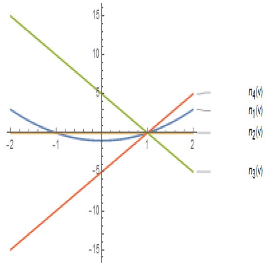
so, since${\mathfrak{n}}_1\left(\mathrm{v}\right)={\mathrm{v}}^2-1,{\mathfrak{n}}_2\left(\mathrm{v}\right)=0,{\mathfrak{n}}_3\left(\mathrm{v}\right)=5(1-\mathrm{v}),{\mathfrak{n}}_4\left(\mathrm{v}\right)=5(\mathrm{v}-1)$(see Figure 1), according to condition (2) we find

$${\eta }^{\prime }\left(\mathrm{v}\right)=({({\mathrm{v}}^2-1)}^2,10({\mathrm{v}}^2-1)(\mathrm{v}-1),10({\mathrm{v}}^2-1)(1-\mathrm{v})).$$

By integrating ${\eta }^{\prime }\left(\mathrm{v}\right),$ we obtain an MPH curve $\eta \left(\mathrm{v}\right)$ of type $(2,0)$ with initial condition $\eta \left(0\right)=(0,0,0)$ as follows:

$$\eta \left(\mathrm{v}\right)=({\displaystyle \frac{1}{5}}{\mathrm{v}}^5-{\displaystyle \frac{2}{3}}{\mathrm{v}}^3+\mathrm{v},{\displaystyle \frac{5}{2}}{\mathrm{v}}^4-{\displaystyle \frac{10}{3}}{\mathrm{v}}^3-5{\mathrm{v}}^2+10\mathrm{v},-{\displaystyle \frac{5}{2}}{\mathrm{v}}^4+{\displaystyle \frac{10}{3}}{\mathrm{v}}^3+5{\mathrm{v}}^2-10\mathrm{v}).$$

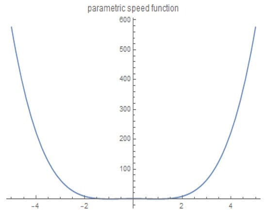
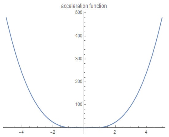
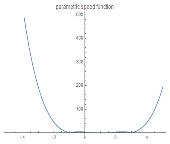
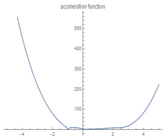
Since $\sigma \left(\mathrm{v}\right)=\left|\mathfrak{W}\left(\mathrm{v}\right)\right|={\mathrm{v}}^4-2{\mathrm{v}}^2+1={({\mathrm{v}}^2-1)}^2\ne 0,$ we have $\mathrm{v}\in \mathbb{R}\setminus \left\{-1,1\right\}$ (For the parametric speed function and acceleration function of the MPH curve of type (2,0), see Figure 2 and Figure 3). Using Definition (3), one can easily compute the ERF $\left\{{\mathsf{\ae }}_1\left(\mathrm{v}\right),{\mathsf{\ae }}_2\left(\mathrm{v}\right),{\mathsf{\ae }}_3\left(\mathrm{v}\right)\right\}$ of $\eta \left(\mathrm{v}\right)$ as follows:

$$\begin{array}{ccc}\hfill {\mathsf{\ae }}_1\left(\mathrm{v}\right)& =& (1,{\displaystyle \frac{10}{\mathrm{v}+1}},-{\displaystyle \frac{10}{\mathrm{v}+1}}),\hfill \\ \hfill {\mathsf{\ae }}_2\left(\mathrm{v}\right)& =& (-{\displaystyle \frac{10}{\mathrm{v}+1}},1-{\displaystyle \frac{50}{{(\mathrm{v}+1)}^2}},{\displaystyle \frac{50}{{(\mathrm{v}+1)}^2}}),\hfill \\ \hfill {\mathsf{\ae }}_3\left(\mathrm{v}\right)& =& (-{\displaystyle \frac{10}{\mathrm{v}+1}},-{\displaystyle \frac{50}{{(\mathrm{v}+1)}^2}},1+{\displaystyle \frac{50}{{(\mathrm{v}+1)}^2}}).\hfill \end{array}$$

Since the MPH curve $\eta \left(\mathrm{v}\right)$ is of type $(2,0),$ its ERF is an RRMF.

CNC tool paths are usually defined by code that interpolates discrete tool positions along linear and circular segments. Geometrically, this method is simple and the tool speed can be easily controlled along the segments. However, this technique can lead to problems with inaccuracies and also increase the data volume. Furthermore, circular and linear segments can only provide continuity of speed, but since the acceleration will always be intermittent, the possible speed of the machine is limited. As a result, the continuity of the speed function and the acceleration function of the curve on which the CNC tool paths are defined increases the tool machining speed.

4.2. MPH Curves of Type (2,1)

A quintic regular spacelike spatial MPH curve $\eta \left(v\right)$ is of type (2,1) iff polynomials ${\tau }_1\left(v\right),{\tau }_2\left(v\right)$ exist where $gcd({\tau }_1\left(v\right),{\tau }_2\left(v\right))$ is constant, ${\tau }_1\left(v\right)+\mathbf{e}{\tau }_2\left(v\right)$ is a linear hyperbolic polynomial and

$$-{\displaystyle \frac{w\left(v\right)}{\sigma \left(v\right)}}={\displaystyle \frac{{\tau }_1\left(v\right){\tau }_2^{\prime }\left(v\right)-{\tau }_1^{\prime }\left(v\right){\tau }_2\left(v\right)}{{\tau }_1^2\left(v\right)-{\tau }_2^2\left(v\right)}}.$$

Since ${\tau }_1\left(v\right)$ or ${\tau }_2\left(v\right)$ is linear and they are relatively prime, by Lemmas (2) and (3), we can take ${\tau }_1\left(v\right)=v-\xi ,{\tau }_2\left(v\right)=\mathfrak{r}$ for $\xi ,\mathfrak{r}\in \mathbb{R}$ with $\mathfrak{r}\ne 0.$ Expanding (14), we obtain

$$\begin{array}{ccc}\hfill {\sigma }_3& =& -2({\gamma }_0+{\beta }_0),{\sigma }_2=\left|C_1\right|+\left|C_2\right|+4{\gamma }_0{\beta }_0,\hfill \\ \hfill {\sigma }_1& =& -2({\gamma }_0\left|C_2\right|+{\beta }_0\left|C_1\right|),{\sigma }_0=\left|C_1\right|\left|C_2\right|.\hfill \end{array}$$

Since

$$\begin{array}{ccc}\hfill \mathfrak{W}\left(v\right)& =& v^2-(C_1+C_2)v+C_1{C}_2\hfill \\ & =& v^2-({\gamma }_0+{\beta }_0)v+{\gamma }_0{\beta }_0+{\gamma }_1{\beta }_1+{\gamma }_2{\beta }_2-{\gamma }_3{\beta }_3\hfill \\ & & +\mathbf{i}(-({\gamma }_1+{\beta }_1)v+{\gamma }_0{\beta }_1+{\gamma }_1{\beta }_0+{\gamma }_2{\beta }_3-{\gamma }_3{\beta }_2)\hfill \\ & & +\mathbf{j}(-({\gamma }_2+{\beta }_2)v+{\gamma }_0{\beta }_2-{\gamma }_1{\beta }_3+{\gamma }_2{\beta }_0+{\gamma }_3{\beta }_1)\hfill \\ & & +\mathbf{k}(-({\gamma }_3+{\beta }_3)v+{\gamma }_0{\beta }_3-{\gamma }_1{\beta }_2+{\gamma }_2{\beta }_1+{\gamma }_3{\beta }_0)\hfill \end{array}$$

and

$${\mathfrak{W}}^{{\prime }^{*}}\left(v\right)=2v-({\gamma }_0+{\beta }_0)+({\gamma }_1+{\beta }_1)\mathbf{i}+({\gamma }_2+{\beta }_2)\mathbf{j}+({\gamma }_3+{\beta }_3)\mathbf{k},$$

by substituting in (13), we have that $w\left(v\right)$ has coefficients

$$\begin{array}{ccc}\hfill w_2& =& -({\gamma }_1+{\beta }_1),\hfill \\ \hfill w_1& =& 2({\gamma }_0{\beta }_1+{\gamma }_1{\beta }_0+{\gamma }_2{\beta }_3-{\gamma }_3{\beta }_2),\hfill \\ \hfill w_0& =& ({\gamma }_1+{\beta }_1)({\gamma }_0{\beta }_0+{\gamma }_1{\beta }_1+{\gamma }_2{\beta }_2-{\gamma }_3{\beta }_3)-({\gamma }_0+{\beta }_0)({\gamma }_0{\beta }_1+{\gamma }_1{\beta }_0+{\gamma }_2{\beta }_3-{\gamma }_3{\beta }_2)\hfill \\ & & -({\gamma }_3+{\beta }_3)({\gamma }_0{\beta }_2-{\gamma }_1{\beta }_3+{\gamma }_2{\beta }_0+{\gamma }_3{\beta }_1)+({\gamma }_2+{\beta }_2)({\gamma }_0{\beta }_3-{\gamma }_1{\beta }_2+{\gamma }_2{\beta }_1+{\gamma }_3{\beta }_0).\hfill \end{array}$$

Thus, the equality

$$-{\displaystyle \frac{w\left(v\right)}{\sigma \left(v\right)}}={\displaystyle \frac{-\mathfrak{r}}{v^2-2\xi v+{\xi }^2-{\mathfrak{r}}^2}}$$

is equivalent to

$$\begin{array}{ccc}\hfill \mathfrak{r}& =& w_2,\hfill \\ \hfill \mathfrak{r}{\sigma }_3& =& w_1-2\xi w_2,\hfill \\ \hfill \mathfrak{r}{\sigma }_2& =& w_2({\xi }^2-{\mathfrak{r}}^2)+w_0-2w_1\xi ,\hfill \\ \hfill \mathfrak{r}{\sigma }_1& =& w_1({\xi }^2-{\mathfrak{r}}^2)-2w_0\xi ,\hfill \\ \hfill \mathfrak{r}{\sigma }_0& =& w_0({\xi }^2-{\mathfrak{r}}^2).\hfill \end{array}$$

(16)

Since $\mathfrak{r}=w_2\ne 0,$ we obtain

$$\xi ={\displaystyle \frac{w_1-w_2{\sigma }_3}{2w_2}},$$

and hence we obtain that curve $\eta \left(v\right)$ is of type (2,1) iff

$$\xi ={\displaystyle \frac{w_1-w_2{\sigma }_3}{2w_2}}\mathrm{and}\mathfrak{r}=w_2,$$

and these values must satisfy the last three equations of system (16). Thus, following theorem is proved.

Theorem 8.

Let $\mathfrak{W}\left(\mathrm{v}\right)=(\mathrm{v}-C_1)(\mathrm{v}-C_2)$ with $C_1={\gamma }_0+{\gamma }_1\mathbf{i}+{\gamma }_2\mathbf{j}+{\gamma }_3\mathbf{k},C_2={\beta }_0+{\beta }_1\mathbf{i}+{\beta }_2\mathbf{j}+{\beta }_3\mathbf{k}\in \tilde{\mathbb{H}}.$ Set $w\left(\mathrm{v}\right)=scal\left(\mathfrak{W}\left(\mathrm{v}\right)i{\mathfrak{W}}^{\prime *}\left(\mathrm{v}\right)\right)=w_2{\mathrm{v}}^2+w_1\mathrm{v}+w_0$ and $\sigma \left(\mathrm{v}\right)=\left|\mathfrak{W}\left(\mathrm{v}\right)\right|={\mathrm{v}}^4+{\sigma }_3{\mathrm{v}}^3+{\sigma }_2{\mathrm{v}}^2+{\sigma }_1\mathrm{v}+{\sigma }_0.$ Then, the regular spacelike spatial MPH curve generated by split quaternion polynomial $\mathfrak{W}\left(\mathrm{v}\right)$ is of type (2,1) iff system

$$\begin{array}{ccc}\hfill \mathfrak{r}{\sigma }_2& =& w_2({\xi }^2-{\mathfrak{r}}^2)+w_0-2w_1\xi ,\hfill \\ \hfill \mathfrak{r}{\sigma }_1& =& w_1({\xi }^2-{\mathfrak{r}}^2)-2w_0\xi ,\hfill \\ \hfill \mathfrak{r}{\sigma }_0& =& w_0({\xi }^2-{\mathfrak{r}}^2)\hfill \end{array}$$

has the solution

$$(\xi ,\mathfrak{r})=({\displaystyle \frac{w_1-w_2{\sigma }_3}{2w_2}},w_2).$$

Example 2.

Let $\mathfrak{W}\left(\mathrm{v}\right)=(\mathrm{v}-1+\mathbf{j}-\mathbf{k})(\mathrm{v}-1-\mathbf{i}-2\mathbf{j}+\mathbf{k})$ be a split quaternion polynomial that defines a regular spacelike spatial MPH quintic curve $\eta \left(\mathrm{v}\right)$. We can easily see that

$$w_0=1,w_1=0,w_2=-1,$$

$${\sigma }_0=-3,{\sigma }_1=4,{\sigma }_2=2,{\sigma }_3=-4,$$

$$\xi =2,\mathfrak{r}=-1$$

and the system of Theorem (8) is verified by the values of $\xi ,\mathfrak{r}.$ Thus, $\mathfrak{W}\left(\mathrm{v}\right)$ defines an MPH curve of type (2,1). One can easily see that

$$\mathfrak{W}\left(\mathrm{v}\right)=({\mathrm{v}}^2-2\mathrm{v})-\mathbf{i}\mathrm{v}+\mathbf{j}(-\mathrm{v}+2)-\mathbf{k},$$

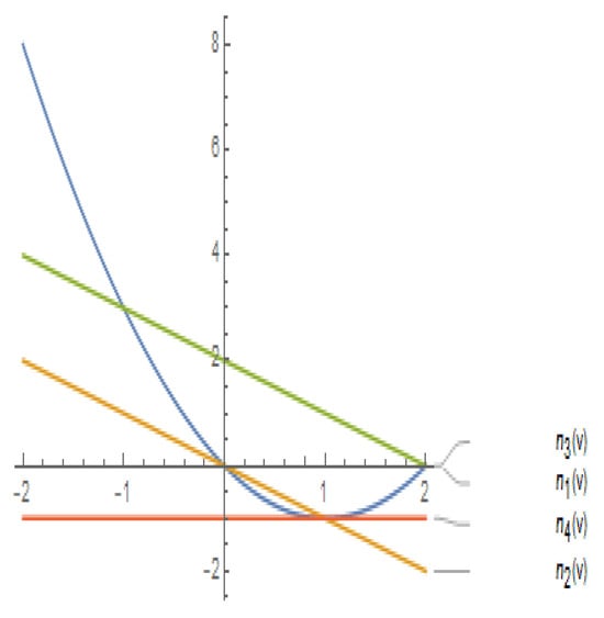
so, since${\mathfrak{n}}_1\left(\mathrm{v}\right)={\mathrm{v}}^2-2\mathrm{v},{\mathfrak{n}}_2\left(\mathrm{v}\right)=-\mathrm{v},{\mathfrak{n}}_3\left(\mathrm{v}\right)=-\mathrm{v}+2,{\mathfrak{n}}_4\left(\mathrm{v}\right)=-1$ (see Figure 4), according to condition (2) we find

$${\eta }^{\prime }\left(\mathrm{v}\right)=({\mathrm{v}}^4-4{\mathrm{v}}^3+4{\mathrm{v}}^2-4\mathrm{v}+3,-4{\mathrm{v}}^2+8\mathrm{v},-2{\mathrm{v}}^3+8{\mathrm{v}}^2-10\mathrm{v}).$$

By integrating ${\eta }^{\prime }\left(\mathrm{v}\right),$ we obtain an MPH curve $\eta \left(\mathrm{v}\right)$ of type (2,1) with initial condition $\eta \left(0\right)=(0,0,0)$ as follows:

$$\eta \left(\mathrm{v}\right)=({\displaystyle \frac{1}{5}}{\mathrm{v}}^5-{\mathrm{v}}^4+{\displaystyle \frac{4}{3}}{\mathrm{v}}^3-2{\mathrm{v}}^2+3\mathrm{v},-{\displaystyle \frac{4}{3}}{\mathrm{v}}^3+4{\mathrm{v}}^2,-{\displaystyle \frac{1}{2}}{\mathrm{v}}^4+{\displaystyle \frac{8}{3}}{\mathrm{v}}^3-5{\mathrm{v}}^2).$$

Since $\sigma \left(\mathrm{v}\right)=\left|\mathfrak{W}\left(\mathrm{v}\right)\right|={\mathrm{v}}^4-4{\mathrm{v}}^3+2{\mathrm{v}}^2+4\mathrm{v}-3\ne 0,$ we have $\mathrm{v}\in \mathbb{R}\setminus \left\{-1,1,3\right\}$ (For the parametric speed function and acceleration function of the MPH curve of type (2,0), see Figure 5 and Figure 6). Using Definition (3), one can easily compute the ERF $\left\{{\mathsf{\ae }}_1\left(\mathrm{v}\right),{\mathsf{\ae }}_2\left(\mathrm{v}\right),{\mathsf{\ae }}_3\left(\mathrm{v}\right)\right\}$ of $\eta \left(\mathrm{v}\right)$ as follows:

$$\begin{array}{ccc}\hfill {\mathsf{\ae }}_1\left(\mathrm{v}\right)& =& {\displaystyle \frac{({\mathrm{v}}^4-4{\mathrm{v}}^3+4{\mathrm{v}}^2-4\mathrm{v}+3,-4{\mathrm{v}}^2+8\mathrm{v},-2{\mathrm{v}}^3+8{\mathrm{v}}^2-10\mathrm{v})}{{\mathrm{v}}^4-4{\mathrm{v}}^3+2{\mathrm{v}}^2+4\mathrm{v}-3}},\hfill \\ \hfill {\mathsf{\ae }}_2\left(\mathrm{v}\right)& =& {\displaystyle \frac{(0,{\mathrm{v}}^4-4{\mathrm{v}}^3+4{\mathrm{v}}^2+4\mathrm{v}-5,2{\mathrm{v}}^3-4{\mathrm{v}}^2-2\mathrm{v}+4)}{{\mathrm{v}}^4-4{\mathrm{v}}^3+2{\mathrm{v}}^2+4\mathrm{v}-3}},\hfill \\ \hfill {\mathsf{\ae }}_3\left(\mathrm{v}\right)& =& {\displaystyle \frac{(-2{\mathrm{v}}^3+8{\mathrm{v}}^2-6\mathrm{v},2{\mathrm{v}}^3-4{\mathrm{v}}^2+2\mathrm{v}-4,{\mathrm{v}}^4-4{\mathrm{v}}^3+6{\mathrm{v}}^2-4\mathrm{v}+5)}{{\mathrm{v}}^4-4{\mathrm{v}}^3+2{\mathrm{v}}^2+4\mathrm{v}-3}}.\hfill \end{array}$$

Since ${\tau }_1\left(\mathrm{v}\right)=\mathrm{v}-2$ and ${\tau }_2\left(\mathrm{v}\right)=-1$, from Theorem (2), a RRMF $\left\{{\mathbf{f}}_1\left(\mathrm{v}\right),{\mathbf{f}}_2\left(\mathrm{v}\right),{\mathbf{f}}_3\left(\mathrm{v}\right)\right\}$ of $\eta \left(\mathrm{v}\right)$ is obtained as follows,

$$\begin{array}{ccc}\hfill {\mathbf{f}}_1\left(\mathrm{v}\right)& =& {\mathsf{\ae }}_1\left(\mathrm{v}\right),\hfill \\ \hfill {\mathbf{f}}_2\left(\mathrm{v}\right)& =& {\displaystyle \frac{{\mathrm{v}}^2-4\mathrm{v}+5}{{\mathrm{v}}^2-4\mathrm{v}+3}}{\mathsf{\ae }}_2\left(\mathrm{v}\right)+{\displaystyle \frac{-2\mathrm{v}+4}{{\mathrm{v}}^2-4\mathrm{v}+3}}{\mathsf{\ae }}_3\left(\mathrm{v}\right),\hfill \\ \hfill {\mathbf{f}}_3\left(\mathrm{v}\right)& =& {\displaystyle \frac{-2\mathrm{v}+4}{{\mathrm{v}}^2-4\mathrm{v}+3}}{\mathsf{\ae }}_2\left(\mathrm{v}\right)+{\displaystyle \frac{{\mathrm{v}}^2-4\mathrm{v}+5}{{\mathrm{v}}^2-4\mathrm{v}+3}}{\mathsf{\ae }}_3\left(\mathrm{v}\right).\hfill \end{array}$$

5. Applications

In fixed axisymmetric spacetimes, Fermi–Walker-transported frames are immensely useful in understanding the characteristics of timelike circular orbits and assist in visualizing the geometry of this family of orbits. Additionally, the Fermi–Walker derivative is significant to understand the geodesics. For example, to find what kind of curves in ${\mathbb{R}}^n$ are geodesics, one can take into account the connection of the Fermi–Walker derivative. If $\alpha$ is a curve in ${\mathbb{R}}^n$, T is its tangent vector field and $\tilde{\nabla }$ is the Fermi–Walker derivative, then ${\tilde{\nabla }}_{T}T=0$ holds for every line in ${\mathbb{R}}^n$ [38]. For the applications of the Fermi–Walker derivative and parallelism in physics, one can see the references [39,40,41].

In this section, the Fermi–Walker derivative is calculated with respect to the ERF defined for a regular spacelike spatial MPH curve in Definition (3). The Fermi–Walker derivative and parallelism defined with respect to the ERF for MPH curves are intended to be used in modeling the motions along these curves. For this purpose, the solution of the homogeneous normal linear differential equation system that must be satisfied for a vector field to be parallel in a Fermi–Walker sense with respect to the ERF along a regular spacelike spatial MPH curve is obtained.

Theorem 9.

Let $\eta \left(\mathrm{v}\right)$ be a regular spacelike spatial MPH curve generated by split quaternion polynomial $\mathfrak{W}\left(\mathrm{v}\right)={\mathfrak{n}}_1\left(\mathrm{v}\right)+\mathbf{i}{\mathfrak{n}}_2\left(\mathrm{v}\right)+\mathbf{j}{\mathfrak{n}}_3\left(\mathrm{v}\right)+\mathbf{k}{\mathfrak{n}}_4\left(\mathrm{v}\right)$. Derivation formulas for the ERF $\{{\mathsf{\ae }}_1\left(\mathrm{v}\right),{\mathsf{\ae }}_2\left(\mathrm{v}\right),$${\mathsf{\ae }}_3\left(\mathrm{v}\right)\}$ of $\eta \left(\mathrm{v}\right)$ are as follows:

$$\left[\begin{array}{c}{\mathsf{\ae }}_1^{\prime }\left(v\right)\\ {\mathsf{\ae }}_2^{\prime }\left(v\right)\\ {\mathsf{\ae }}_3^{\prime }\left(v\right)\end{array}\right]=\left[\begin{array}{ccc}0& {\pi }_1\left(v\right)& -{\pi }_2\left(v\right)\\ -{\pi }_1\left(v\right)& 0& {\pi }_3\left(v\right)\\ {\pi }_2\left(v\right)& -{\pi }_3\left(v\right)& 0\end{array}\right]\left[\begin{array}{c}{\mathsf{\ae }}_1\left(v\right)\\ {\mathsf{\ae }}_2\left(v\right)\\ {\mathsf{\ae }}_3\left(v\right)\end{array}\right],$$

where

$$\begin{array}{ccc}\hfill {\pi }_1\left(v\right)& =& {\displaystyle \frac{2({\mathfrak{n}}_1\left(v\right){\mathfrak{n}}_4^{\prime }\left(v\right)-{\mathfrak{n}}_4\left(v\right){\mathfrak{n}}_1^{\prime }\left(v\right)+{\mathfrak{n}}_2\left(v\right){\mathfrak{n}}_3^{\prime }\left(v\right)-{\mathfrak{n}}_3\left(v\right){\mathfrak{n}}_2^{\prime }\left(v\right)}{\left|\mathfrak{W}\left(v\right)\right|}},\hfill \\ \hfill {\pi }_2\left(v\right)& =& {\displaystyle \frac{2({\mathfrak{n}}_1\left(v\right){\mathfrak{n}}_3^{\prime }\left(v\right)-{\mathfrak{n}}_3\left(v\right){\mathfrak{n}}_1^{\prime }\left(v\right)-{\mathfrak{n}}_4\left(v\right){\mathfrak{n}}_2^{\prime }\left(v\right)+{\mathfrak{n}}_2\left(v\right){\mathfrak{n}}_4^{\prime }\left(v\right)}{\left|\mathfrak{W}\left(v\right)\right|}},\hfill \\ \hfill {\pi }_3\left(v\right)& =& {\displaystyle \frac{2({\mathfrak{n}}_1\left(v\right){\mathfrak{n}}_2^{\prime }\left(v\right)-{\mathfrak{n}}_2\left(v\right){\mathfrak{n}}_1^{\prime }\left(v\right)+{\mathfrak{n}}_4\left(v\right){\mathfrak{n}}_3^{\prime }\left(v\right)-{\mathfrak{n}}_3\left(v\right){\mathfrak{n}}_4^{\prime }\left(v\right)}{\left|\mathfrak{W}\left(v\right)\right|}}.\hfill \end{array}$$

Proof. 

One can obtain the result by direct calculations. □

Definition 6.

Let η be a regular spacelike spatial MPH curve and X be a vector field defined along curve $\eta .$ The Fermi–Walker derivative of X with respect to the ERF along η is defined as

$${\tilde{\nabla }}_{{\mathsf{\ae }}_1}X={\nabla }_{{\mathsf{\ae }}_1}X-{〈{\mathsf{\ae }}_1,X〉}_L{\nabla }_{{\mathsf{\ae }}_1}{\mathsf{\ae }}_1+{〈{\nabla }_{{\mathsf{\ae }}_1}{\mathsf{\ae }}_1,X〉}_L{\mathsf{\ae }}_1.$$

Definition 7.

If the Fermi–Walker derivative of a vector field X defined along a regular spacelike spatial MPH curve η with respect to the ERF is zero, i.e., ${\tilde{\nabla }}_{{\mathsf{\ae }}_1}X=0,$ then X is said to be parallel in a Fermi–Walker sense with respect to the ERF along $\eta .$

Definition 8.

Let $A,B,C$ be orthogonal vector fields in ${\mathbb{R}}_1^3.$ If the Fermi–Walker derivatives of these vector fields along a regular spacelike spatial MPH curve with respect to ERF are zero, i.e.,

$$\begin{array}{ccc}\hfill {\tilde{\nabla }}_{{\mathsf{\ae }}_1}A& =& 0,\hfill \\ \hfill {\tilde{\nabla }}_{{\mathsf{\ae }}_1}B& =& 0,\hfill \\ \hfill {\tilde{\nabla }}_{{\mathsf{\ae }}_1}C& =& 0,\hfill \end{array}$$

then $\left\{A,B,C\right\}$ is called a non-rotating frame along the curve.

Theorem 10.

The Fermi–Walker derivative of a vector field X defined along a regular spacelike spatial MPH curve with respect to the ERF is

$${\tilde{\nabla }}_{{\mathsf{\ae }}_1}X={\nabla }_{{\mathsf{\ae }}_1}X+({\pi }_2{\mathsf{\ae }}_2-{\pi }_1{\mathsf{\ae }}_3){\times }_{L}X.$$

Proof. 

One can obtain the result by using Theorem (9) and well-known identity $\left(A{\times }_{L}B\right){\times }_{L}C=-{〈A,C〉}_{L}B+{〈B,C〉}_{L}A$ satisfied by vectors $A,B,C$ in ${\mathbb{R}}_1^3.$ □

Corollary 1.

The ERF of a regular spacelike spatial MPH curve is not non-rotating.

Proof. 

Using Theorem (10), we obtain

$$\begin{array}{ccc}\hfill {\tilde{\nabla }}_{{\mathsf{\ae }}_1}{\mathsf{\ae }}_1& =& 0,\hfill \\ \hfill {\tilde{\nabla }}_{{\mathsf{\ae }}_1}{\mathsf{\ae }}_2& =& {\pi }_3{\mathsf{\ae }}_3,\hfill \\ \hfill {\tilde{\nabla }}_{{\mathsf{\ae }}_1}{\mathsf{\ae }}_3& =& 2{\pi }_2{\mathsf{\ae }}_1-{\pi }_3{\mathsf{\ae }}_2.\hfill \end{array}$$

Therefore, vector fields ${\mathsf{\ae }}_2$ and ${\mathsf{\ae }}_3$ are not parallel in the Fermi–Walker sense. Thus, the ERF is not non-rotating. □

Corollary 2.

The Fermi–Walker derivative of a vector field X defined along a regular spacelike spatial MPH curve η with respect to the ERF coincides with standard derivative iff $X=\lambda ({\pi }_2{\mathsf{\ae }}_2-{\pi }_1{\mathsf{\ae }}_3),$ where $\lambda \in \mathbb{R}.$

Proof. 

${\tilde{\nabla }}_{{\mathsf{\ae }}_1}X={\nabla }_{{\mathsf{\ae }}_1}X$⇔$({\pi }_2{\mathsf{\ae }}_2-{\pi }_1{\mathsf{\ae }}_3){\times }_{L}X=0$⇔$X=\lambda ({\pi }_2{\mathsf{\ae }}_2-{\pi }_1{\mathsf{\ae }}_3).$□

Definition 9.

The Darboux vector of a regular spacelike spatial MPH curve with respect to the ERF is defined as

$$W=-{\pi }_3{\mathsf{\ae }}_1\left(\mathrm{v}\right)-{\pi }_2{\mathsf{\ae }}_2\left(\mathrm{v}\right)+{\pi }_1{\mathsf{\ae }}_3\left(\mathrm{v}\right).$$

Theorem 11.

The Fermi–Walker derivative of a vector field X defined along a regular spacelike spatial MPH curve with respect to the ERF is

$${\tilde{\nabla }}_{{\mathsf{\ae }}_1}X={\nabla }_{{\mathsf{\ae }}_1}X+X{\times }_{L}W+{\pi }_3\left(X{\times }_L{\mathsf{\ae }}_1\right).$$

Proof. 

One can obtain the result by direct calculations using Theorem (10). □

Theorem 12.

Let ${\lambda }_1,{\lambda }_2,{\lambda }_3$ be real-valued continuously differentiable functions of parameter v and $X={\lambda }_1{\mathsf{\ae }}_1\left(\mathrm{v}\right)+{\lambda }_2{\mathsf{\ae }}_2\left(\mathrm{v}\right)+{\lambda }_3{\mathsf{\ae }}_3\left(\mathrm{v}\right)$ be a vector field defined along a regular spacelike spatial MPH curve. Then, X is parallel in a Fermi–Walker sense with respect to the ERF along the curve iff

$$\begin{array}{ccc}\hfill {\lambda }_1& =& -2{\int }_{{\mathrm{v}}_0}^{\mathrm{v}}{\pi }_2\left(\mathrm{v}\right){\lambda }_3\left(\mathrm{v}\right)d\mathrm{v},\hfill \\ \hfill {\lambda }_2& =& a_{1}sin{\int }_{{\mathrm{v}}_0}^{\mathrm{v}}{\pi }_3\left(\mathrm{v}\right)d\mathrm{v}+a_{2}cos{\int }_{{\mathrm{v}}_0}^{\mathrm{v}}{\pi }_3\left(\mathrm{v}\right)d\mathrm{v},\hfill \\ \hfill {\lambda }_3& =& a_{1}cos{\int }_{{\mathrm{v}}_0}^{\mathrm{v}}{\pi }_3\left(\mathrm{v}\right)d\mathrm{v}+a_{2}sin{\int }_{{\mathrm{v}}_0}^{\mathrm{v}}{\pi }_3\left(\mathrm{v}\right)d\mathrm{v},\hfill \end{array}$$

(17)

where $a_1,a_2$ are arbitrary real constants.

Proof. 

One can obtain the result by using Theorem (11) and the definition of Fermi–Walker parallelism. □

Example 3.

Let

$$\eta \left(\mathrm{v}\right)=({\displaystyle \frac{1}{5}}{\mathrm{v}}^5-{\displaystyle \frac{2}{3}}{\mathrm{v}}^3+\mathrm{v},{\displaystyle \frac{5}{2}}{\mathrm{v}}^4-{\displaystyle \frac{10}{3}}{\mathrm{v}}^3-5{\mathrm{v}}^2+10\mathrm{v},-{\displaystyle \frac{5}{2}}{\mathrm{v}}^4+{\displaystyle \frac{10}{3}}{\mathrm{v}}^3+5{\mathrm{v}}^2-10\mathrm{v})$$

be the quintic regular spacelike spatial MPH curve constructed in Example (1). This curve is generated by split quaternion polynomial $\mathfrak{W}\left(\mathrm{v}\right)={\mathfrak{n}}_1\left(\mathrm{v}\right)+\mathbf{i}{\mathfrak{n}}_2\left(\mathrm{v}\right)+\mathbf{j}{\mathfrak{n}}_3\left(\mathrm{v}\right)+\mathbf{k}{\mathfrak{n}}_4\left(\mathrm{v}\right),$ where ${\mathfrak{n}}_1\left(\mathrm{v}\right)={\mathrm{v}}^2-1,$${\mathfrak{n}}_2\left(\mathrm{v}\right)=0,$${\mathfrak{n}}_3\left(\mathrm{v}\right)=5(1-\mathrm{v}),{\mathfrak{n}}_4\left(\mathrm{v}\right)=5(\mathrm{v}-1).$ On the other hand, the ERF of curve $\eta \left(\mathrm{v}\right)$ is

$$\begin{array}{ccc}\hfill {\mathsf{\ae }}_1\left(\mathrm{v}\right)& =& (1,{\displaystyle \frac{10}{\mathrm{v}+1}},-{\displaystyle \frac{10}{\mathrm{v}+1}}),\hfill \\ \hfill {\mathsf{\ae }}_2\left(\mathrm{v}\right)& =& (-{\displaystyle \frac{10}{\mathrm{v}+1}},1-{\displaystyle \frac{50}{{(\mathrm{v}+1)}^2}},{\displaystyle \frac{50}{{(\mathrm{v}+1)}^2}}),\hfill \\ \hfill {\mathsf{\ae }}_3\left(\mathrm{v}\right)& =& (-{\displaystyle \frac{10}{\mathrm{v}+1}},-{\displaystyle \frac{50}{{(\mathrm{v}+1)}^2}},1+{\displaystyle \frac{50}{{(\mathrm{v}+1)}^2}}),\hfill \end{array}$$

where $\mathrm{v}\ne \pm 1.$ Thus, we find ${\pi }_2\left(\mathrm{v}\right)=-{\displaystyle \frac{10}{\mathrm{v}+1}}$ and ${\pi }_3\left(\mathrm{v}\right)=0.$ So, we obtain vector field $X={\lambda }_1{\mathsf{\ae }}_1\left(\mathrm{v}\right)+{\lambda }_2{\mathsf{\ae }}_2\left(\mathrm{v}\right)+{\lambda }_3{\mathsf{\ae }}_3\left(\mathrm{v}\right)$ defined along curve $\eta \left(\mathrm{v}\right)$ is parallel in a Fermi–Walker sense with respect to the ERF, where for $a_1,a_2\in \mathbb{R}$

$$\begin{array}{ccc}\hfill {\lambda }_1\left(\mathrm{v}\right)& =& 20a_{1}ln\left|\mathrm{v}+1\right|,\hfill \\ \hfill {\lambda }_2\left(\mathrm{v}\right)& =& a_2,\hfill \\ \hfill {\lambda }_3\left(\mathrm{v}\right)& =& a_1.\hfill \end{array}$$

Indeed, since ${\pi }_2\left(\mathrm{v}\right)=-{\displaystyle \frac{10}{\mathrm{v}+1}}$ and ${\pi }_3\left(\mathrm{v}\right)=0,$ if we choose ${\lambda }_2\left(\mathrm{v}\right)=a_2,$${\lambda }_3\left(\mathrm{v}\right)=a_1$ and ${\mathrm{v}}_0=0,$ from Theorem (12), we obtain

$$\begin{array}{ccc}\hfill {\lambda }_1& =& -2{\int }_0^{\mathrm{v}}{\pi }_2\left(\mathrm{v}\right){\lambda }_3\left(\mathrm{v}\right)d\mathrm{v}\hfill \\ & =& 20a_1{\int }_0^{\mathrm{v}}{\displaystyle \frac{1}{\mathrm{v}+1}}d\mathrm{v}\hfill \\ & =& 20a_{1}ln\left|\mathrm{v}+1\right|.\hfill \end{array}$$

Thus, the parallelism condition given by the system of differential Equation (17) is satisfied.

6. Conclusions

Leaving null curves aside, we study regular spacelike spatial MPH curves and their representations with symbolic computation methods. As an alternative to the split quaternion representation, we give a new characterization of spatial MPH curves in terms of hyperbolic polynomials using a Minkowski–Hopf map. We show that spatial MPH curves can be obtained from a hyperbolic polynomial couple using Minkowski–Hopf map. Then, we prove necessary and sufficient conditions for an MPH curve to be planar and to be a straight line.

This paper aimed to characterize spatial MPH curves with RRMFs. In order to obtain the necessary and sufficient condition for a spatial MPH curve to have a RRMF, we define the ERF for this kind of curve. Then, we prove that this condition is the existence of polynomials ${\tau }_1\left(v\right),{\tau }_2\left(v\right)$ such that $gcd({\tau }_1\left(v\right),{\tau }_2\left(v\right))$ is constant and

$${\displaystyle \frac{{\mathfrak{n}}_1{\mathfrak{n}}_2^{\prime }-{\mathfrak{n}}_1^{\prime }{\mathfrak{n}}_2-{\mathfrak{n}}_3{\mathfrak{n}}_4^{\prime }+{\mathfrak{n}}_3^{\prime }{\mathfrak{n}}_4}{{\mathfrak{n}}_1^2-{\mathfrak{n}}_2^2-{\mathfrak{n}}_3^2+{\mathfrak{n}}_4^2}}={\displaystyle \frac{{\tau }_1{\tau }_2^{\prime }-{\tau }_1^{\prime }{\tau }_2}{{\tau }_1^2-{\tau }_2^2}},$$

when $\mathfrak{W}\left(v\right)={\mathfrak{n}}_1\left(v\right)+\mathbf{i}{\mathfrak{n}}_2\left(v\right)+\mathbf{j}{\mathfrak{n}}_3\left(v\right)+\mathbf{k}{\mathfrak{n}}_4\left(v\right)$ is a split quaternion polynomial by which the spatial MPH curve is represented. In order to define the concept of type $(n,m)$ curve for spatial MPH curves, we have to show that the degrees of these polynomials ${\tau }_1\left(v\right),{\tau }_2\left(v\right)$ are uniquely determined. Therefore, we prove a theorem that shows this uniqueness. Thus, we define the concept of type $(n,m)$ curves for spatial MPH curves. This concept is a useful tool to characterize spatial MPH curves. We characterize quintic spatial MPH curves of type $(2,0)$ and $(2,1),$ when the quadratic split quaternion polynomial that generates the curve is in normal form and admits a factorization. We give illustrative examples for these types of quintic spatial MPH curves.

References

- Farouki, R.T.; Sakkalis, T. Pythagorean Hodographs. IBM J. Res. Dev. 1990, 34, 736–752. [Google Scholar] [CrossRef]
- Choi, H.I.; Han, C.Y. Euler-Rodrigues Frames on Spatial Pythagorean-Hodograph Curves. Comput. Aided Geom. Des. 2002, 19, 603–620. [Google Scholar] [CrossRef]
- Han, C.Y. Nonexistence of Rational Rotation-Minimizing Frames on Cubic Curves. Comput. Aided Geom. Des. 2008, 25, 298–304. [Google Scholar] [CrossRef]
- Dospra, P. Quaternion Polynomials and Rational Rotation-Minimizing Frame Curves. Ph.D. Thesis, Agricultural University of Athens, Athens, Greece, 2015. [Google Scholar]
- Moon, H.P. Minkowski Pythagorean Hodographs. Comput. Aided Geom. Des. 1999, 16, 739–753. [Google Scholar] [CrossRef]
- Choi, H.I.; Lee, D.S.; Moon, H.P. Spin Representation and Rational Parameterization of Curves and Surfaces. Adv. Comput. Math. 2002, 17, 5–48. [Google Scholar] [CrossRef]
- Ramis, Ç. PH Curves and Applications. Master’s Thesis, Ankara University, Ankara, Turkey, 2013. [Google Scholar]
- Kosinka, J.; Lávička, M. On Rational Minkowski Pythagorean Hodograph Curves. Comput. Aided Geom. Des. 2010, 27, 514–524. [Google Scholar] [CrossRef]
- Farouki, R.T. Pythagorean-Hodograph Curves; Springer: Berlin/Heidelberg, Germany, 2008. [Google Scholar]
- Tsai, M.S.; Nien, H.W.; Yau, H.T. Development of an integrated look-ahead dynamics-based NURBS interpolator for high precision machinery. Comput.-Aided Des. 2008, 40, 554–566. [Google Scholar] [CrossRef]
- Farouki, R.T.; Sakkalis, T. Pythagorean-Hodograph Space Curves. Adv. Comput. Math. 1994, 2, 41–66. [Google Scholar] [CrossRef]
- Farouki, R.T. Quaternion and Hopf map characterizations for the existence of rational rotation-minimizing frames on quintic space curves. Adv. Comput. Math. 2010, 33, 331–348. [Google Scholar] [CrossRef]
- Tsai, Y.F.; Farouki, R.T.; Feldman, B. Performance analysis of CNC interpolators for time-dependent feedrates along PH curves. Comput. Aided Geom. Des. 2001, 18, 245–265. [Google Scholar] [CrossRef]
- Singh Bains, P.; Sidhu, S.S.; Payal, H.S. Investigation of magnetic field-assisted EDM of composites. Mater. Manuf. Process. 2018, 33, 670–675. [Google Scholar] [CrossRef]
- Fu, H.; Lei, T.; Su, M.; Yan, T. Complexity Dynamic Analysis of Fractional-order Permanent Magnet Synchronous Motor in CNC Machine Tool. J. Phys. Conf. Ser. Iop Publ. 2021, 1861, 012107. [Google Scholar]
- Chen, C.K.; Li, Y.C. Intelligent real-time monitoring of Computer Numerical Control tool wear based on a fractional-order chaotic self-synchronization system. J. Low Freq. Noise Vib. Act. Control 2019, 38, 1555–1566. [Google Scholar] [CrossRef]
- Chen, C.K.; Li, Y.C. Machine chattering identification based on the fractional-order chaotic synchronization dynamic error. Int. J. Adv. Manuf. Technol. 2019, 100, 907–915. [Google Scholar] [CrossRef]
- Nittler, K.M.; Farouki, R.T. Efficient high-speed cornering motions based on continuously-variable feedrates. II. Implementation and performance analysis. Int. J. Adv. Manuf. Technol. 2019, 88, 159–174. [Google Scholar] [CrossRef]
- Arrizabalaga, J.; Ryll, M. Spatial motion planning with pythagorean hodograph curves. In Proceedings of the 61st Conference on Decision and Control (CDC), Cancun, Mexico, 6–9 December 2022. [Google Scholar]
- Bezawada, H.; Woods, C.; Vikas, V. Shape estimation of soft manipulators using piecewise continuous Pythagorean-hodograph curves. In Proceedings of the 2022 American Control Conference (ACC), Atlanta, GA, USA, 8–10 June 2022. [Google Scholar]
- Deaf, A.A.; Eid, A.H.; Elserafi, K. Optimized UAVs’ Collision-free 2D Path Planning Based on Quintic Pythagorean Hodograph Curves. In Proceedings of the 14th International Conference on Electrical Engineering (ICEENG), Cairo, Egypt, 21–23 May 2024. [Google Scholar]
- Farouki, R.T. Partition of the space of planar quintic Pythagorean-hodograph curves. Comput. Aided Geom. Des. 2023, 106, 102242. [Google Scholar] [CrossRef]
- Farouki, R.T.; Pelosi, F.; Sampoli, M.L. Construction of planar quintic Pythagorean-hodograph curves by control-polygon constraints. Comput. Aided Geom. Des. 2023, 103, 102192. [Google Scholar] [CrossRef]
- Hormann, K.; Romani, L.; Viscardi, A. New algebraic and geometric characterizations of planar quintic Pythagorean-hodograph curves. Comput. Aided Geom. Des. 2024, 108, 102256. [Google Scholar] [CrossRef]
- Li, Y. Characteristics of planar sextic indirect-PH curves. AIMS Math. 2024, 9, 2215–2231. [Google Scholar] [CrossRef]
- Peng, F.; Pang, J.; Pan, Y. Global Optimization Method to Comprise Rotation-Minimizing Euler-Rodrigues Frames of Pythagorean-Hodograph Curve. J. Appl. Math. Phys. 2023, 11, 1250–1262. [Google Scholar] [CrossRef]
- Schröcker, H.P.; Šír, Z. Partial fraction decomposition for rational Pythagorean hodograph curves. J. Comput. Appl. Math. 2023, 428, 115196. [Google Scholar] [CrossRef]
- Singh, I.; Amara, Y.; Melingui, A.; Mani Pathak, P.; Merzouki, R. Modeling of continuum manipulators using pythagorean hodograph curves. Soft Robot. 2018, 5, 425–442. [Google Scholar] [CrossRef] [PubMed]
- Wang, X.Y.; Shen, L.Y.; Yuan, C.M.; Pérez-Díaz, S. On G2 approximation of planar algebraic curves under certified error control by quintic Pythagorean-hodograph splines. Comput. Aided Geom. Des. 2024, 113, 102374. [Google Scholar] [CrossRef]
- Yazla, A.; Sarıaydın, M.T. Double and Type (3, 0) Minkowski Pythagorean Hodograph Curves. Bitlis Eren Univ. Sci. 2022, 11, 660–665. [Google Scholar] [CrossRef]
- López, R. Differential Geometry of Curves and Surfaces in Lorentz-Minkowski Space. Int. Electron. J. Geom. 2014, 7, 44–107. [Google Scholar] [CrossRef]
- O’Neill, B. Semi-Riemannian Geometry with Applications to Relativity; Academic Press: Cambridge, MA, USA, 1983. [Google Scholar]
- Catoni, F.; Boccaletti, D.; Cannata, R.; Catoni, V.; Zampetti, P. Geometry of Minkowski Space-Time; Springer: Berlin/Heidelberg, Germany, 2011. [Google Scholar]
- Inoguchi, J.I. Timelike Surfaces of Constant Mean Curvature in Minkowski 3-Space. Tokyo J. Math. 1998, 21, 141–152. [Google Scholar] [CrossRef]
- Cockle, J. On systems of algebra involving more than one imaginary. Philos. Mag. 1849, 35, 434–435. [Google Scholar]
- Bishop, R.L. There is more than one way to frame a curve. Am. Math. Mon. 1975, 82, 246–251. [Google Scholar] [CrossRef]
- Scharler, D.F.; Siegele, J.; Schröcker, H.P. Quadratic split quaternion polynomials: Factorization and geometry. Adv. Appl. Clifford Algebr. 2020, 30, 1–23. [Google Scholar] [CrossRef]
- Karakuş, F.; Yayli, Y. On the Fermi-Walker derivative and non-rotating frame. Int. J. Geom. Mod. Phys. 2012, 9, 1250066. [Google Scholar] [CrossRef]
- Ogrenmis, M. A generalization of the optical quantum model using fractional normalization and recursion. Opt. Quantum Electron. 2024, 56, 1024. [Google Scholar] [CrossRef]
- Özdemir, Z.; Ndiaye, A. Propagation of polarized light and electromagnetic curves in the optical fiber in Walker 3-Manifolds. Facta Univ. Ser. Math. Inform. 2023, 38, 713–730. [Google Scholar] [CrossRef]
- Sariaydin, M.T. A Conjugate Linearly Polarized Light Wave Along an Optical Fiber with the Berry Phase Model and Its Magnetic Trajectories According to the Conjugate Frame. Symmetry 2024, 16, 1518. [Google Scholar] [CrossRef]
Disclaimer/Publisher’s Note: The statements, opinions and data contained in all publications are solely those of the individual author(s) and contributor(s) and not of MDPI and/or the editor(s). MDPI and/or the editor(s) disclaim responsibility for any injury to people or property resulting from any ideas, methods, instructions or products referred to in the content. |
© 2024 by the authors. Licensee MDPI, Basel, Switzerland. This article is an open access article distributed under the terms and conditions of the Creative Commons Attribution (CC BY) license (https://creativecommons.org/licenses/by/4.0/).