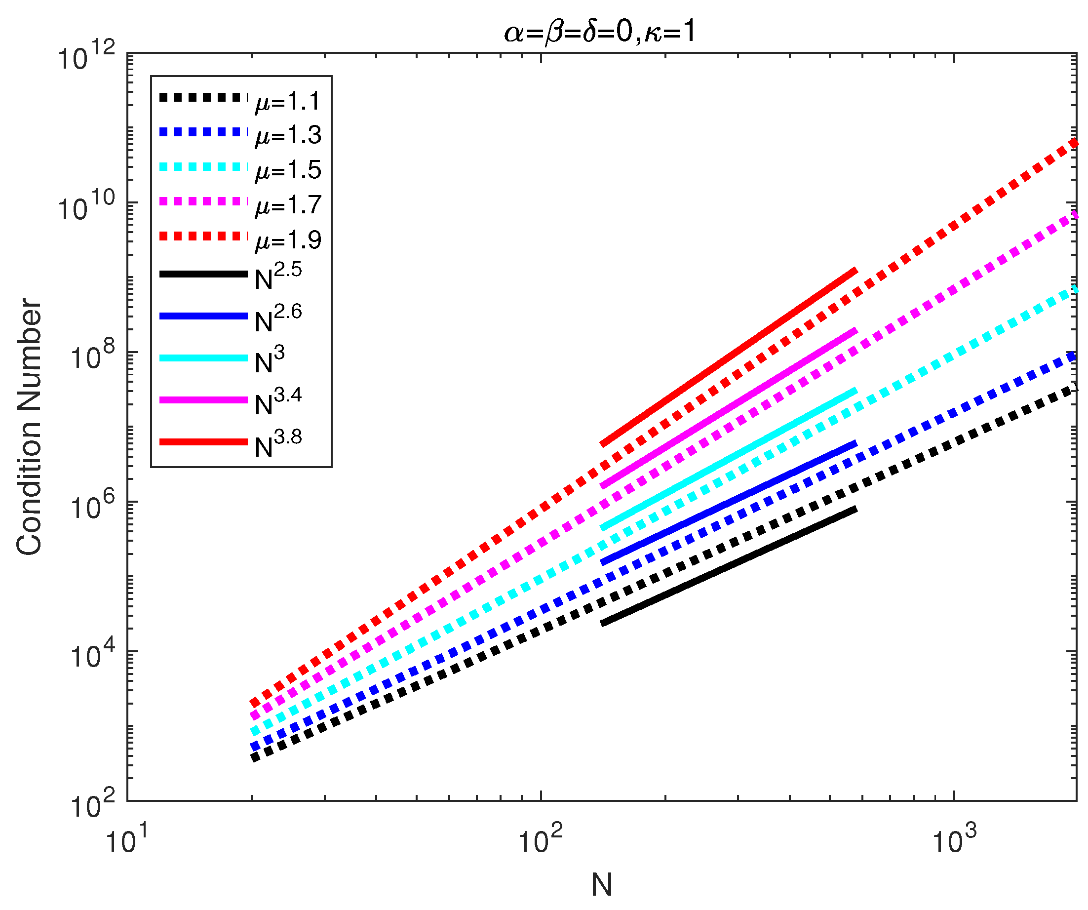
Figure 1.
Condition number of DMLTCD with .
Figure 1.
Condition number of DMLTCD with .
Figure 2.
Condition number of DMLTCD with .
Figure 2.
Condition number of DMLTCD with .
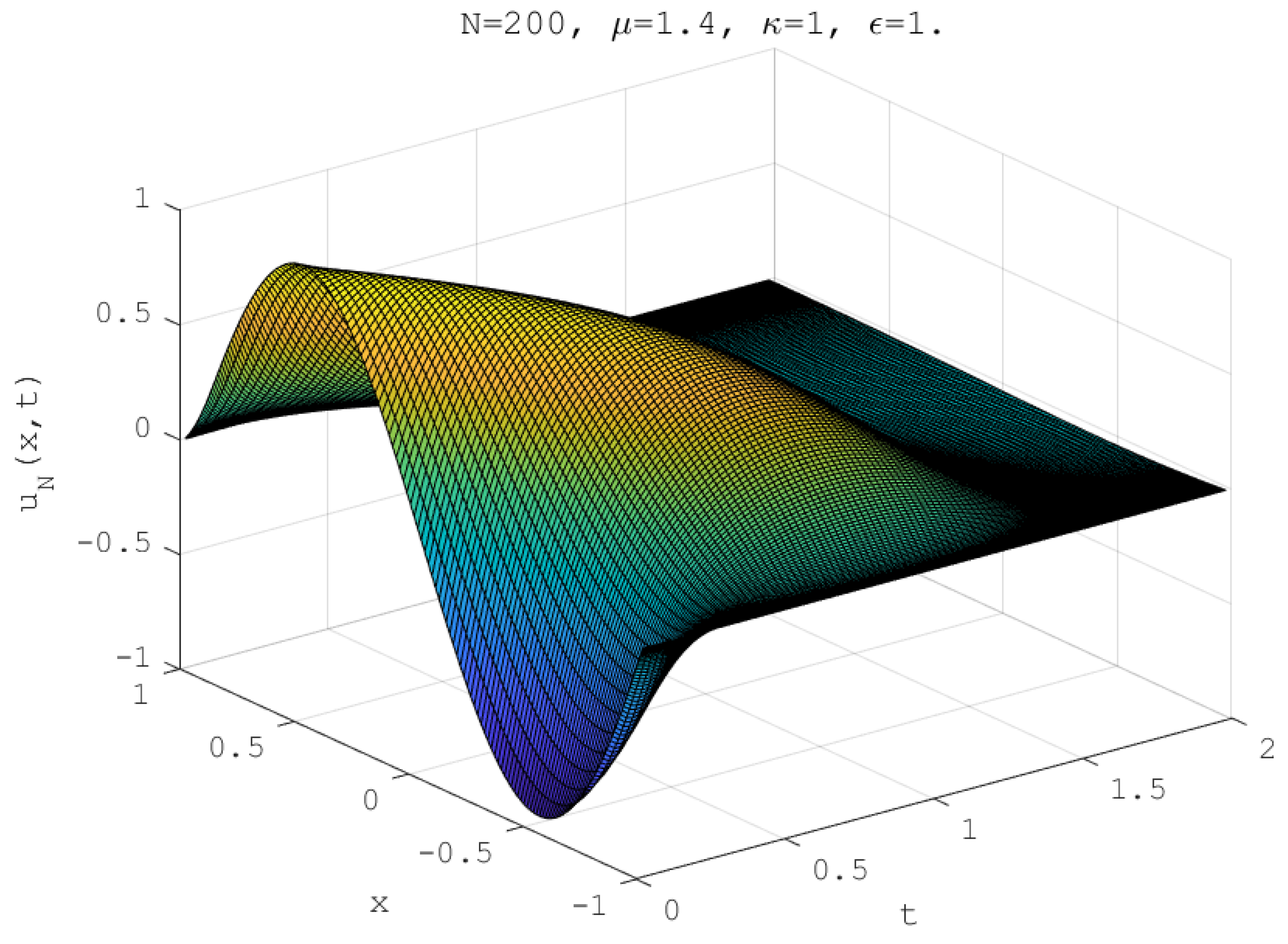
Figure 3.
Numerical solution for Example 3 of with .
Figure 3.
Numerical solution for Example 3 of with .
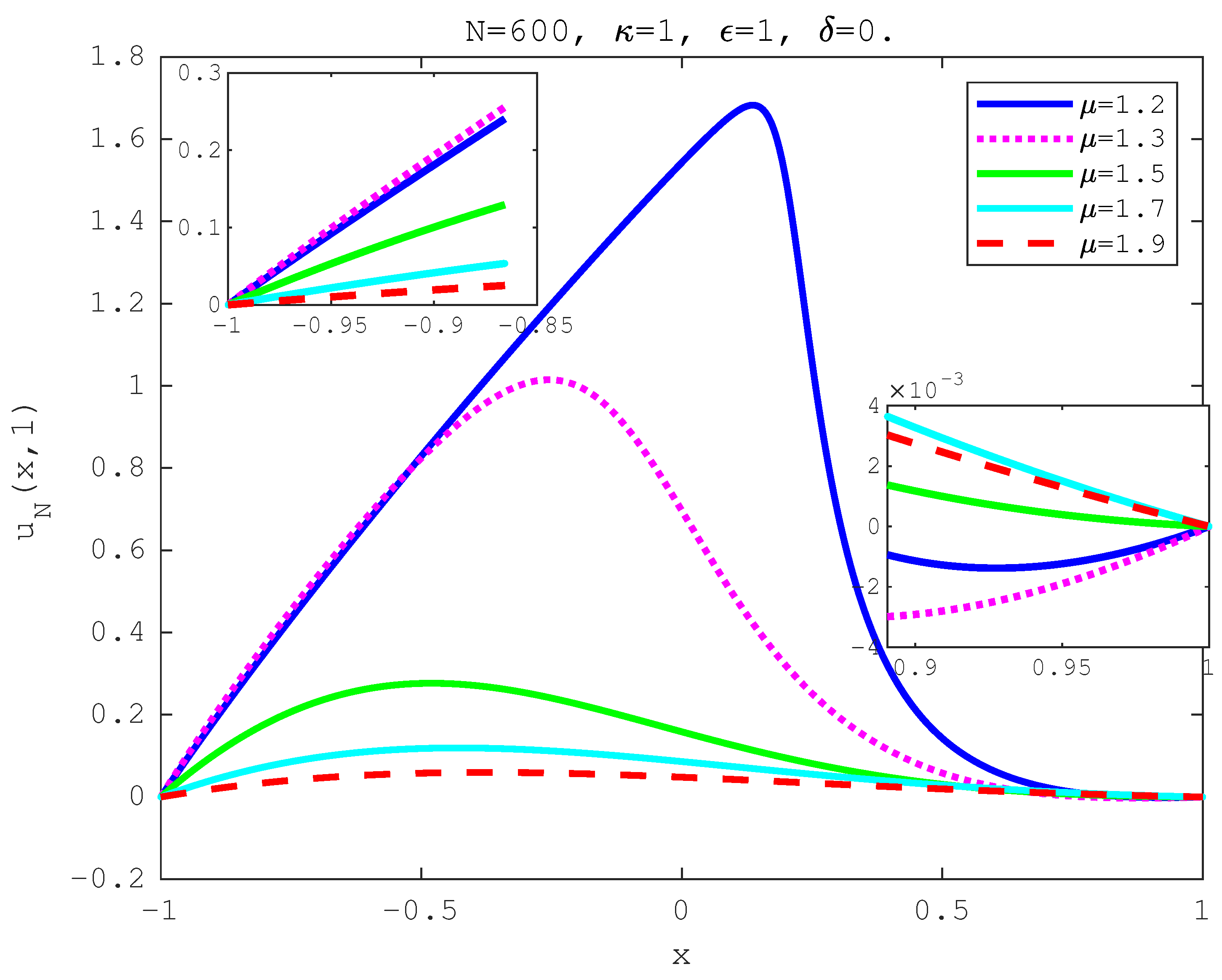
Figure 4.
Numerical solution for Example 3 of with .
Figure 4.
Numerical solution for Example 3 of with .
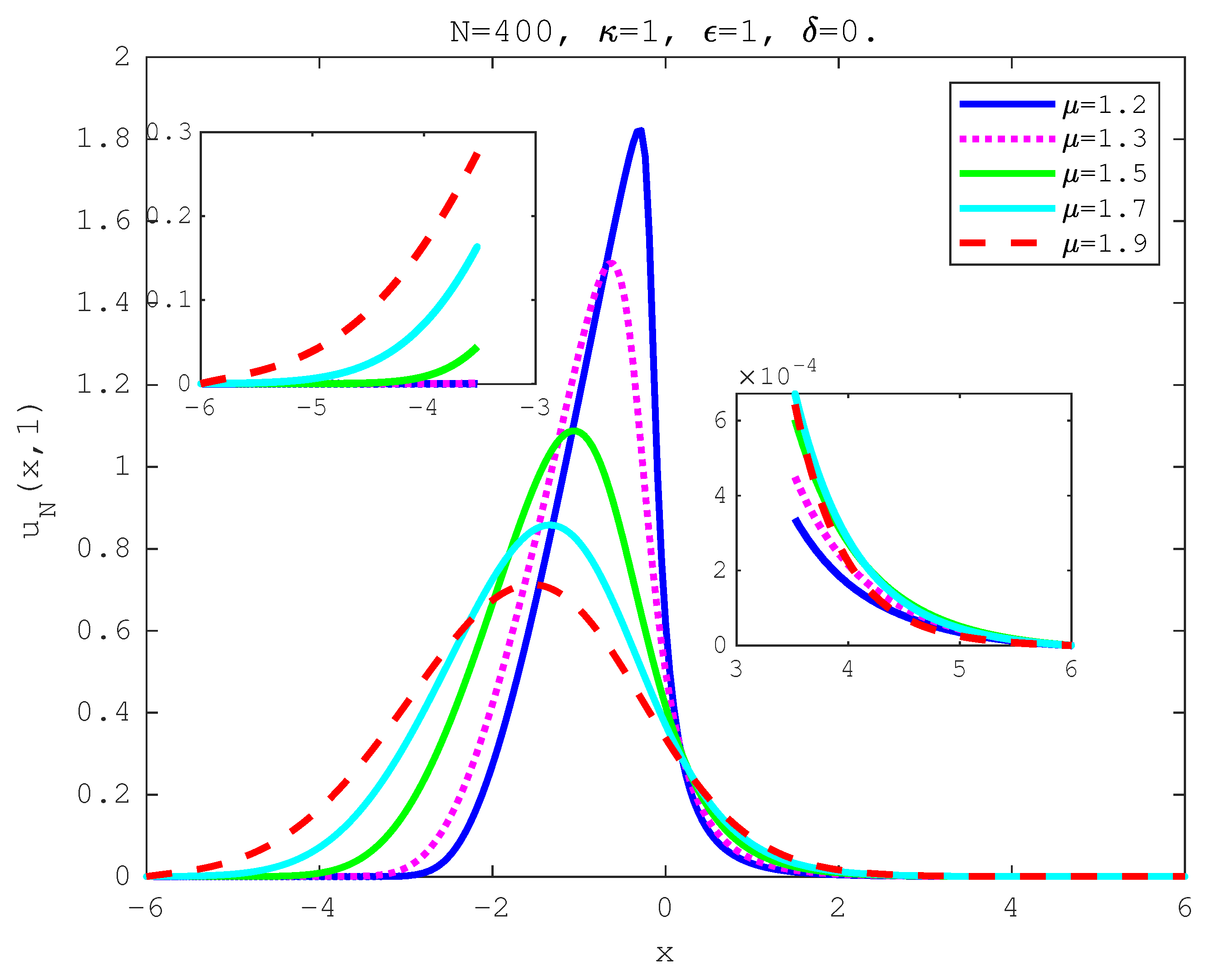
Figure 5.
Numerical solution for Example 3 of with .
Figure 5.
Numerical solution for Example 3 of with .
Figure 6.
Numerical solution for Example 3 of with .
Figure 6.
Numerical solution for Example 3 of with .
Figure 7.
Numerical solution for Example 3 of with .
Figure 7.
Numerical solution for Example 3 of with .
Figure 8.
Numerical solution for Example 3 of with .
Figure 8.
Numerical solution for Example 3 of with .
Figure 9.
Numerical solution for Example 3 of with .
Figure 9.
Numerical solution for Example 3 of with .
Table 1.
The numerical errors of Example 1 with C2 solution ().
Table 1.
The numerical errors of Example 1 with C2 solution ().
| [33] | | [33] | | [33] | |
|---|
| 10 | 5.811 × 10 | 1.0898 × 10 | 2.441 × 10 | 8.4114 × 10 | 7.771 × 10 | 1.3961 × 10 |
| 20 | 2.001 × 10 | 5.1711 × 10 | 6.381 × 10 | 2.8558 × 10 | 1.441 × 10 | 3.3180 × 10 |
| 40 | 6.501 × 10 | 3.8736 × 10 | 2.821 × 10 | 7.4061 × 10 | 6.001 × 10 | 7.5808 × 10 |
| 80 | 8.351 × 10 | 1.2290 × 10 | 3.841 × 10 | 3.6507 × 10 | 1.521 × 10 | 1.1427 × 10 |
| 160 | 4.721 × 10 | 1.8164 × 10 | 2.231 × 10 | 1.5149 × 10 | 1.541 × 10 | 1.7109 × 10 |
Table 2.
Errors of Example 2 with solution C1 ().
Table 2.
Errors of Example 2 with solution C1 ().
| N | | | | | | |
|---|
| 4 | 1.781 × 10 | 1.191 × 10 | 9.844 × 10 | 1.091 × 10 | 9.028 × 10 | 4.519 × 10 |
| 8 | 5.110 × 10 | 3.488 × 10 | 2.818 × 10 | 2.931 × 10 | 2.610 × 10 | 4.833 × 10 |
| 12 | 2.173 × 10 | 1.373 × 10 | 1.016 × 10 | 1.448 × 10 | 1.699 × 10 | 3.235 × 10 |
| 16 | 2.618 × 10 | 1.550 × 10 | 1.160 × 10 | 1.732 × 10 | 2.501 × 10 | 5.182 × 10 |
| 20 | 1.200 × 10 | 1.299 × 10 | 1.241 × 10 | 1.474 × 10 | 1.302 × 10 | 1.258 × 10 |
Table 3.
Errors of Example 2 with solution C1 ().
Table 3.
Errors of Example 2 with solution C1 ().
| N | | | | | |
|---|
| 4 | 2.282 × 10 | 2.901 × 10 | 1.322 × 10 | 2.338 × 10 | 1.605 × 10 |
| 8 | 9.931 × 10 | 5.828 × 10 | 2.701 × 10 | 3.397 × 10 | 1.821 × 10 |
| 12 | 3.315 × 10 | 2.504 × 10 | 1.210 × 10 | 1.889 × 10 | 1.075 × 10 |
| 16 | 3.008 × 10 | 2.379 × 10 | 1.493 × 10 | 2.353 × 10 | 1.419 × 10 |
| 20 | 1.174 × 10 | 2.498 × 10 | 1.443 × 10 | 1.282 × 10 | 2.776 × 10 |
Table 4.
Errors of Example 2 with solution C1 ().
Table 4.
Errors of Example 2 with solution C1 ().
| N | | | | | | |
|---|
| 4 | 2.131 × 10 | 1.509 × 10 | 1.068 × 10 | 5.353 × 10 | 1.900 × 10 | 9.521 × 10 |
| 8 | 3.355 × 10 | 3.035 × 10 | 2.745 × 10 | 2.247 × 10 | 1.663 × 10 | 1.361 × 10 |
| 12 | 3.806 × 10 | 3.632 × 10 | 3.467 × 10 | 3.158 × 10 | 2.745 × 10 | 2.500 × 10 |
| 16 | 9.076 × 10 | 8.868 × 10 | 8.618 × 10 | 8.188 × 10 | 7.522 × 10 | 7.119 × 10 |
| 20 | 2.220 × 10 | 1.110 × 10 | 1.110 × 10 | 5.551 × 10 | 2.082 × 10 | 2.776 × 10 |
Table 5.
Errors and of Example 2 with solution C2 ().
Table 5.
Errors and of Example 2 with solution C2 ().
| | | | | | | | | |
|---|
| | Ord | | Ord | | Ord | | Ord |
|---|
| 8 | 3.744 × 10 | - | 4.300 × 10 | - | 4.544 × 10 | - | 2.319 × 10 | - |
| 16 | 6.835 × 10 | 2.45 | 8.416 × 10 | 2.35 | 1.331 × 10 | 1.77 | 1.350 × 10 | 0.78 |
| 32 | 1.072 × 10 | 2.67 | 1.877 × 10 | 2.16 | 3.968 × 10 | 1.75 | 7.138 × 10 | 0.92 |
| 64 | 1.607 × 10 | 2.74 | 4.121 × 10 | 2.19 | 1.150 × 10 | 1.79 | 3.632 × 10 | 0.97 |
| 128 | 2.482 × 10 | 2.69 | 8.961 × 10 | 2.20 | 3.327 × 10 | 1.79 | 1.829 × 10 | 0.99 |
| 256 | 3.946 × 10 | 2.65 | 1.950 × 10 | 2.20 | 9.585 × 10 | 1.80 | 9.166 × 10 | 1.00 |
| 512 | 6.369 × 10 | 2.63 | 4.245 × 10 | 2.20 | 2.757 × 10 | 1.80 | 4.588 × 10 | 1.00 |
Table 6.
Errors and of Example 2 with solution C2 ().
Table 6.
Errors and of Example 2 with solution C2 ().
| | | | | | | | | |
|---|
| | Ord | | Ord | | Ord | | Ord |
| 8 | 4.526 × 10 | - | 1.453 × 10 | - | 9.694 × 10 | - | 5.743 × 10 | - |
| 16 | 5.361 × 10 | 6.40 | 1.066 × 10 | 7.09 | 5.753 × 10 | 7.40 | 3.732 × 10 | 7.27 |
| 32 | 1.061 × 10 | 5.66 | 7.197 × 10 | 7.21 | 3.757 × 10 | 7.26 | 2.171 × 10 | 7.43 |
| 64 | 1.072 × 10 | 6.63 | 4.430 × 10 | 7.34 | 2.126 × 10 | 7.47 | 1.183 × 10 | 7.52 |
| 128 | 7.944 × 10 | 10.40 | 6.140 × 10 | 6.17 | 5.207 × 10 | 5.35 | 4.952 × 10 | 4.58 |
Table 7.
Errors and of Example 2 with solution C2 ().
Table 7.
Errors and of Example 2 with solution C2 ().
| | | | | | | | | |
|---|
| | Ord | | Ord | | Ord | | Ord |
| 8 | 8.700 × 10 | - | 2.008 × 10 | - | 2.608 × 10 | - | 2.659 × 10 | - |
| 16 | 2.745 × 10 | 1.66 | 3.490 × 10 | 2.52 | 2.875 × 10 | 3.18 | 1.369 × 10 | 4.28 |
| 32 | 9.543 × 10 | 1.52 | 6.934 × 10 | 2.33 | 3.740 × 10 | 2.94 | 8.736 × 10 | 3.97 |
| 64 | 3.160 × 10 | 1.59 | 1.317 × 10 | 2.40 | 4.672 × 10 | 3.00 | 5.404 × 10 | 4.01 |
| 128 | 1.049 × 10 | 1.59 | 2.509 × 10 | 2.39 | 5.866 × 10 | 2.99 | 3.380 × 10 | 4.00 |
| 256 | 3.468 × 10 | 1.60 | 4.768 × 10 | 2.40 | 7.357 × 10 | 3.00 | 2.120 × 10 | 3.99 |
| 512 | 1.145 × 10 | 1.60 | 9.050 × 10 | 2.40 | 9.206 × 10 | 3.00 | 1.476 × 10 | 3.84 |
Table 8.
Errors and of Example 2 with solution C2 ().
Table 8.
Errors and of Example 2 with solution C2 ().
| | | | | | | | | |
|---|
| | Ord | | Ord | | Ord | | Ord |
| 8 | 1.163 × 10 | - | 1.331 × 10 | - | 1.202 × 10 | - | 1.302 × 10 | - |
| 16 | 1.165 × 10 | 6.64 | 9.526 × 10 | 7.13 | 6.495 × 10 | 7.53 | 7.022 × 10 | 7.53 |
| 32 | 1.180 × 10 | 6.63 | 6.321 × 10 | 7.24 | 3.020 × 10 | 7.75 | 4.644 × 10 | 7.24 |
| 64 | 1.122 × 10 | 6.72 | 3.846 × 10 | 7.36 | 1.316 × 10 | 7.84 | 1.643 × 10 | 4.82 |
| 128 | 1.047 × 10 | 6.74 | 5.762 × 10 | 6.06 | 5.529 × 10 | 4.57 | 1.715 × 10 | 6.58 |


