A Comparison Study of Time-Domain Computation Methods for Piecewise Smooth Fractional-Order Circuit Systems

Abstract

The role of fractional calculus in circuit systems has received increased attention in recent years. In order to evaluate the effectiveness of time-domain calculation methods in the analysis of fractional-order piecewise smooth circuit systems, an experimental prototype is developed, and the effects of three typical calculation methods in different test scenarios are compared and studied in this paper. It is proved that Oustaloup’s rational approximation method usually overestimates the peak-to-peak current and brings in the pulse–voltage phenomenon in piecewise smooth test scenarios, while the results of the two iterative recurrence-form numerical methods are in good agreement with the experimental results. The study results are dedicated to provide a reference for efficiently deploying calculation methods in fractional-order piecewise smooth circuit systems. Some quantitative analysis results are concluded in this paper.

1. Introduction

In recent decades, the concepts of fractional calculus and the related techniques have been gaining momentum in circuit system fields [1,2,3]. It has been confirmed that exploring the potential fractional-order characteristics of electronic components is helpful for both the condition monitoring of components and the reliability design of circuit systems [4,5,6,7,8]. An increasing body of evidence suggests that the fractional-order characteristic is widely distributed in electronic components [9,10,11], such as ultracapacitors (UCs), lithium batteries, and non-solid electrolytic capacitors. Moreover, introducing fractional-order elements (or constant phase elements—CPEs) to traditional circuit and control systems can enhance the design flexibility [12,13,14].

In order to better describe the characteristics of circuit systems with fractional-order components, it is of necessity to develop a set of reliable calculation and analysis methods. Basically, the lumped parameter model with fractional-order differential equations is a well-established approach to quantify the characteristics of fractional-order circuit systems, and a number of calculation and analysis works have been proposed for such systems—definition-based methods [15], rational approximation methods [16,17,18], and numerical methods [19,20,21], to name but a few. The methods listed above have been applied to the modeling and analysis of a wide variety of fractional-order circuit systems [22,23,24].

To the best of the authors’ knowledge, most existing calculation and analysis methods are applied only to continuous fractional-order circuit systems, for instance, the discussion on the convergence issue of solutions for continuous cobweb models in Ref. [25] and the study on the existence and uniqueness of the solution of Hadamard fractional Itô–Doob stochastic integral equations in Ref. [26]. However, existing works are rarely applied to piecewise smooth ones [27,28,29]. In practice, the piecewise-smooth characteristic is common in circuit systems, especially for those with semiconductor switching devices, and such a characteristic may bring in effects on the accuracy of numerical methods. Therefore, it is worthwhile to compare and evaluate the effectiveness of existing methods in analyzing piecewise smooth fractional-order systems.

In allusion to the state of the art, this work tries to unfold the applicability of three typical calculation methods for piecewise smooth fractional-order circuit systems. The rest of the work is organized as follows: test scenarios are established in Section 1, in which a non-solid aluminum electrolytic capacitor is employed in the test bench since this kind of component has been confirmed to have frequency-related fractional-order characteristics in a wide frequency band [11]. Section 2 deduces the solutions of the test scenarios by different approaches. Section 3 compares and discusses the results of different approaches, while Section 4 concludes the work.

2. Test Bench Settings and Mathematical Model

2.1. Test Bench Settings

In a previous work, it was confirmed that the electrode surface in the capacitor has an infinite self-similar structure, and the particle distribution law in it has a long-tail effect under the electric field, which is suitable to be described by the fractional equivalent impedance model [11]. The internal structure and fractional-order equivalent impedance circuit is presented in Figure 1.

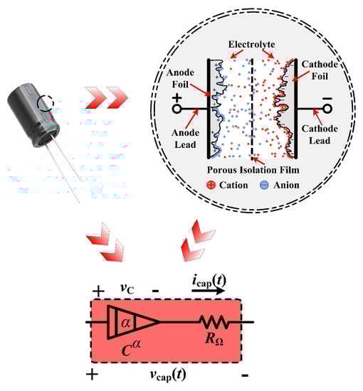
Figure 1. Internal structure and fractional-order equivalent impedance circuit model of non-solid aluminum electrolytic capacitors.

In the above figure, the symbol C is the nominal capacitance of the capacitor, while the symbol $\alpha$ is an estimated fractional order of 0 to 1, and the symbol $R_{\Omega }$ is the equivalent series resistance of the capacitor. A test bench is established in this section, which contains such a capacitor. The schematic of this test bench is displayed in Figure 2.

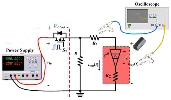
Figure 2. Schematic of the test bench.

The design of the test bench refers to the previous work [30], in which a type GPS-3303C 3-channel isolated dc power supply is adopted to provide power, and an oscilloscope is employed to record the data. In the platform, a type STP80NF70 power MOSFET $S_T$ is adopted, the gate-source voltage of which is controlled by a driving circuit. As a result, the test bench will work in charging and discharging the cycle working mode, so the circuit can be deemed as a piecewise smooth circuit system. On the right side of the red dash line in Figure 2, the resistor $R_1=5\Omega$ provides a discharging path for the capacitor, while $R_2=10\Omega$ is mainly used as the current sensing and limiting resistor. The circuit in the box with a red background is the fractional-order equivalent circuit of a $10\mathsf{\mu }\mathrm{F}$ Rubycon PX series non-solid aluminum electrolytic capacitor. The voltage and the current of the capacitor are $v_{cap}\left(t\right)$ and $i_{cap}\left(t\right)$, respectively, and two probes of the oscillascope are used to observe them. In addition, the voltage of the equivalent CPE is assumed to be $v_c\left(t\right)$. A glimpse of the experimental scene is given in Figure 3.

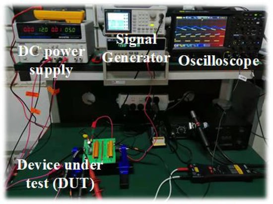
Figure 3. A glimpse of the experimental scene.

2.2. Mathematical Model

The test platform can be regarded as a charge–discharge circuit for the non-solid aluminum electrolytic capacitor. One can find that there is only one energy-storage component in the platform, so the interferences and errors are minimized compared with the schemes with rational approximation methods or those with magnetic elements. In the following parts, the test platform will be operated in two test scenarios to verify the applicability of different calculation and analysis methods.

According to the fractional-order equivalent impedance circuit of the capacitor in Figure 1, the current $i_{cap}\left(t\right)$ and the voltage $v_{cap}\left(t\right)$ of the capacitor satisfy the following relationships:

$$\left\{\begin{array}{c}{i}_{cap}\left(t\right)=C·{\displaystyle \frac{d^{\alpha }{v}_c\left(t\right)}{d{t}^{\alpha }}}\hfill \\ v_{cap}\left(t\right)=v_c\left(t\right)+R_{\Omega }·C·{\displaystyle \frac{d^{\alpha }{v}_c\left(t\right)}{d{t}^{\alpha }}},\hfill \end{array}\right.$$

(1)

It is noteworthy that the nominal capacitance C is 10 $\mathsf{\mu }$F in this work, while $R_{\Omega }$ and the fractional-order $\alpha$ related to the fractional-order characteristics of the capacitor can be identified by using the method proposed in a previous work [11], wherein their values are $0.8852$, $1.2629\Omega$, respectively.

In order to validate different methods, we established two groups of test scenarios, the basic and the advanced. In the basic test group, we consider two operating modes. The first one is sinusoidal mode, where the power supply is a single phase AC power supply with a pre-determined frequency. The second one is step mode, where a DC power supply is employed as the source and the power MOSFET $S_T$ is turned on at time $t=0$ with a constant forward voltage drop $V_{ds\left(on\right)}=0.7$ V.

• The state of the sinusoidal mode can be governed by

  $$v_c\left(t\right)+(R_2+R_{\Omega })·C·{\displaystyle \frac{d^{\alpha }{v}_c\left(t\right)}{d{t}^{\alpha }}}=v_{in}\left(t\right)-V_{ds\left(on\right)},$$

  (2)

  where $v_{in}\left(t\right)=K·sin\left(\omega t\right)$ is a sinusoidal function. K is the predetermined magnitude of the signal, $\omega =2\pi f_s$ is the angular frequency, and $f_s$ is the frequency of the sinusoidal function.
• The state of the step mode can be governed by

  $$v_c\left(t\right)+(R_2+R_{\Omega })·C·{\displaystyle \frac{d^{\alpha }{v}_c\left(t\right)}{d{t}^{\alpha }}}=V_{in}-V_{ds\left(on\right)},$$

  (3)

  in which $V_{in}$ is a predetermined constant value.

In the first group of test scenarios, the test bench works under continuous mode or step response mode. This group are used to assess the feasibility of different calculation methods.

In the second group of the test scenario, the power MOSFET $S_T$ is controlled by a periodic square waveform with a duty ratio D = 0.5 and a variable frequency $f_s$ from 100 Hz to 1 kHz. The performance of the circuit under test in one steady-state cycle $T_s$ can be governed by

• Charge performance in $t\in [k{T}_s,k{T}_s+D{T}_s]$ is

  $$v_{cap}\left(t\right)=V_{in}-V_{ds\left(on\right)}-R_2·i_{cap}\left(t\right),$$

  (4)

  where k is the k-th switching cycle, $T_s$ is the switching period, and

  $$\begin{array}{cc}\hfill V_{in}-V_{ds\left(on\right)}& =v_{cap}\left(t\right)+R_2·i_{cap}\left(t\right)\hfill \\ \hfill & =v_c\left(t\right)+(R_2+R_{\Omega })·C·{\displaystyle \frac{d^{\alpha }{v}_c\left(t\right)}{d{t}^{\alpha }}}.\hfill \end{array}$$

  (5)
• Discharge performance in $t\in [k{T}_s+D{T}_s,(k+1)T_s]$ is

  $$v_{cap}\left(t\right)=-(R_1+R_2)·i_{cap}\left(t\right),$$

  (6)

  and

  $$\begin{array}{cc}\hfill 0& =v_{cap}\left(t\right)+(R_1+R_2)·i_{cap}\left(t\right)\hfill \\ \hfill & =v_c\left(t\right)+(R_1+R_2+R_{\Omega })·C·{\displaystyle \frac{d^{\alpha }{v}_c\left(t\right)}{d{t}^{\alpha }}}.\hfill \end{array}$$

  (7)

In the second group of test scenarios, the capacitor of the test bench will be charged and discharged cycle by cycle, and thus the circuit under test is a typical piecewise smooth circuit system.

One can find that, to reveal the time-domain performance of these two scenarios, the voltage $v_C$ should be calculated. However, this voltage is an equivalent quantity of the CPE, and thus one cannot probe it directly and has to solve the fractional-order differential Equations (2)–(7), which are all fractional-order differential equations with constant coefficients. Rewrite these equations to the following generalized form:

$$a_{1i}·{\displaystyle \frac{d^{\alpha }x}{d{t}^{\alpha }}}+a_{0i}·x=u_i,$$

(8)

where $i=1,2,3,4$, $x=v_C$ is the only state variable of the circuit, and the coefficients are: $a_{11}=a_{12}=a_{13}=(R_2+R_{\Omega })C$, $a_{14}=(R_1+R_2+R_{\Omega })C$, $a_{01}=a_{02}=a_{03}=a_{04}=1$, $u_1=K·sin\left(\omega t\right)-V_{ds\left(on\right)}$, $u_2=u_3=V_{in}-V_{ds\left(on\right)}$, and $u_4=0$.

All the coefficients are predetermined in their own time intervals. Meanwhile, the initial conditions of Equation (8) are continuous in their own domains of definition, and hence according to Theorem 3.2 of Ref. [31], fractional-order differential Equation (8) has unique solutions. At this time, the initial values problem of fractional-order differential equations arises.

3. Computation Approaches

In this section, the principles of some related techniques are introduced first. Then three different approaches are applied to calculate Equations (2)–(7), and the results are adopted for validation and comparison. The first calculation method is a numerical calculation method, that is, the fractional Adams–Bashforth–Moulton-type method (F-ABM) [21]. The second calculation method is based on the Gr$\ddot{u}$nwald–Letnikov (G-L) definition [15]. To obtain solutions by using the first and the second methods, the stroboscopic map technique should be applied [32]. The third calculation method is Oustaloup’s rational approximation method [16], which will be conducted by using the state-space averaging (SSA) technique [33].

3.1. Preliminaries: Principles of Some Related Techniques

3.1.1. Stroboscopic Map Technique

One can always apply the most calculation approaches to calculate fractional-order differential equations in continuous cases directly. However, in discontinuous cases, or the piecewise smooth case discussed in this work, one may have to face a different situation, for example, the sign function of $f\left(x\right)=sign\left(x\right)$, which has the value of 1 for all $x>0$ and the value of $-1$ for all $x<0$, and Figure 4.

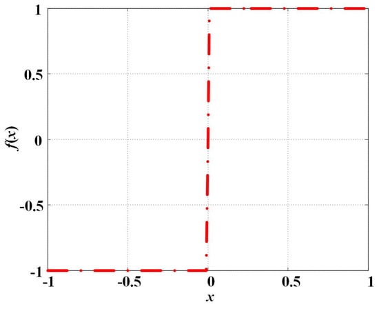
Figure 4. A graph of typical $sign\left(x\right)$ function.

The sign function of $f\left(x\right)=sign\left(x\right)$ appears in a variety of piecewise smooth fractional systems, which creates the initial value problem at the discontinuous point $x=0$, and one needs to physically interpret initial conditions at this point.

In the step mode of the basic test scenario, the proposed test bench also experiences a similar situation like the sign function. In addition, in the advanced test scenario, the capacitor experiences a recurrence of charging and discharging behaviors in each switching cycle, and thus the test bench will be in continuous state switching. Along with the on- and off operations of the power MOSFET $S_T$, there is a set of discontinuous points. Accordingly, a technique called stroboscopic map should be employed in both analytical and numerical calculations. This technique has widely been adopted in the dynamic analysis of piecewise-smooth systems and switching power converters. By this technique, the dynamic behavior of the test circuit at each switching state $S_n$ will be collected in one switching cycle, that is, the solution $x_n$ of the previous switching state at time $t_n$ will be employed as the initial value of the next switching state, and thus a cycle-by-cycle calculation can be carried out. The principle of the stroboscopic map technique is depicted in Figure 5.

Figure 5. Principle of stroboscopic map technique.

3.1.2. State-Space Averaging (SSA) Technique

In practice, some methods are difficult to be directly used in the advanced test scenario of this work. In allusion to this, the SSA technique can be exploited, by which the steady-state characteristic analysis can be achieved. By this technique, the average value of $v_c\left(t\right)$ in one switching cycle can be expressed by

$${⟨v_c⟩}_{T_s}={\displaystyle \frac{1}{T_s}}{\int }_{t_0}^{t_0+T_s}{v}_c\left(t\right)dt$$

(9)

Accordingly, in the steady state, when the low-frequency hypothesis and the small ripple hypothesis are satisfied, the test platform in the discontinuous case can be governed by the following SSA model:

$$\begin{array}{cc}\hfill & (R_2+R_{\Omega })·C·{\displaystyle \frac{d^{\alpha }{⟨v_c⟩}_{T_s}}{d{t}^{\alpha }}}+{⟨v_c⟩}_{T_s}\hfill \\ \hfill & +\left[1-d\left(t\right)\right]·R_1·C·{\displaystyle \frac{d^{\alpha }{⟨v_c⟩}_{T_s}}{d{t}^{\alpha }}}=d\left(t\right)\left[V_{in}-V_{ds\left(on\right)}\right],\hfill \end{array}$$

(10)

in which the terms ${⟨v_c⟩}_{T_s}$ and $d\left(t\right)$ can be decomposed into DC terms $V_c$ and D, AC terms ${\widehat{v}}_c$ and $\widehat{d}$, as follows:

$$\left\{\begin{array}{c}{⟨v_c⟩}_{T_s}=V_c+{\widehat{v}}_c\hfill \\ d\left(t\right)=D+\widehat{d}\hfill \end{array}\right.$$

(11)

3.2. Solutions of the Test Bench

3.2.1. Solutions Obtained by G-L Definition

According to the G-L definition, the fractional-order derivative of state variable $x\left(t\right)$ can be written in the following discrete form [15]:

$$\begin{array}{cc}\hfill {\displaystyle \frac{d^{\alpha }x\left(t\right)}{d{t}^{\alpha }}}& \approx {\displaystyle \frac{1}{h^{\alpha }}}\sum _{j=0}^{t/h}{p}_j^{\alpha }{x}_{t-jh}\hfill \\ \hfill & ={\displaystyle \frac{1}{h^{\alpha }}}\left[x_t+\sum _{j=1}^{t/h}{p}_j^{\alpha }{x}_{t-jh}\right],\hfill \end{array}$$

(12)

where h is the predetermined discrete step size, and $p_j^{\alpha }$ can be deduced by

$$p_0^{\alpha }=1,p_j^{\alpha }=\left(1-{\displaystyle \frac{1+\alpha }{j}}\right)p_{j-1}^{\alpha }.$$

(13)

Introducing Equation (13) into Equation (12) leads to the following recurrence form solution:

$$x_t={\displaystyle \frac{1}{a_{1i}+h^{\alpha }{a}_{0i}}}\left[h^{\alpha }{u}_{i,t}-\sum _{j=1}^{t/h}{p}_j^{\alpha }{x}_{t-jh}\right].$$

(14)

Then, one can obtain G-L based solutions of Equation (8) by point-by-point iteration of Equation (14). In addition, the numerical solutions of charging and discharging state in the advanced test scenario are collected in each switching cycle by the aforementioned stroboscopic map technique.

3.2.2. Solutions Obtained by F-ABM Method

In the case of $-1\le \alpha \le 1$, according to the definition of the F-ABM method [19], the initial value problem of the fractional-order system of Equation (8) can be determined by:

$$\begin{array}{cc}\hfill x(n+1)=x\left(0\right)& +{\displaystyle \frac{h^{\alpha }}{\Gamma (2+\alpha )}}f\left[t_{n+1},x^P(n+1)\right]\hfill \\ \hfill & +{\displaystyle \frac{h^{\alpha }}{\Gamma (2+\alpha )}}\sum _{j=0}^n{A}_{j,n+1}f\left[t_j,x\left(j\right)\right],\hfill \end{array}$$

(15)

where the term n is any integer, and $A_{j,n+1}$ is

$$A_{j,n+1}=\left\{\begin{array}{cc}\hfill & =n^{\alpha +1}-(n-\alpha ){(n+1)}^{\alpha },j=0\hfill \\ \hfill & ={(n-j+2)}^{\alpha +1}+{(n-j)}^{\alpha +1}\hfill \\ \hfill & -2{(n-j+1)}^{\alpha +1},1\le j\le n\hfill \\ \hfill & =1,j=n+1\hfill \end{array}\right.$$

(16)

The predictor $x^P(n+1)$ in Equation (15) is

$$x^P(n+1)=x_0+{\displaystyle \frac{1}{\Gamma \left(\alpha \right)}}\sum _{j=0}^n{B}_{j,n+1}f\left[t_j,x\left(j\right)\right],$$

(17)

in which the term $B_{j,n+1}$ is

$$B_{j,n+1}={\displaystyle \frac{h^{\alpha }}{\alpha }}\left[{(n+1-j)}^{\alpha }-{(n-j)}^{\alpha }\right].$$

(18)

Then the numerical solutions of Equation (8) can be obtained by Equation (15). Additionally, the numerical solutions of the charging and discharging state in the advanced test scenario will be collected in each switching cycle by the aforementioned stroboscopic map technique.

3.2.3. Solutions Obtained by Oustaloup’s Rational Approximation Method

By Oustaloup’s rational approximation method, a continuous filter can be designed in the frequency domain to achieve fractional-order calculus operations approximately. More specifically, by the Laplace transform, the fractional-order operation $\frac{d^{\alpha }}{d{t}^{\alpha }}$ can be transformed to an s-domain term $s^{\alpha }$, then the frequency domain characteristics of $s^{\alpha }$ can be approximated in the pre-defined frequency interval $[{\omega }_L,{\omega }_H]$ by an s-domain rational fraction function:

$${\displaystyle \frac{d^{\alpha }}{d{t}^{\alpha }}}\rightrightarrows K\prod _{i=-n}^n{\displaystyle \frac{s+z_i}{s+p_i}},$$

(19)

where the gain K, zeros $z_i$, and poles $p_i$ are

$$\left\{\begin{array}{c}K={(0.9·{\omega }_H)}^{\alpha }\hfill \\ z_i=-{\omega }_L·{\mu }^{\left(\right(i+N+0.5-0.5·\alpha )/(2·N+1\left)\right)}\hfill \\ p_i=-{\omega }_L·{\mu }^{\left(\right(k+N+0.5+0.5·\alpha )/(2·N+1\left)\right)},\hfill \end{array}\right.$$

(20)

respectively. The coefficient $\mu$ is

$$\mu ={\displaystyle \frac{{\omega }_H}{{\omega }_L}}.$$

(21)

Then the numerical solutions of Equation (8) can be obtained by encapsulating Equation (19) to a module in MATLAB/Simulink, such as those introduced in literature [16,17,18]. In addition, Equation (10) of the SSA technique should be applied. The block diagrams of the basic test scenario and the advanced test scenario are provided in Figure 6, where the block $s^{-\alpha }$ with red background is encapsulated according to Equation (19).

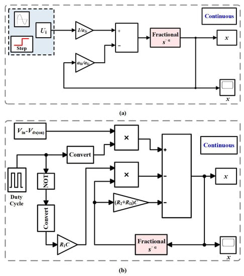
Figure 6. Principle block diagrams: (a) basic test scenario, (b) advanced test scenario.

4. Results Comparison and Evaluation

According to the scenario settings and the related derivation, comparative works are carried out in this section, and the numerical results are obtained by the F-ABM method, G-L definition, and Oustaloup’s method, collected in groups. In addition, experiment waveforms are provided as reference.

4.1. Results of Calculation and Simulation

The first group of results are from the basic test scenario. By using the aforementioned three approaches, one can obtain numerical simulation results as depicted in Figure 7. The second group of results is from the advanced test scenario, with the simulation results given in Figure 8. In both cases, the blue solid line represents the voltage of power supply, while the red dash-and-dot line corresponds to the results of Oustaloup’s rational approximation method, the black dash line corresponds to the results of G-L definition, and the green solid line corresponds to the results of the F-ABM method.

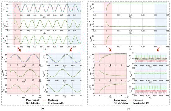
Figure 7. Comparison of basic test scenarios: (a) sinusoidal case, (b) step case.

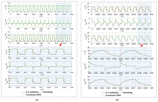
Figure 8. Comparison of advanced test scenarios: (a) advanced scenario with $f_s=100$ Hz, (b) advanced scenario with $f_s=200$ Hz.

In the above two figures, the sub-graphs with red and blue backgrounds refer to the enlarged parts.

In the sinusoidal case, it can be seen that the results of the three methods mesh well with each other in the steady state. There is a lag of around 0.5 ms between the voltage $v_c\left(t\right)$ and the voltage of the power supply, which is determined by the capacitance $C=10\mathsf{\mu }\mathrm{F}$ and the fractional order $\alpha =0.8852$ of the equivalent impedance model of the capacitor.

In step case, it can be seen that at the discontinuous point, the peak currents obtained by the three methods are almost the same, the value is around 1.0395 A. However, note that, the results obtained by three methods are slightly different at a steady state. In detail, the steady-state voltage calculated by Oustaloup’s method is about 0.1 V lower than the results obtained by the G-L definition and F-ABM method. In addition, the steady-state current calculated by Oustaloup’s method is about 0.01 A higher than the results obtained by the G-L definition and F-ABM method.

In advance test scenarios, it can be seen that the results of three methods mesh well with each other. However, note that there are spikes of the voltages $v_c\left(t\right)$ and $v_{cap}\left(t\right)$ at discontinuous points if one uses Oustaloup’s method. With the acceleration frequency $f_s$ of charge–discharge state transition, this spike phenomenon becomes obvious. In addition, the steady-state current $i_{cap}\left(t\right)$ and the voltage $v_{cap}\left(t\right)$ calculated by the three methods are slightly different. With the acceleration frequency $f_s$ of the charge–discharge state transition, this difference becomes obvious.

4.2. Evaluation and Discussion

In order to further validate the calculation results, experiment waveforms are provided in Figure 9 and Figure 10.

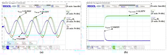
Figure 9. Experiment results of basic test scenarios: (a) sinusoidal case, (b) step case.

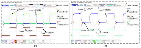
Figure 10. Experiment results of advanced test scenarios: (a) advanced scenario with $f_s=100$ Hz, (b) advanced scenario with $f_s=200$ Hz.

In Figure 9, the blue solid lines are the voltage $v_2\left(t\right)$ of the resistor $R_2$. It can be regarded as the sampling for the current $i_{cap}\left(t\right)$ flowing through the capacitor. The red solid lines correspond to the voltage of the power supply, the green solid line corresponds to the voltage $v_{cap}\left(t\right)$ of the capacitor.

It can be found that experimental waveforms are very similar to the theoretical calculation and simulation results. In order to assess the results of the calculation, statistical analysis was used to qualify different methods.

First of all, we compare the spike current $i_{spike}$, the averaged steady-state capacitor voltage ${\overline{v}}_{cap}$, and the averaged steady-state capacitor current ${\overline{i}}_{cap}$ in the step case in Table 1.

Table 1. Comparison of the spike current $i_{spike}$, the averaged steady-state capacitor voltage ${\overline{v}}_{cap}$, and the averaged steady-state capacitor current ${\overline{i}}_{cap}$ in step case.

	${\overline{\mathit{v}}}_{\mathit{cap}}$	${\overline{\mathit{i}}}_{\mathit{cap}}$	${\mathit{i}}_{\mathit{spike}}$
G-L definition	11.2894 V	≈1.29 mA	1.0012 A
F-ABM	11.3025 V	≈−0.2 mA	1.0308 A
Oustaloup’s	11.2816 V	0.0110 A	1.0379 A
Experiments	11.5570 V	≈1 mA	0.9869 A

From Table 1, it can be seen that most of the calculation results of the three methods have little deviation from the experimental results in the step case. However, compared with the other results, the averaged current ${\overline{i}}_{cap}$ obtained by Oustaloup’s method is too large. This current value is unreasonable because in both theory and practice, if the electric field applied to the capacitor is constant, the current of the capacitor should be in a trickle state.

Then, we compare the calculations results in sinusoidal case and advanced scenarios and list the peak-to-peak values obtained by different methods in Table 2.

Table 2. Comparison of peak-to-peak values of capacitor voltage $v_{cpp}$ and current $i_{cpp}$.

	In Sinusoidal Case	In Advanced Scenario with ${\mathit{f}}_{\mathit{s}}=100$ Hz	In Advanced Scenario with ${\mathit{f}}_{\mathit{s}}=200$ Hz
G-L definition	(0.5851 A, 21.9082 V)	(1.6848 A, 11.0712 V)	(1.6656 A, 10.6078 V)
F-ABM	(0.5908 A, 21.9414 V)	(1.6853 A, 10.7952 V)	(1.6686 A, 10.0280 V)
Oustaloup’s	(0.5514 A, 22.3235 V)	(1.9266 A, 11.6760 V)	(1.9088 A, 12.2848 V)
Experiments	(0.6211 A, 21.1210 V)	(1.6991 A, 11.6547 V)	(1.6624 A, 11.3748 V)

From Table 2, it can be seen that the calculation results of the three methods have little deviation from the experimental results in the sinusoidal case, which means that the three methods are applicable for continuous situations.

However, compared with other results, the peak-to-peak current $i_{pp}$ obtained by Oustaloup’s method is larger in advanced scenarios. In addition, one can observe pulse voltage signals at some edge time points in the simulation results obtained by Oustaloup’s method, which cannot be observed in both experiments and the results of the other two methods. In principle, this pulse voltage phenomenon mainly occurs at the on and off operation edges of the power MOSFET $S_T$. At these time points, the test circuit switches between charging and discharging states, just like the high-level and low-level signals of the sign function in Figure 6 undergo periodic switching. As a result, the state equation of the test circuit switches between Equation (5) and (7), and the test bench is a typical piecewise smooth circuit system.

Basically, the expressions of most frequency-domain rational approximation methods are the approximation of the amplitude–frequency or phase–frequency characteristics of ideal fractional calculus operators in a predetermined frequency band, and usually considering the situation of being continuously differentiable. However, at the boundary points of piecewise smooth scenarios, the state equation of the test bench is discontinuous and non-derivable. Therefore, the approximation results of the rational approximation method are not that effective. This pulse–voltage phenomena can also be explained by the Fourier transform of a step function.

5. Conclusions

This paper compares the effectiveness of the G-L definition based method, the F-ABM method, and Oustaloup’s rational approximation method for fractional-order piecewise smooth circuit systems. A test platform for verification is developed, in which a fractional-order component, a non-solid electrolytic capacitor, is adopted. The test platform can be operated under basic and advanced test scenarios. The basic scenario contains a continuous sinusoidal case and a step case, while the advanced scenario is the periodic charging and discharging operation of the capacitor.

Three computational methods work well in basic test scenarios, especially in the sinusoidal case, which indicates that these methods are effective in continuous situations. However, in the step case, the averaged current obtained by Oustaloup’s method is too large. In advance scenarios, the waveforms obtained by three methods are similar to the experimental results. Two iterative numerical calculation methods, G-L definition method and F-ABM method, perform well in $f_s=100$ Hz and $f_s=200$ Hz advanced scenarios, the deviation between their calculation results and the experimental results is small. However, applying Oustaloup’s method in advanced scenarios leads to large calculation deviations. Moreover, if one employs Oustaloup’s method in advanced scenarios, there is a pulse–voltage phenomenon when the circuit changes from the charging state to discharging state, which cannot be observed in both experiments and the results of the two iterative numerical calculation methods. The comparison and experimental verification results show that the G-L definition based method and F-ABM method are effective for fractional-order piecewise-smooth circuit systems.

The results provided by this research will provide more confidence for understanding the dynamics of real-world systems governed by fractional calculus. For those discrete- or continuous-time piecewise-smooth fractional-order dynamical systems, such as power electronic converters, which are typical piecewise smooth fractional-order circuit systems, if the fractional-order characteristics of passive components used in topology are considered, the discussion in the work provides a reference for effective deployment calculation methods.

References

- Elwakil, A. Fractional-Order Circuits and Systems: An Emerging Interdisciplinary Research Area. IEEE Circuits Syst. Mag. 2010, 10, 40–50. [Google Scholar] [CrossRef]
- Zhang, B.; Shu, X. Fractional-Order Electrical Circuit Theory (CPSS Power Electronics Series), 1st ed.; Springer: Singapore, 2022; pp. 39–54. [Google Scholar]
- Petráš, I. Fractional-Order Nonlinear Systems; Springer: Berlin/Heidelberg, Germany, 2011; pp. 43–54. [Google Scholar]
- Zou, C.; Zhang, L.; Hu, X.; Wang, Z.; Wik, T.; Pecht, M. A review of fractional-order techniques applied to lithium-ion batteries, lead-acid batteries, and supercapacitors. J. Power Sources 2018, 390, 286–296. [Google Scholar] [CrossRef]
- Zhang, L.; Kartci, A.; Elwakil, A.; Bagci, H.; Salama, K.N. Fractional-Order Inductor: Design, Simulation, and Implementation. IEEE Access 2021, 9, 73695–73702. [Google Scholar] [CrossRef]
- Allagui, A.; Elwakil, A.S.; Fouda, M.E. Revisiting the Time-Domain and Frequency-Domain Definitions of Capacitance. IEEE Trans. Electron Devices 2021, 68, 2912–2916. [Google Scholar] [CrossRef]
- Huang, Y.; Chen, X. A fractional-order equivalent model for characterizing the interelectrode capacitance of MOSFETs. IEEE COMPEL—Int. J. Comput. Math. Electr. Electron. Eng. 2022, 41, 1660–1676. [Google Scholar] [CrossRef]
- Chen, X.; Pei, M. Enhancing parameter identification of electrochemical double layer capacitors by fractional-order equivalent impedance models and Levy flight strategy. Int. J. Circuit Theory Appl. 2022. [Google Scholar] [CrossRef]
- Mondal, D.; Biswas, K. Packaging of Single-Component Fractional Order Element. IEEE Trans. Device Mater. Reliab. 2013, 13, 73–80. [Google Scholar] [CrossRef]
- Allagui, A.; Freeborn, T.J.; Elwakil, A.S.; Elwakil, A.S.; Fouda, M.E.; Maundy, B.J.; Radwan, A.G.; Said, Z.; Abdelkareem, M.A. Review of fractional-order electrical characterization of supercapacitors. J. Power Sources 2018, 400, 457–467. [Google Scholar] [CrossRef]
- Chen, X.; Xi, L.; Zhang, Y.; Ma, H.; Huang, Y.; Chen, Y. Fractional techniques to characterize non-solid aluminum electrolytic capacitors for power electronic applications. Nonlinear Dyn. 2019, 98, 3125–3141. [Google Scholar] [CrossRef]
- Freeborn, T.J. A Survey of Fractional-Order Circuit Models for Biology and Biomedicine. IEEE J. Emerg. Sel. Top. Circuits Syst. 2013, 3, 416–424. [Google Scholar] [CrossRef]
- Tripathy, M.C.; Mondal, D.; Biswas, K.; Sen, S. Experimental studies on realization of fractional inductors and fractional-order bandpass filters. Int. J. Circuit Theory Appl. 2015, 43, 1183–1196. [Google Scholar] [CrossRef]
- Jiang, Y.; Zhang, B.; Shu, X.; Wei, Z. Fractional-order autonomous circuits with order larger than one. J. Adv. Res. 2020, 25, 217–225. [Google Scholar] [CrossRef]
- Scherer, R.; Kalla, S.L.; Tang, Y.; Huang, J. The Grünwald–Letnikov method for fractional differential equations. Comput. Math. Appl. 2011, 62, 902–917. [Google Scholar] [CrossRef]
- Oustaloup, A.; Levron, F.; Mathieu, B.; Nanot, F.M. Frequency-band complex noninteger differentiator: Characterization and synthesis. IEEE Trans. Circuits Syst. I-Fundam. Theory Appl. 2000, 47, 25–39. [Google Scholar] [CrossRef]
- Malti, R.; Victor, S. CRONE Toolbox for system identification using fractional differentiation models. IFAC-Pap. OnLine 2015, 48, 769–774. [Google Scholar] [CrossRef]
- Xue, D.; Chen, Y. System Simulation Techniques with MATLAB® and Simulink®, 1st ed.; John Wiley & Sons: West Sussex, UK, 2013; pp. 85–90. [Google Scholar]
- Diethelm, K. The Analysis of Fractional Differential Equations: An Application-Oriented Exposition Using Differential Operators of Caputo Type; Springer: Berlin/Heidelberg, Germany, 2010; pp. 195–225. [Google Scholar]
- Momani, S.; Odibat, Z. Numerical approach to differential equations of fractional order. J. Comput. Appl. Math. 2007, 1, 96–110. [Google Scholar] [CrossRef]
- Owolabi, K.M.; Atangana, A. Numerical Methods for Fractional Differentiation; Springer Nature: Singapore, 2019; pp. 203–208. [Google Scholar]
- Chen, X.; Chen, Y. A Modeling and Analysis Method for Fractional-order DC-DC Converters. IEEE Trans. Power Electron. 2017, 32, 7034–7044. [Google Scholar] [CrossRef]
- Wei, Z.; Zhang, B.; Jiang, Y. Analysis and Modeling of Fractional-Order Buck Converter Based on Riemann-Liouville Derivative. IEEE Access 2019, 7, 162768–162777. [Google Scholar] [CrossRef]
- Li, G.; Lehman, B. Averaging Theory for Fractional Differential Equations. Fract. Calc. Appl. Anal. 2021, 24, 621–640. [Google Scholar] [CrossRef]
- Nagy, A.M.; Assidi, S.; Makhlouf, A.B. Convergence of solutions for perturbed and unperturbed cobweb models with generalized Caputo derivative. Bound. Value Probl. 2022, 89, 1–13. [Google Scholar] [CrossRef]
- Kahouli, O.; Makhlouf, A.B.; Mchiri, L.; Mchiri, L.; Rguigui, H. Hyers—Ulam stability for a class of Hadamard fractional Itô—Doob stochastic integral equations. Chaos. Soliton. Fract. 2021, 103, 2855–2866. [Google Scholar] [CrossRef]
- Danca, M.F. Synchronization of piecewise continuous systems of fractional order. Nonlinear Dyn. 2014, 78, 2065–2084. [Google Scholar] [CrossRef]
- Liu, X.; Hong, L.; Tang, D.; Yang, L. Crises in a fractional-order piecewise system. Nonlinear Dyn. 2021, 103, 2855–2866. [Google Scholar] [CrossRef]
- Alazman, I.; Alkahtani, B.S.T. Investigation of Novel Piecewise Fractional Mathematical Model for COVID-19. Fractal Fract. 2022, 6, 661. [Google Scholar] [CrossRef]
- Yang, Z.; Xi, L.; Zhang, Y.; Chen, X. An Online Parameter Identification Method for Non-solid Aluminum Electrolytic Capacitors. IEEE Trans. Circuits Syst. II Express Briefs 2022, 69, 3475–3479. [Google Scholar] [CrossRef]
- Podlubny, I. Fractional Differential Equations: An Introduction to Fractional Derivatives, Fractional Differential Equations, to Methods of Their Solution and Some of Their Applications; Academic Press: London, UK, 1998; pp. 124–125. [Google Scholar]
- Tse, C.K.; Xi, L.; Bernardo, M.D. Complex Behavior in Switching Power Converters. Proc. IEEE 2002, 90, 768–781. [Google Scholar] [CrossRef]
- Erickson, R.W.; Maksimovic, D. Fundamentals of Power Electronics, 2nd ed.; Kluwer Academic Publishers: Norwell, MA, USA, 2001; pp. 213–246. [Google Scholar]
Disclaimer/Publisher’s Note: The statements, opinions and data contained in all publications are solely those of the individual author(s) and contributor(s) and not of MDPI and/or the editor(s). MDPI and/or the editor(s) disclaim responsibility for any injury to people or property resulting from any ideas, methods, instructions or products referred to in the content. |
© 2023 by the authors. Licensee MDPI, Basel, Switzerland. This article is an open access article distributed under the terms and conditions of the Creative Commons Attribution (CC BY) license (https://creativecommons.org/licenses/by/4.0/).