Abstract
In the literature, different approaches that are employed in designing automatic voltage regulators (AVRs) usually model the AVR as a single-input-single-output system, where the input is the generator reference voltage, and the output is the generator voltage. Alternately, it could be thought of as a double-input, single-output system, with the excitation voltage change serving as the additional input. In this paper, unlike in the existing literature, we designed the AVR system as a sextuple-input single-output (6ISO) system. The inputs in the model include the generator reference voltage, regulator signal change, exciter signal change, amplifier signal change, generator output signal change, and the sensor signal change. We also compared the generator voltage responses for various structural configurations and regulator parameter choices reported in the literature. The effectiveness of numerous controllers is investigated; the proportional, integral and differential (PID) controller, the PID with second-order derivative (PIDD2) controller, and the fractional order PID (FOPID) controller are the most prevalent types of controllers. The findings reveal that the regulator signal change and the generator output signal change significantly impact the generator voltage. Based on these findings, we propose a new approach to design the regulator parameter to enhance the response to generator reference voltage changes. This approach takes into consideration changes in the generator reference voltage as well as the regulator signal. We calculate the regulator settings using a cutting-edge hybrid technique called the Particle Swarm Optimization African Vultures Optimization algorithm (PSO–AVOA). The effectiveness of the regulator design technique and the proposed optimization algorithm are demonstrated.
1. Introduction
Frequency and voltage are the two leading indicators of the quality of the electrical supply. Voltage is a local property, whereas frequency has a global aspect. Turbine regulators are used in electric power systems to control frequency, whereas synchronous machine excitation systems are used to control voltage. For example, a synchronous machine serves as the primary frequency and voltage controller [1]. In this regard, voltage regulation is discussed. A synchronous machine and a variety of compensating systems, including static compensating devices, can be used in practice to regulate voltage [2]. For a synchronous machine, controlling the excitation entails controlling the excitation voltage and current, which control the flux value of the machine [1]. The excitation regulator, mostly implemented in processor technology in today’s excitation systems, is the key component of the voltage regulation loops of synchronous machines. Their suitability for adopting different management regulations, altering the operation logic, being easily controllable, and monitoring various factors is a result of this [3]. The selection of the type and optimization of the regulator parameters have received the majority of the researchers’ attention in the related scientific literature to date. The standard proportional, integral, and differential (PID) controller is the most popular type of controller, which may be inferred from the literature [4,5]. The proportional term refers to using the all-pass gain factor to provide an overall control action proportional to the error signal. The integral term refers to minimizing steady-state errors through an integrator’s low-frequency compensation. The derivative term refers to improving transient response through a differentiator’s high-frequency compensation. As noted in [5], PID with a second-order derivative (PIDD2) controllers and fractional-order PID (FOPID) controllers [6,7,8,9] provide a further improvement in the system performance. Table 1 lists the main types of fundamental regulators found in AVR structures.

Table 1.
Types of regulators.
In the literature, the application of metaheuristic algorithms is considered essential for the optimization of controller settings. The goal function, known as the objective function or the fitness function, must be defined before an algorithm can be used to estimate the regulator parameters. A function’s mathematical definition includes the primary system variables and procedures necessary to appropriately specify the system responses. Table 2 lists the primary objective functions that estimate the AVR regulator parameters. Additionally, Figure 1 provides a list of numerous employed objective functions for estimating the parameters of an AVR regulator.
Table 2.
Objective functions commonly used in optimal controller design.
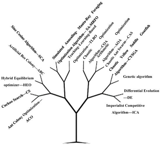
Figure 1.
The widely used metaheuristic algorithms used in estimating AVR parameters.
It is critical to emphasize these observations in light of the literature:
- It was observed how the generator voltage responded to the generator voltage’s reference value, which ranged from zero to one, while a step disturbance was present. In papers [3,4,5,6,7,8,9,10,11,12,13,14,15,16,17,18,19,20,21,22,23,24], this change in the reference value is illustrated.
- The impact of excitation voltage saturation was taken into consideration in numerous research works [22,25].
- Only one study [25] evaluated the value of the regulator parameters under network operation and within permitted voltage limits, when the generator voltage reference value was changed.
- The voltage response was shown in [3,4,5,6,7,8,9,10,11,12,13,14,15,16,17,18,19,20,21,22,23,24] when the reference value changed from zero to the nominal value for a fully loaded generator, which is undesirable in real-world applications.
Apart from the generator voltage reference value and the generator voltage itself, the excitation control system receives a variety of input signals in practice [22,25]. This includes limiters for the excitation current, the power system stabilizer signal, and others. Numerous limiters and control blocks handle excitation current management in today’s excitation regulation systems. Specifically, the generator’s current, as well as signals from the PSS, the voltage–frequency (VHz) limiter, and the fast limiters of the excitation current, are provided as input to the excitation regulation along with the signal of the generator’s real value of voltage. Excitation current and generator current are, therefore, both inputs. Any noise can, therefore, impact the excitation regulation mechanism on one of those signals.
On the other hand, many signals are restricted, and the regulator is designed to be wind-up resistant (anti-wind-up) [22]. A lot of details regarding modern AVR designs can be found in [25]. A control signal is created in the regulator by considering all of these signals. The regulator sends a control signal to the amplifier, which then uses it to control the thyristors in the rectifying bridge further. Potentially, disturbance signals that interfere with the original signal could be generated at each transmission location in the excitation regulation system. The results presented in [25] illustrated the impact of excitation voltage signal disturbance when evaluating the settings of the AVR control regulator. Bearing these considerations in mind, the purpose of this work’s research is apparent. The goal is to consider all possible impacts of disturbances in the system and then estimate the regulator’s parameters in light of these effects and changes to the generator voltage’s reference value. In order to achieve this, it is crucial to examine the impact of interference with the solutions suggested in the literature for the regulator’s parameters and design. A new mathematical formulation of the regulator should be put forward in order to accurately estimate the regulator parameters.
In this regard, this article investigates a system with six input quantities—five disturbance signals and one input reference signal—because there are five probable sources of disturbance signals.
The main contributions of the work are briefed as follows:
- We provided an innovative 6ISO AVR contour model for the first time in the literature based on the author’s knowledge.
- We explained the physical sense of the derived contour and tested the impact of all signals on the generator voltage waveforms.
- We derived the mathematical expressions for all signals in the derived contour.
- We proposed a novel strategy for identifying the parameters of the regulator.
- We compared the obtained results with the corresponding results presented in the literature.
The work is divided into numerous chapters for better understanding. A new 6ISO model of the AVR formulation is suggested in the second chapter, and the mathematical equations of the input–output interdependence are also provided. The third chapter suggests an innovative approach for estimating the AVR parameters. A comparison of the generator voltage response results for various systems from the literature is examined in the fourth chapter. In the fifth chapter, the results of finding the regulator parameters for the suggested approach and comparing the results with those of other methods are presented. The conclusion chapter provides a summary of the findings as well as suggestions for additional research.
2. Proposed 6ISO AVR Model
A synchronous machine, an amplifier, an exciter, a controller, and a sensor form the excitation control system. The synchronous machine is the main source of energy for electric energy systems (EES). The excitation of the synchronous machines is powered by a rectifier bridge (also referred to as an exciter). The regulator determines the control signals, while an amplifier device regulates the control angles. A sensor is used to measure the generating voltage. Figure 2 illustrates the block diagram of the AVR structure together with all the potential disturbances. The character “a” stands for the signal for a disturbance in each element in this figure. Each element is linearized using a first-order transfer function, as presented in the research works that address the AVR model [3,4,5,6,7,8,9,10,11,12,13,14,15,16,17,18,19,20,21,22,23,24]. In this way of linearization, each part is very simple and does not have many physical nonlinearities. The mathematical expressions and descriptions of elements are given in [3,4,5,6,7,8,9,10,11,12,13,14,15,16,17,18,19,20,21,22,23,24,25]. Table 3 provides values of the overall gain and time constants for each element.
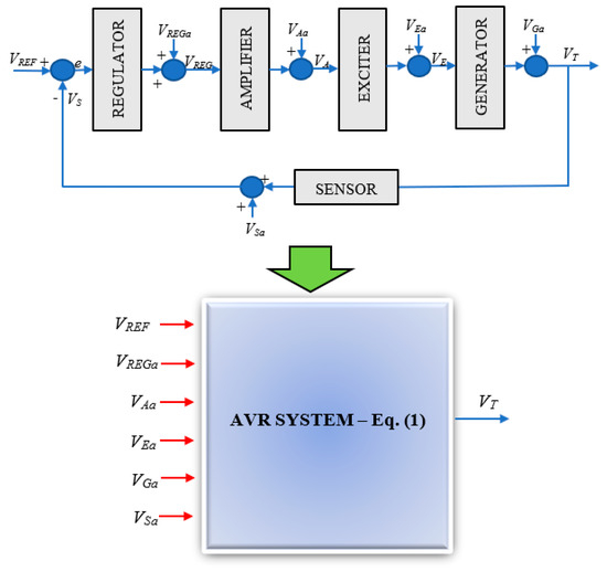
Figure 2.
The proposed 6ISO AVR model with six input signals.
Table 3.
Elements representation [3,4,5,6,7,8,9,10,11,12,13,14,15,16,17,18,19,20,21,22,23,24,25].
In the AVR structure shown in Figure 2, the relation between the generator voltage and the excitation voltage is expressed as follows:
while the corresponding expressions for the excitation voltage, exciter voltage, and regulator signal are expressed as follows:
where VREF represents the generator reference voltage, W represents the transfer function of each element in the presented block scheme, so that , and REG is a regulator of any type.
The previously given equations represent the set of equations of the 6ISO-AVR model. It is obvious that all equations are reduced to the expression given in [3,4,5,6,7,8,9,10,11,12,13,14,15,16,17,18,19,20,21,22,23,24] in cases where the noise/disturbance signals are zero.
3. Comparison of the Output Voltage Response and Literature Review
This chapter highlights the modeling results of how the generator and excitation voltage respond to different changes in the generator voltage, the excitation voltage, the output from the amplifier, the regulator, and the sensor. The findings shown are for two disturbances that are 0.05 pu and 0.07 pu. In these investigations, different regulator structures were taken into account, as well as the different regulator parameters obtained by numerous methods presented in the literature, as given in Table 4. The types of regulators and their parameter values are shown in Table 4. The obtained results are shown in Figure 3 in a 3D graph form, while the generator voltage change versus time is depicted in Figure 4. It should be noted that algorithms number 1, 2, and 3 represent the simulated annealing and gorilla troops optimization (SA–GTO) [25] used to find parameters of different controller types, algorithms number 4, 5, and 6 represent the simulated annealing–manta ray foraging optimization (SA-MRFO) [5], algorithm number 7 represents the improved kidney-inspired algorithm (IKIA) [4], algorithm number 8 represents the whale optimization algorithm (WOA) [8], algorithms number 9, 10, and 11 represent the ant colony optimization and Nelder–Mead algorithm (ACO-NM) [26], algorithm number 12 represents the cuckoo search algorithm (CSA) [27], algorithm number 13 represents the symbiotic organisms search algorithm (SOSA) [28], algorithm number 14 represents the teaching–learning-based optimization (TLBO) [12], algorithm number 15 represents the local unimodal sampling (LUS) [12], algorithm number 16 represents the harmony search algorithm (HSA) [12], and algorithm number 17 represents the SA-MRFO [5]. After 10 s, the generator voltage reference changes. After 30 s, the additional signal affects the regulator output. After 50 s, it affects the amplifier output. After 70 s, it affects the exciter output. After 90 s, it affects the generator output. After 110 s, it affects the sensor output.
Table 4.
Review of the optimal parameters of the controllers.
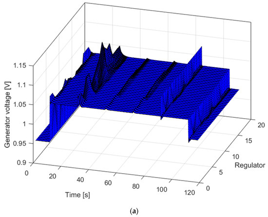
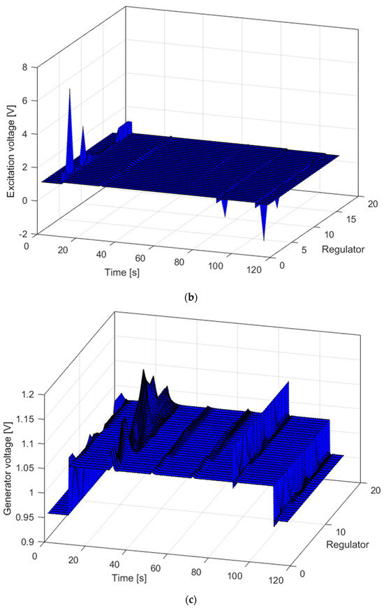
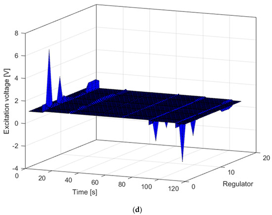
Figure 3.
Three-dimensional dependence: (a) generator voltage, time, and regulator for step changes of 5%, (b) excitation voltage, time, and regulator for step changes of 5%, (c) generator voltage, time, and regulator for step changes of 7%, (d) excitation voltage, time, and regulator for step changes of 7%.
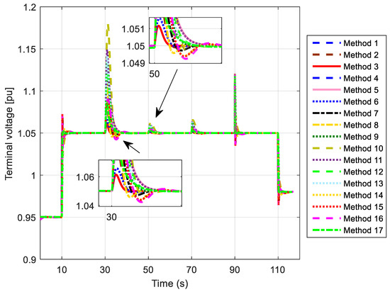
Figure 4.
Terminal voltage change versus time for all methods presented in Table 4.
Multiple conclusions can be drawn from Figure 3 and Figure 4. First, the observed scheme states that changing the generator voltage’s reference value is equivalent to adding a disturbance signal to the sensor’s output (but with an opposite sign). Based on the simulation findings that have been shown, this conclusion is obvious. Second, the interference at the amplifier and exciter outputs has a negligible impact on the generator’s output voltage responses. The additional signal at the output of the regulator, and the signal at the output of the generator voltage, produce a notable effect on the waveform of the generator voltage. According to the design, this signal is sent directly to the block output that describes the generator itself. This makes it easy to see how the interference affects the generator voltage. The differences between the results are very small, and they do not impact much in real life. However, they show that the proposed regulator type is accurate and that the proposed method can be used. A change in the signal at the generator output voltage substantially impacts the generator voltage’s reference value if the excitation voltage is under observation. Otherwise, it is crucial to remember that real systems cannot tolerate excitation voltage values with an indefinite range. In transitional systems, the excitation voltage is restricted to 3 pu, whereas the practical limits are 1.6 pu. Excitation voltages that are too high, over the maximum permitted value, may damage field windings and result in short circuits.
4. PSO–AVO Algorithm
At present, metaheuristic algorithms can be used to tackle many optimization challenges effectively. They are general-purpose algorithms that do not go beyond the initial settings. In this regard, this paper presents the application of a hybrid variant of two metaheuristic algorithms—the African vulture optimization (AVO) algorithm [29] and the particle swarm optimization (PSO) algorithm [14], named PSO–AVOA.
The PSO algorithm’s basic idea is to alter the speed and location of each variable iteratively. To find the current best position (in the current iteration) and the past best global positions (in all previous iterations), the distance of each variable is specifically evaluated during each iteration. In this regard, a randomly generated change value is used to be changed from one location to another.
Namely, let P and B represent vectors of current positions and current variable velocities, respectively:
The velocity and position of each variable in the next iteration are calculated as:
where Pmax and Pmin represent the predefined minimum and maximum value of the variables; C1, C2, and T are weight coefficients; pbest and qbest are the best current position and the best global position; rand1 and rand2 are randomly generated numbers from 0 to 1; Iter is the current iteration; Itermax is the maximum number of iterations; and Tmax and Tmin are the final (maximum) and initial (minimum) values of the weight coefficients. It should be emphasized that the coefficients C1 and C2 (the so-called acceleration factor) play a key role in determining how quickly convergence occurs. The convergence is slow if these coefficients have low values. The optimization process, however, may become unstable if their values are high [30]. The PSO procedure’s end values represent the starting values for the AVO algorithm. The main AVO algorithm uses these initial values, which are provided by the PSO. The AVO algorithm divides all populations into two groups, and the process comprises four steps. The initialization of every individual is the fundamental stage in any metaheuristic algorithm. In this stage, the PSO and AVO algorithms are combined, since the PSO algorithm’s final population value corresponds to the AVO algorithm’s initial population.
After this step, the next step is calculating the fitness value of all vultures. In this step, the division of vultures must also be realized—the vulture with the lowest fitness value is chosen to be the best vulture of the first group (marked as Best_Vulture_1), while the second-best vulture from the whole population is selected as the second group’s best vulture (marked as Best_Vulture_2). Also, in this step, it is necessary to randomly choose one of the best vultures from these two groups (this random vulture is denoted as R(i)):
Using a roulette wheel, pi represents the probability of selecting the best vulture from either the first or second group. With the formula L1 + L2 = 1, L1 and L2 are parameters that balance the global and local search.
The third step focuses on the vultures’ starvation. In this phase, the satiation rate F must be determined as follows:
where ite and max_ite represent the current iteration and the maximum number of iterations, respectively, z is a random number in the range [–1, 1], h is a random number in the range [−2, 2], and r1 is a random number between 0 and 1. If |F| ≥ 1, the algorithm enters the exploration phase; if |F| < 1, the algorithm enters the exploitation phase.
The fourth phase represents the exploration phase. The positions of the vultures are updated as follows:
where X is the vector coefficient and is calculated as follows X = 2∙rand, while randP1, rand2, and rand3 are random numbers in the range [0, 1]. Also, there are two possible phases of exploitation depending on |F|. If the value of |F| is between 0.5 and 1, the predefined parameter P2, which must be between 0 and 1, is used to choose the strategy as follows:
where the terms S1 and S2 are defined as follows:
If the value of |F| is less than 0.5, the AVO algorithm enters the second exploitation phase as follows:
where P3 is previously defined, and the terms A1 and A2 represent the accumulation of the vultures from two different groups over the food source.
while the Levy flight pattern is expressed to increase the effectiveness of the algorithm as follows:
where u and v are random numbers between 0 and 1, while β is a parameter set to 1.5.
The previously described sequence represents the entire AVO process. The algorithm repeats all these steps until the maximum number of iterations is reached. In Figure 5, the algorithm flowchart is presented.
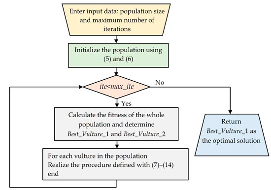
Figure 5.
Flowchart of the PSO–AVOA.
5. Simulation Results
Based on the modeling results in the third chapter, the key elements that change the generator voltage are the disturbance signal at the output of the regulator and the disturbance signal at the output of the generator block, after the step value of the generator voltage changes. On the other hand, due to practical restrictions, the excitation voltage must remain below a particular limit throughout all changes. The following objective function is developed in light of these observations.
The objective function has three parts if the excitation voltage is below a pre-determined maximum. The well-known Zwe-Lee Gaing objective function model of the objective function is represented in the first part, related to a change in step generator voltage reference. The step disturbance of the generator voltage change, and the regulator signal change, are represented in the second and third parts.
Both parts of the objective are specified as simple integrals of absolute error (IAE), as the goal is to neutralize the influence of these disruptions as fast as possible. On the other hand, if the excitation voltage value is greater than the predefined maximum in any time step, the objective function has an infinite value.
First, using the proposed objective function and all of the regulator parameters listed in Table 1—all derived from the literature—the value was determined for each regulator type. The results of applying this suggested objective function are shown in Figure 6, where the value of the proposed objective function was scaled to the highest value attained by the methods in the literature (in this case, Method #10 in [26] provides the highest value of the criterion function). In all the observed methods, it is clear that the methods presented in [25] provide the best results.
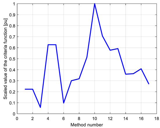
Figure 6.
Values of the criteria function for all methods provided in Table 4.
It is evident from Figure 6 that Methods #3 and #6 provide the highest-quality response and the lowest value of the objective function, respectively, with the PIDD2 regulator. Using the PIDD2 regulator ensures the best outcomes regarding the effectiveness of various step disturbances and the quality of the transition process. This work estimates the parameters of the PIDD2 regulator based on that finding.
Figure 7 and Figure 8 show the generator voltage response to the disturbances above, as well as the corresponding excitation voltage. As can be seen, Method #3 allows for the results to be obtained when the excitation voltage reaches its maximum value during the transition process and is more than 6 pu. Method #6 uses an excitation voltage that is at its highest value during the transition process—3.5 pu. Even though it is not safe or secure, the higher excitation voltage value during the transition process makes it possible for the generator voltage to respond more quickly. When the excitation voltage is within acceptable ranges, other methods can be used to get good results. However, the process of transitioning in these methods takes longer than the process taken using Methods #3 and #6.
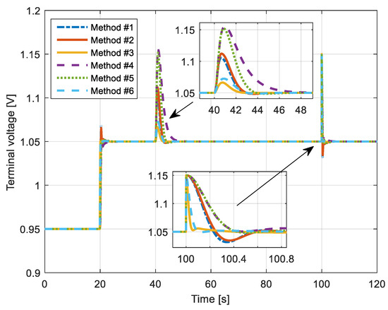
Figure 7.
Terminal voltage response for regulator parameters based on Methods #1–6 (in 20 s—the effects of generator voltage reference change, in 40 s—the impact of the additional signal on the regulator output, in 100 s—the impact of the additional signal on the generator output).
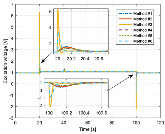
Figure 8.
Excitation voltage response for regulator parameters based on Methods #1–6 (in 20 s—the effects of generator voltage reference change, in 40 s—the impact of the additional signal on the regulator output, in 100 s—the impact of the additional signal on the generator output).
5.1. Regulator Parameter Estimation for Different Maximum Values of the Excitation Voltage
Applying the proposed algorithm, the PIDD2 regulator parameters are determined for the various maximum values of the excitation voltage based on the previously observed findings. The maximum value was explicitly determined to be 4 pu, 3.5 pu, 2.5 pu, 2 pu, and 1.6 pu. In other words, we used the same parameter limits as in the other works [3,4,5,6,7,8,9,10,11,12,13,14,15,16,17,18,19,20,21,22,23,24,25]. Table 5 lists the regulator’s determined parameters. As noted, the lower excitation voltage results in lower values for all regulator parameters. In [22], the same finding is shown for different types of regulators when it comes to how the excitation voltage value affects the regulator parameter values.
Table 5.
The estimated PIDD2 regulator parameters for different values of the excitation voltage.
In Figure 9, a comparison is shown between the generator voltage’s responses to variations in the generator reference voltage (20 s), the signals following the regulator (30 s), the amplifier (40 s), and the exciter (50 s) outputs, respectively. All the step disturbances are assumed to have a value of 0.1 pu. Figure 10 shows a comparison of the excitation voltage responses. The results made it abundantly evident that the lower value of the maximum excitation voltage ensures both safe and secure operation of the machine and, at the same time, the slowest response to any disturbances. It is also evident that the highest impact on the excitation voltage change causes the change of the generator reference voltage. However, the highest impact on the generator voltage is the signal added to the output of the regulator.
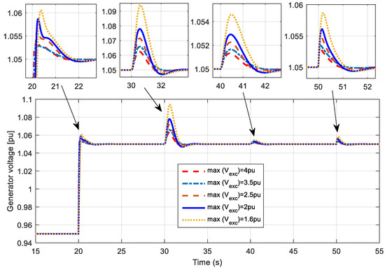
Figure 9.
Generator voltage responses with different disturbances (in 20 s—the effects of the generator voltage reference change, in 30 s—the impact of the additional signal on the regulator output, in 40 s—the impact of the additional signal on the amplifier output, in 50 s—the impact of the additional signal on the exciter output).
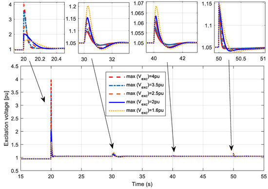
Figure 10.
Excitation voltage responses with different disturbances (in 20 s—the effects of the generator voltage reference change, in 30 s—the impact of the additional signal on the regulator output, in 40 s—the impact of the additional signal on the amplifier output, in 50 s—the impact of the additional signal on the exciter output).
5.2. Comparison of the Results Obtained with Different Literature Approaches
The proposed method for estimating the AVR regulator parameters is justified by comparing the results to those found in the literature, as illustrated in Figure 11 and Figure 12. In particular, it is evident from the results presented in the previous sections that Method #6 provides the generator voltage response when the excitation voltage is at its maximum value of 3.5 pu. We compared the generator and excitation voltage response simulation results in the scenario where the maximum excitation voltage is 3.5 pu.
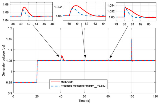
Figure 11.
Generator voltage responses with different disturbances (in 20 s—the effects of the generator voltage reference change; in 40 s—the impact of the additional signal on the regulator output; in 60 s—the impact of the additional signal on the amplifier output; in 80 s—the impact of the additional signal on the exciter output; in 100 s—the impact of the additional signal on the generator output).
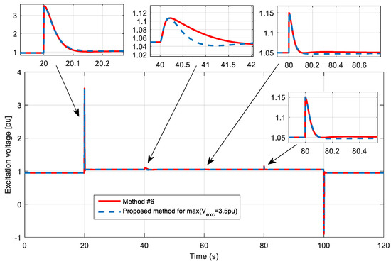
Figure 12.
Excitation voltage responses with different disturbances (in 20 s—the effects of the generator voltage reference change; in 40 s—the impact of the additional signal on the regulator output; in 60 s—the impact of the additional signal on the amplifier output; in 80 s—the impact of the additional signal on the exciter output; in 100 s—the impact of the additional signal on the generator output).
It is clearly apparent from the results that the suggested method outperforms the existing methods in the literature, in terms of effectiveness, speed, and neutrality of action of disturbances from the regulator, the amplifiers, and the exciter.
Using a novel method for estimating the parameters of the AVR regulator structure has a clear justification in light of the investigations presented. Additionally, it is evident, by looking at the value of the criteria function, that the outcomes obtained through the suggested methods are superior to those provided by Method #6 in terms of the objective function. In a scaled form, the corresponding results of the proposed method and Method #6 are shown in Figure 13.
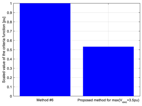
Figure 13.
Comparison of the objective function value obtained by the proposed method and Method #6.
Finally, we compared the response of the generator voltage in the case of applying a step change on the reference value of the generator voltage, as well as changes in the signal at the output of the regulator, changes in the signal at the output of the amplifier, changes in the signal at the output from the exciter, and changes in the signal at the output from the generator voltage; the parameters being obtained by applying the literature methods described in [5,25], with the results being obtained using the proposed method using the parameters determined, with a maximum excitation voltage of 3.5 pu. As demonstrated by the results, the parameters derived from the proposed method enable the speediest elimination of step changes, the generator voltage reference value, and signal changes at the regulator’s output. This is most evident in the zoomed portions of the displayed figures. There is no doubt that this method yields the shortest settling time. Conversely, the value of the criterion function is also the smallest, as shown in Figure 14, confirming that the proposed method is accurate.
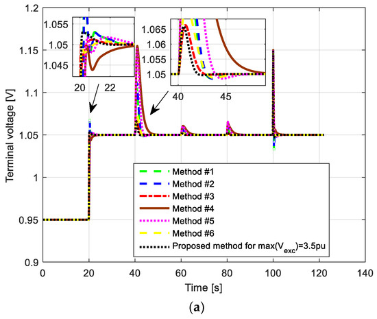
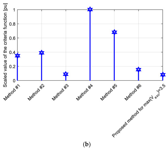
Figure 14.
Comparison of the results obtained with literature methods presented in [5,25]: (a) terminal voltage change versus time, and (b) scaled objective functions.
5.3. Robustness Analysis
While analyzing the robustness of the proposed AVR parameters, the effect of altering the parameter values of the synchronous machines is observed. In other words, the gain and time constant fluctuate based on the load value. In order to achieve this, the values of the rise time, settling time, and overshoot, as well as the IAE values, are measured when the generator voltage reference changes and when the regulator output signal and the generator output signal change, respectively. The simulation step was assumed to be 10−4, and the values of all changes were assumed to be 0.1 pu. The maximum allowed excitation voltage values are shown in Table 6 for all parameters set for all values. Figure 15 and Figure 16 show the excitation voltage and the generator voltage for the maximum excitation voltage of 1.6 pu and various generator gain and time constant values. Based on the results, it is evident that the suggested approach (controller and parameters) ensures the system’s robustness to changes in the characteristics of the synchronous machines.
Table 6.
Investigating the impact of synchronous machine gain and time constant changes on the characteristic’s response value.
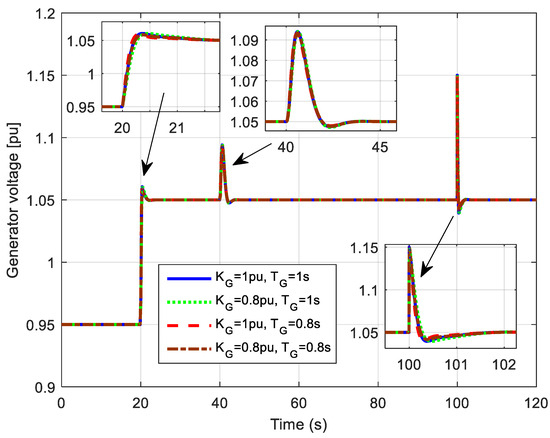
Figure 15.
Generator voltage responses with different disturbances for a maximum excitation voltage of 1.6 pu (in 20 s—the effects of the generator voltage reference change, in 40 s—the impact of the additional signal on the regulator output, in 100 s—the impact of the additional signal on the generator output).
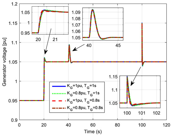
Figure 16.
Excitation voltage responses with different disturbances for a maximum excitation voltage of 1.6 pu (in 20 s—the effects of the generator voltage reference change, in 40 s—the impact of the additional signal on the regulator output, in 100 s—the impact of the additional signal on the generator output).
5.4. Proposed Algorithm Tests
Finally, the effectiveness of the proposed algorithm is tested from the perspectives of convergence curves and statistical findings to confirm the rationale for its implementation. The test is run assuming that max Vexc = 4 pu.
A 3D graph convergence curve resulting from the proposed method, which was initiated 30 times with 50 iterations between each start, is shown in Figure 17. As illustrated in Figure 18, the Chaotic AVOA, PSO–AVOA, and the standard AVOA compare the mean value and the convergence curve. The statistical processing of findings in the form of maximum, minimum, and mean values, and the comparison in terms of Wilcoxon’s rank-sum test, were carried out based on the provided results and numerous tests of each algorithm stated (Table 7).
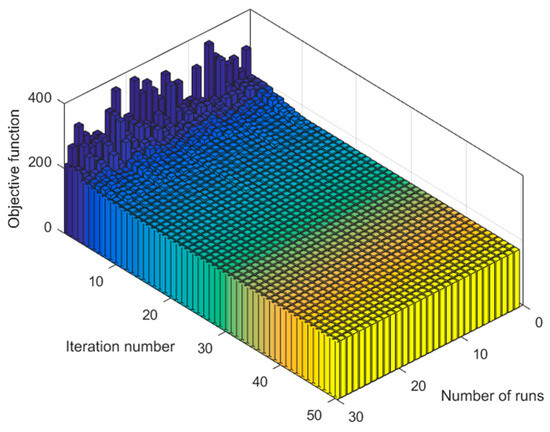
Figure 17.
A 3D view of the objective function value, number of iterations, and runs.
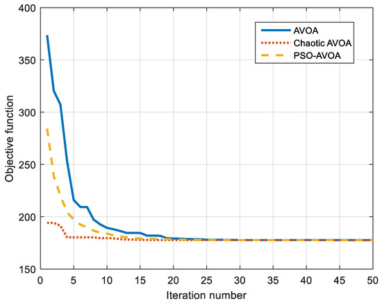
Figure 18.
Mean convergence curves of the different investigated algorithms.
Table 7.
Comparison of the results obtained with the different investigated algorithms, in terms of the statistical measures and p-values obtained with Wilcoxon’s rank-sum test.
The proposed algorithm guarantees the best outcomes in terms of speed and convergence statistical tests. As a result, the suggested algorithm’s applicability, effectiveness, and rapid convergence are presented and discussed.
6. Conclusions
This paper deals with the design of the regulator for the automatic voltage regulation system of synchronous machines. However, in contrast to previous literature’s approaches, this work considers the AVR scheme, where interference signals are added to each element. A 6ISO system was proposed in this manner. Analyzing the response of the generator voltage when using different types of regulators whose parameters are designed using different methods in the literature, it was observed that the dominant effects on the output voltage of the generator are interference on the regulator signal and interference on the generator voltage with a step change in the reference value of the generator voltage. The simulations also show that the generator voltage output form is not significantly affected by changes in the output from the excitation or by changes in the signal from the amplifier.
A new objective function was defined in light of the previously mentioned findings. The research also suggests using a novel metaheuristic algorithm that merges one of the more recent AVO metaheuristic algorithms with the well-known PSO algorithm. The regulator settings were calculated using the suggested hybrid technique in limited and unlimited excitation voltage cases.
Based on the results, it was determined that the suggested algorithm provides results superior to those found in the literature and converges noticeably quicker. As a result, the response and voltage of the generator are improved. Future research will focus on developing novel types, i.e., regulator structures incorporating filter components in the sensor branch and the practical implementation of various regulator structures in synchronous machines.
Author Contributions
Conceptualization, M.C., M.M. and S.H.E.A.A.; methodology, M.C.; validation, M.R., S.A. (Sultan Alghamdiand), O.A., and S.A. (Salem Alkhalaf); formal analysis, S.A. (Sultan Alghamdiand) and Z.M.A.; investigation, M.C.; resources, S.A. (Sultan Alghamdiand), M.R., O.A., Z.M.A. and S.A. (Salem Alkhalaf); data curation, M.C. and S.H.E.A.A.; writing—original draft preparation, M.M. and M.C.; writing—review and editing, S.H.E.A.A.; visualization, M.C. and S.H.E.A.A.; funding, M.R. and S.A. (Sultan Alghamdiand). All authors have read and agreed to the published version of the manuscript.
Funding
This research received no external funding.
Data Availability Statement
Not applicable.
Conflicts of Interest
The authors declare no conflict of interest.
References
- Boldea, I. Synchronous Generators, 2nd ed.; CRC Press: Boca Raton, FL, USA, 2016. [Google Scholar]
- Nadeem, M.; Imran, K.; Khattak, A.; Ulasyar, A.; Pal, A.; Zeb, M.Z.; Khan, A.N.; Padhee, M. Optimal Placement, Sizing and Coordination of FACTS Devices in Transmission Network Using Whale Optimization Algorithm. Energies 2020, 13, 753. [Google Scholar] [CrossRef]
- Sikander, A.; Thakur, P. A New Control Design Strategy for Automatic Voltage Regulator in Power System. ISA Trans. 2020, 100, 235–243. [Google Scholar] [CrossRef] [PubMed]
- Ekinci, S.; Hekimoglu, B. Improved Kidney-Inspired Algorithm Approach for Tuning of PID Controller in AVR System. IEEE Access 2019, 7, 39935–39947. [Google Scholar] [CrossRef]
- Micev, M.; Ćalasan, M.; Ali, Z.M.; Hasanien, H.M.; Abdel Aleem, S.H.E. Optimal design of automatic voltage regulation controller using hybrid simulated annealing—Manta ray foraging optimization algorithm. Ain Shams Eng. J. 2021, 12, 641–657. [Google Scholar] [CrossRef]
- Sikander, A.; Thakur, P.; Bansal, R.C.; Rajasekar, S. A novel technique to design cuckoo search-based FOPID controller for AVR in power systems. Comput. Electr. Eng. 2018, 70, 261–274. [Google Scholar] [CrossRef]
- Ortiz-Quisbert, M.E.; Duarte-Mermoud, M.A.; Milla, F.; Castro-Linares, R.; Lefranc, G. Optimal fractional-order adaptive controllers for AVR applications. Electr. Eng. 2018, 100, 267–283. [Google Scholar] [CrossRef]
- Mosaad, A.M.; Attia, M.A.; Abdelaziz, A.Y. Whale optimization algorithm to tune PID and PIDA controllers on AVR system. Ain Shams Eng. J. 2019, 10, 755–767. [Google Scholar] [CrossRef]
- Sahib, M.A. A novel optimal PID plus second-order derivative controller for AVR system. Eng. Sci. Technol. Int. J. 2015, 18, 194–206. [Google Scholar] [CrossRef]
- Panda, S.; Sahu, B.K.; Mohanty, P.K. Design and performance analysis of PID controller for an automatic voltage regulator system using simplified particle swarm optimization. J. Frankl. Inst. 2012, 349, 2609–2625. [Google Scholar] [CrossRef]
- Zhang, D.-L.; Tang, Y.-G.; Guan, X.-P. Optimum Design of Fractional Order PID Controller for an AVR System Using an Improved Artificial Bee Colony Algorithm. Acta Autom. Sin. 2014, 40, 973–979. [Google Scholar] [CrossRef]
- Mosaad, A.M.; Attia, M.A.; Abdelaziz, A.Y. Comparative Performance Analysis of AVR Controllers Using Modern Optimization Techniques. Electr. Power Compon. Syst. 2018, 46, 2117–2130. [Google Scholar] [CrossRef]
- Gozde, H.; Taplamacioglu, M.C. Comparative performance analysis of artificial bee colony algorithm for automatic voltage regulator (AVR) system. J. Frankl. Inst. 2011, 348, 1927–1946. [Google Scholar] [CrossRef]
- Gaing, Z.L. A particle swarm optimization approach for optimum design of PID controller in AVR system. IEEE Trans. Energy Convers. 2004, 19, 384–391. [Google Scholar] [CrossRef]
- Rais, M.C.; Dekhandji, F.Z.; Recioui, A.; Rechid, M.S.; Djedi, L. Comparative Study of Optimization Techniques Based PID Tuning for Automatic Voltage Regulator System. Eng. Proc. 2022, 14, 21. [Google Scholar] [CrossRef]
- Micev, M.; Ćalasan, M.; Oliva, D. Fractional-order PID controller design for an AVR system using Chaotic Yellow Saddle Goatfish Algorithm. Mathematics 2020, 8, 1182. [Google Scholar] [CrossRef]
- Chatterjee, S.; Mukherjee, V. PID controller for automatic voltage regulator using teaching–learning-based optimization technique. Int. J. Electr. Power Energy Syst. 2016, 77, 418–429. [Google Scholar] [CrossRef]
- Ayas, M.S.; Sahin, E. FOPID controller with fractional filter for an automatic voltage regulator. Comput. Electr. Eng. 2021, 90, 106895. [Google Scholar] [CrossRef]
- Elsisi, M.; Tran, M.Q.; Hasanien, H.M.; Turky, R.A.; Albalawi, F.; Ghoneim, S.S.M. Robust model predictive control paradigm for automatic voltage regulators against uncertainty based on optimization algorithms. Mathematics 2021, 9, 2885. [Google Scholar] [CrossRef]
- Tang, Y.; Cui, M.; Hua, C.; Li, L.; Yang, Y. Optimum design of fractional-order PIλDμ controller for AVR system using chaotic ant swarm. Expert Syst. Appl. 2012, 39, 6887–6896. [Google Scholar] [CrossRef]
- Tang, Y.; Zhao, L.; Han, Z.; Bi, X.; Guan, X. Optimal gray PID controller design for automatic voltage regulator system via imperialist competitive algorithm. Int. J. Mach. Learn. Cybern. 2016, 7, 229–240. [Google Scholar] [CrossRef]
- Ćalasan, M.; Micev, M.; Radulović, M.; Zobaa, A.F.; Hasanien, H.M.; Abdel Aleem, S.H.E. Optimal PID controllers for AVR system considering excitation voltage limitations using hybrid equilibrium optimizer. Machines 2021, 9, 265. [Google Scholar] [CrossRef]
- Hasanien, H.M. Design Optimization of PID Controller in Automatic Voltage Regulator System Using Taguchi Combined Genetic Algorithm Method. IEEE Syst. J. 2013, 7, 825–831. [Google Scholar] [CrossRef]
- Blondin, M.J.; Sanchis, J.; Sicard, P.; Herrero, J.M. New optimal controller tuning method for an AVR system using a simplified Ant Colony Optimization with a new constrained Nelder–Mead algorithm. Appl. Soft Comput. 2018, 62, 216–229. [Google Scholar] [CrossRef]
- Alghamdi, S.; Sindi, H.F.; Rawa, M.; Alhussainy, A.A.; Ćalasan, M.; Micev, M.; Ali, Z.M.; Abdel Aleem, S.H.E. Optimal PID Controllers for AVR Systems Using Hybrid Simulated Annealing and Gorilla Troops Optimization. Fractal Fract. 2022, 6, 682. [Google Scholar] [CrossRef]
- Blondin, M.J.; Sicard, P.; Pardalos, P.M. Controller Tuning approach with robustness, stability, and dynamic criteria for the original AVR System. Math. Comput. Model. 2019, 163, 168–182. [Google Scholar] [CrossRef]
- Bingul, Z.; Karahan, O. A novel performance criterion approach to the optimum design of PID controller using cuckoo search algorithm for AVR system. J. Frankl. Inst. 2018, 355, 5534–5559. [Google Scholar] [CrossRef]
- Çelik, E.; Durgut, R. Performance enhancement of automatic voltage regulator by modified cost function and symbiotic organisms search algorithm. Int. J. Eng. Sci. Technol. 2018, 21, 1104–1111. [Google Scholar] [CrossRef]
- Abdollahzadeh, B.; Gharehchopogh, F.S.; Mirjalili, S. African vultures optimization algorithm: A new nature-inspired metaheuristic algorithm for global optimization problems. Comput. Ind. Eng. 2021, 158, 107408. [Google Scholar] [CrossRef]
- Sakthivel, V.P.; Bhuvaneswari, R.; Subramanian, S. Multiobjective parameter estimation of induction motor using particle swarm optimization. Eng. Appl. Artif. Intell. 2010, 23, 302–312. [Google Scholar] [CrossRef]
Disclaimer/Publisher’s Note: The statements, opinions and data contained in all publications are solely those of the individual author(s) and contributor(s) and not of MDPI and/or the editor(s). MDPI and/or the editor(s) disclaim responsibility for any injury to people or property resulting from any ideas, methods, instructions or products referred to in the content. |
© 2023 by the authors. Licensee MDPI, Basel, Switzerland. This article is an open access article distributed under the terms and conditions of the Creative Commons Attribution (CC BY) license (https://creativecommons.org/licenses/by/4.0/).