Modeling and Dynamical Analysis of a Fractional-Order Predator–Prey System with Anti-Predator Behavior and a Holling Type IV Functional Response

Abstract

We here investigate the dynamic behavior of continuous and discrete versions of a fractional-order predator–prey system with anti-predator behavior and a Holling type IV functional response. First, we establish the non-negativity, existence, uniqueness and boundedness of solutions to the system from a mathematical analysis perspective. Then, we analyze the stability of its equilibrium points and the possibility of bifurcations using stability analysis methods and bifurcation theory, demonstrating that, under specific parameter conditions, the continuous system exhibits a Hopf bifurcation, while the discrete version exhibits a Neimark–Sacker bifurcation and a period-doubling bifurcation. After providing numerical simulations to illustrate the theoretically derived conclusions and by summarizing the various analytical results obtained, we finally present four interesting conclusions that can contribute to better management and preservation of ecological systems.

1. Introduction

The study of predator–prey systems can be traced back to the 18th century. However, the establishment of predator–prey systems in the modern sense is primarily attributed to the work of Alfred J. Lotka and Vito Volterra in the early 20th century. They independently proposed models for predator–prey systems and conducted in-depth research on their dynamical behavior. Their research laid an important theoretical foundation for the dynamics of predator–prey systems. Lotka–Volterra systems describe the interactions between predator and prey, and quickly became a hot topic in dynamical research. Even today, studying the dynamical relationship between predator and prey remains an important subject. To comprehend the intricate dynamical properties presented in predator–prey systems, numerous researchers have dedicated themselves to studying predator–prey models in depth. During the course of their research, they have found multitudes of fascinating dynamical properties among various systems. Berryman [1] pointed out that the original Lotka–Volterra predator–prey equations were built around the principle of mass action, and equations derived in this way lead to the paradoxes of enrichment and biological control. Wang and Chen [2] established the condition for the permanence of populations and sufficient conditions under which positive equilibrium of the model is globally stable. References [3,4] investigated the complex dynamical behavior of discrete predator–prey systems. Qi and Meng [5] found that in a predator–prey system with prey refuge and the fear effect, the survival rate of prey can be improved by increasing the strength of the refuge, decreasing the cost of fear or reducing the intensity of white noise. Blasius, Rudolf, et al. [6] found through experiments that a long-term cyclic persistence exists in a simple predator–prey model. Mukherjee [7] and Qiu and Guo [8] investigated the complex dynamics of a predator–prey system with the fear effect and a predator–prey system with prey taxis, respectively. Although we may subconsciously assume that prey are inherently disadvantaged in a predator–prey system, there are many instances where prey can resist predation and cause harm to predators, even leading to the death of the predator. The existence of such scenarios underscores the significance of determining which entities hold the advantage of prey in a predator–prey system [9].

The anti-predator behavior of prey is widely observed in the natural world. Many scholars have conducted research on the anti-predator behavior of prey and have identified two main ways in which prey exhibit such behaviors: (1) through morphological or behavioral changes [10,11], or (2) by actively attacking the predator [12,13,14].

In 1987, Ives and Dobson [15] proposed the following system to simulate anti-predator behavior (1):

$$\left\{\begin{array}{c}\frac{dx}{dt}=\alpha x\left(1-\frac{x}{k}\right)-\beta -\frac{e^{-\gamma \beta }qxy}{1+ax},\hfill \\ \frac{dy}{dt}=\frac{b{e}^{-\gamma \beta }qxy}{1+ax}-dy,\hfill \end{array}\right.$$

(1.1)

where the meanings of all parameters are presented in Table 1.

Table 1. Biological meanings of all parameters in system (1.1).

Parameter	Meaning
x	Prey population density
y	Predator population density
$\alpha >0$	Natality of prey population
$k>0$	Carrying capacity of the environment to prey
$\beta >0$	Cost incurred by the prey as a result of anti-predator behavior
$\gamma >0$	Effects resulting from the anti-predator behavior of prey
$\frac{qx}{1+ax},q>0,a>0$	Holling II functional response function
$b>0$	Conversion rate of prey consumed by predator
$d>0$	Death rate of predator population

The prey requirements in anti-predator behavior (2) are higher, as they not only demand that adult prey can resist predation by predators but also require adult prey to have the ability to kill the juveniles of the predator. However, there have been few studies on anti-predator behavior (2). In 2015, Tang and Xiao [16] proposed a system to simulate anti-predator behavior (2), and considered the following Holling type IV functional response function system:

$$\left\{\begin{array}{c}\frac{du}{dt}=au\left(1-\frac{u}{k}\right)-\frac{buv}{h+u^2},\hfill \\ \frac{dv}{dt}=\frac{cbuv}{h+u^2}-dv-guv,\hfill \end{array}\right.$$

(1.2)

where the meanings of all parameters are given in Table 2. It is worth noting that the Holling type IV functional response function used in this paper was originally proposed by W. Sokol [17] and has been widely applied in predator–prey systems for several decades. It primarily describes a nonlinear interaction between a predator and its prey. The predation rate of the predator adjusts to changes in the population density of prey, exhibiting a saturation tendency.

Table 2. Biological meanings of parameters in systems (1.2) and (1.3).

Parameter	Meaning
u	Prey population density
v	Predator population density
$a>0$	Natality of prey population
$k>0$	Carrying capacity of the environment to prey
$b>0$	Predator’s capture rate
$c>0$	Conversion rate of prey into predator
$\frac{bu}{h+u^2},h>0$	Holling type IV functional response function
$d>0$	Death rate of predator
$g>0$	Mortality rate of predator due to the anti-predator effects of prey
$0<\alpha \le 1$	Order of fractional-order derivative

The concept of fractional derivatives can be traced back to the 18th century, and the mathematician who first proposed fractional derivatives was Liouville [18]. In the 20th century, the mathematician Riesz made the initial reference to the concept of fractional derivatives and conducted research on their properties in reference [19], combining the studies of Liouville and Riesz to establish the Riesz–Liouville definition of fractional derivatives that is used today. Subsequently, the mathematician Caputo introduced the Caputo definition of fractional derivatives in reference [20].

Definition 1. 

Denote

$${}_0^C{D}_t^{\alpha }f\left(t\right)=J^{l-\alpha }{f}^{\left(l\right)}\left(t\right),\alpha >0,$$

where $f^{\left(l\right)}$ denotes the derivative of f with order l, l is the nearest integer value of α, and $J^q$ is the operator of the Riemann–Liouville integral of q order:

$$J^{q}h\left(t\right)=\frac{{\int }_0^t{(t-{\tau }_e)}^{q-1}h\left({\tau }_e\right)d{\tau }_e}{\mathrm{\Gamma }\left(q\right)},$$

where $\mathrm{\Gamma }\left(q\right)$ is Euler’s Gamma function. The $alpha$-order Caputo differential operator is the term used to describe the operator ${}_0^C{D}_t^{\alpha }$.

From a biological perspective, considering a fractional-order predator–prey system makes logical sense; for most organisms in the natural world, their current behaviors are influenced by historical context. In fractional calculus, the rate of change at any given moment, i.e., the fractional-order derivative, depends on the population density over a certain period of time. Therefore, fractional-order predator–prey systems have unique advantages in describing memory effects within populations. Over the past two decades, owing to the advantages of fractional derivatives in studying various ecological systems’ memory effects, numerous mathematicians have turned their attention to investigating fractional-order ecological systems, finding many interesting dynamical properties presented in them [21,22,23,24,25,26,27,28]. At present, a relatively comprehensive research framework has been established for mathematical models of integer-order ecosystems, while the study of fractional-order ecosystems is still in its early stages. Hence, the authors of this paper intend to introduce the Caputo fractional derivation to system (1.2) and extend it to a fractional-order ecosystem. We intend to employ the Caputo definition of fractional derivatives to analyze how anti-predator behavior and the Holling type IV functional response function in a fractional-order ecosystem will impact the dynamics of the system. As a result, we introduce the following fractional-order predator–prey system with a Holling type IV functional response and anti-predator behaviors:

$$\left\{\begin{array}{c}{}_0^C{D}_t^{\alpha }u\left(t\right)=au\left(1-\frac{u}{k}\right)-\frac{buv}{h+u^2},\hfill \\ {}_0^C{D}_t^{\alpha }v\left(t\right)=\frac{cbuv}{h+u^2}-dv-guv,\hfill \end{array}\right.$$

(1.3)

where the meanings of all parameters are presented in Table 2. For the method of introducing the Caputo fractional differential equation into an ecosystem model, reference [29] may be consulted.

There is a current lack of comprehensive dynamic analysis methods for continuous fractional-order predator–prey systems. For example, in the literature [30], the analysis of fractional-order systems has mainly focused on Hopf bifurcations, while more extensive research has been dedicated to analyzing integer-order cases.

In references [31,32], the authors, respectively, conducted dynamical analyses of different discretized predator–prey models and found that discrete predator–prey models, in comparison to their continuous counterparts, exhibit a greater variety of dynamical behaviors and hold advantages in numerical simulations. In reference [33], the authors employed the piecewise constant approximation (PCA) method to discretize a continuous fractional-order predator–prey system and analyzed the dynamical properties of and discussed the types of bifurcations present in this system. Their work motivates us to consider the discrete counterpart of system (1.3). In recent years, many researchers have studied the dynamical behavior of discrete fractional-order predator–prey systems and have discovered numerous intriguing dynamical properties within these systems [34,35,36].

Hence, in order to better understand the properties of system (1.3), we here also consider discretizing system (1.3) for further dynamical analyses and comparing its properties with the continuous model (1.3), finding that there are many differences in dynamical properties between system (1.3) and its discrete version (1.6). This sufficiently shows that it is very helpful to consider the same problems from different angles.

We use the PCA method to discretize model (1.3), and the specific steps are as follows:

Assume that the initial conditions of system (1.3) are $u\left(0\right)=u_0$ and $v\left(0\right)=v_0$. The discretized version of model (1.3) is given as

$$\left\{\begin{array}{c}{}_0^C{D}_t^{\alpha }u\left(t\right)=au\left(\left[\frac{t}{\rho }\right]\right)(1-\frac{u\left(\left[\frac{t}{\rho }\right]\right)}{k})-\frac{bu\left(\left[\frac{t}{\rho }\right]\right)v\left(\left[\frac{t}{\rho }\right]\right)}{h+u{\left(\left[\frac{t}{\rho }\right]\right)}^2},\hfill \\ {}_0^C{D}_t^{\alpha }v\left(t\right)=\frac{cbu\left(\left[\frac{t}{\rho }\right]\right)v\left(\left[\frac{t}{\rho }\right]\right)}{h+u{\left(\left[\frac{t}{\rho }\right]\right)}^2}-dv\left(\left[\frac{t}{\rho }\right]\right)-gu\left(\left[\frac{t}{\rho }\right]\right)v\left(\left[\frac{t}{\rho }\right]\right).\hfill \end{array}\right.$$

First, let $t\in [0,\rho )$, then $\frac{t}{\rho }\in [0,1)$. Thus, we obtain

$$\left\{\begin{array}{c}{}_0^C{D}_t^{\alpha }u\left(t\right)=a{u}_0\left(1-\frac{u_0}{k}\right)-\frac{b{u}_0{v}_0}{h+u_0^2},\hfill \\ {}_0^C{D}_t^{\alpha }v\left(t\right)=\frac{cb{u}_0{v}_0}{h+u_0^2}-d{v}_0-g{u}_0{v}_0.\hfill \end{array}\right.$$

(1.4)

The answer to (1.4) is simplified to

$$\begin{array}{cc}\hfill u_1\left(t\right)& =u_0+J^{\alpha }(a{u}_0(1-\frac{u_0}{k})-\frac{b{u}_0{v}_0}{h+u_0^2})\hfill \\ \hfill & =u_0+\frac{t^{\alpha }}{\alpha \mathrm{\Gamma }\left(\alpha \right)}(a{u}_0(1-\frac{u_0}{k})-\frac{b{u}_0{v}_0}{h+u_0^2}),\hfill \\ \hfill v_1\left(t\right)& =v_0+J^{\alpha }(\frac{cb{u}_0{v}_0}{h+u_0^2}-d{v}_0-g{u}_0{v}_0)\hfill \\ \hfill & =v_0+\frac{t^{\alpha }}{\alpha \mathrm{\Gamma }\left(\alpha \right)}(\frac{cb{u}_0{v}_0}{h+u_0^2}-d{v}_0-g{u}_0{v}_0).\hfill \end{array}$$

Second, let $t\in [\rho ,2\rho )$, so $\frac{t}{\rho }\in [1,2)$. Then,

$$\left\{\begin{array}{c}{}_0^C{D}_t^{\alpha }u\left(t\right)=a{u}_1\left(1-\frac{u_1}{k}\right)-\frac{b{u}_1{v}_1}{h+u_1^2},\hfill \\ {}_0^C{D}_t^{\alpha }v\left(t\right)=\frac{cb{u}_1{v}_1}{h+u_1^2}-d{v}_1-g{u}_1{v}_1.\hfill \end{array}\right.$$

(1.5)

After simplifying (1.5), we can obtain the following solution

$$\begin{array}{cc}\hfill u_1\left(t\right)& =u_1\left(\rho \right)+J_{\rho }^{\alpha }(a{u}_1(1-\frac{u_1}{k})-\frac{b{u}_1{v}_1}{h+u_1^2})\hfill \\ \hfill & =u_1\left(\rho \right)+\frac{{(t-\rho )}^{\alpha }}{\alpha \mathrm{\Gamma }\left(\alpha \right)}(a{u}_1(1-\frac{u_1}{k})-\frac{b{u}_1{v}_1}{h+u_1^2}),\hfill \\ \hfill v_1\left(t\right)& =v_1\left(\rho \right)+J_{\rho }^{\alpha }(\frac{cb{u}_1{v}_1}{h+u_1^2}-d{v}_1-g{u}_1{v}_1)\hfill \\ \hfill & =v_1\left(\rho \right)+\frac{{(t-\rho )}^{\alpha }}{\alpha \mathrm{\Gamma }\left(\alpha \right)}(\frac{cb{u}_1{v}_1}{h+u_1^2}-d{v}_1-g{u}_1{v}_1),\hfill \end{array}$$

where $J_{\rho }^{\alpha }=\frac{1}{\mathrm{\Gamma }\left(\alpha \right)}{\int }_{\rho }^t{(t-{\tau }_e)}^{\alpha -1}d{\tau }_e$, $0<\alpha <1$. After n repetitions, we obtain

$$\begin{array}{cc}\hfill u_{n+1}\left(t\right)& =u_n\left(n\rho \right)+\frac{{(t-n\rho )}^{\alpha }}{\alpha \mathrm{\Gamma }\left(\alpha \right)}(a{u}_n\left(n\rho \right)(1-\frac{u_n\left(n\rho \right)}{k})-\frac{b{u}_n\left(n\rho \right)v_n\left(n\rho \right)}{h+u_n{\left(n\rho \right)}^2}),\hfill \\ \hfill v_{n+1}\left(t\right)& =v_n\left(n\rho \right)+\frac{{(t-n\rho )}^{\alpha }}{\alpha \mathrm{\Gamma }\left(\alpha \right)}(\frac{cb{u}_n\left(n\rho \right)v_n\left(n\rho \right)}{h+u_n{\left(n\rho \right)}^2}-d{v}_n\left(n\rho \right)-g{u}_n\left(n\rho \right)v_n\left(n\rho \right)),\hfill \end{array}$$

where $t\in [n\rho ,(n+1\left)\rho \right)$. For $t\to (n+1)\rho ,$ the system above becomes

$$\begin{array}{c}\hfill \left\{\begin{array}{c}{u}_{n+1}=u_n+\frac{{\left(\rho \right)}^{\alpha }}{\mathrm{\Gamma }(\alpha +1)}\left(a{u}_n\left(1-\frac{u_n}{k}\right)-\frac{b{u}_n{v}_n}{h+u_n^2}\right),\hfill \\ v_{n+1}=v_n+\frac{{\left(\rho \right)}^{\alpha }}{\mathrm{\Gamma }(\alpha +1)}\left(\frac{cb{u}_n{v}_n}{h+u_n^2}-d{v}_n-g{u}_n{v}_n\right).\hfill \end{array}\right.\end{array}$$

(1.6)

The overall structure of this paper is described as follows: In Section 2, some preliminaries are provided for some definitions, lemmas and theorems that will be used to analyze the dynamical properties of systems (1.3) and (1.6). In Section 3, the well-posedness of system (1.3) is analyzed. In Section 4, the existence and stability of the equilibrium points of systems (1.3) and (1.6) are investigated, respectively. In Section 5, we demonstrate that, under certain parameter conditions, system (1.3) exhibits a Hopf bifurcation, while system (1.6) exhibits a Neimark–Sacker bifurcation and a period-doubling bifurcation. In Section 6, numerical simulations are performed to validate the results of our theoretical analysis. In Section 7, interesting conclusions are drawn based on some findings in the previous sections.

2. Preliminaries

In this section, we primarily introduce the definition and some conclusions of Caputo fractional derivatives that are necessary for our subsequent research.

Definition 2 

([37]). Under the definition of Caputo fractional derivatives, the fractional derivative of function $f\left(\xi \right)\in A{C}^n([0,+\infty ],\mathbb{R})$ is given as

$${}_0^C{D}_{\xi }^{\alpha }f\left(\xi \right)={\int }_0^{\xi }\frac{f^{\left(n\right)}\left(\vartheta \right)}{\mathrm{\Gamma }(n-\alpha ){(\xi -\vartheta )}^{\alpha -n+1}}d\vartheta ,$$

where α represents the order of the fractional derivative.

When $n=1$, the fractional derivative ${}_0^C{D}_{\xi }^{\alpha }f\left(\xi \right)$ takes the form of

$${}_0^C{D}_{\xi }^{\alpha }f\left(\xi \right)={\int }_0^{\xi }\frac{f\left(\vartheta \right)}{\mathrm{\Gamma }(1-\alpha ){(\xi -\vartheta )}^{\alpha }}d\vartheta .$$

Definition 3 

([37]). The Mittag–Leffler function $M_i$, when the order i of $M_i$ is positive, is defined as

$$M_i\left(\zeta \right)=\sum _{j=0}^{\infty }\frac{{\zeta }_j}{\mathrm{\Gamma }(ji+1)},{\zeta }_j\in \mathbb{C},$$

as the sequence converges.

Definition 4 

([38]). Let $Q(u,v)$ be a fixed piont of system (1.6) with multipliers ${\lambda }_1$ and ${\lambda }_2$.

$\left(i\right)$ If $|{\lambda }_1|<1$ and $|{\lambda }_2|<1$, the fixed point $Q(u,v)$ is called a sink, and the sink is locally asymptotically stable.

$\left(ii\right)$ If $|{\lambda }_1|>1$ and $|{\lambda }_2|>1$, the fixed point $Q(u,v)$ is called a source, and the source is locally asymptotically unstable.

$\left(iii\right)$ If $|{\lambda }_1|<1$ and $|{\lambda }_2|>1$(or $|{\lambda }_1|>1$ and $|{\lambda }_2|<1$), the fixed point $Q(u,v)$ is called a saddle.

$\left(iv\right)$ If either $|{\lambda }_1|=1$ or $|{\lambda }_2|=1$, the fixed point $Q(u,v)$ is called non-hyperbolic.

Lemma 1 

([39]). For ${}_0^C{D}_{\xi }^{\alpha }f\left(\xi \right)\in AC([0,\Xi ],\mathbb{R})$, if $f\left({\xi }_1\right)=0$ and $f\left({\xi }_0\right)>0$ (all ${\xi }_0\in [0,{\xi }_1))$, then ${}_0^C{D}_{\xi }^{\alpha }f\left({\xi }_1\right)<0$.

Lemma 2 

([40]). For the fractional-order system

$${}_0^C{D}_{\xi }^{\alpha }Y\left(\xi \right)=Z(\xi ,Y),\xi \ge 0,$$

with initial condition $Y\left(0\right)=\left(u\right(0),v(0\left)\right)$, where $0<\alpha \le 1$, $Z:[0,+\infty )\times \tau \to {\mathbb{R}}^n$, $\tau \subseteq \mathbb{R}$, if $Z(\xi ,Y)$ fulfills the local Lipschitz condition for $Z\in {\mathbb{R}}_n$,

$$\parallel Z(\xi ,Y)-Z(\xi ,\tilde{Y})\parallel \le \mathrm{\Delta }·\parallel Y-\tilde{Y}\parallel ,$$

then the system has a unique solution on $[0,+\infty )\times \tau$, and

$$\parallel Y(y_1,y_2,y_3,\dots ,y_n)-Y(\widetilde{y_1},\widetilde{y_2},\widetilde{y_3},\dots ,\widetilde{y_n})\parallel \le \sum _{i=1}^n|y_i-\widetilde{y_i}|,$$

for $i=1,2,3,\dots ,n,y_i,\widetilde{y_i}\in \mathbb{R}.$

Lemma 3 

([41]). Let $F\left(\lambda \right)={\lambda }^2+B\lambda +C$, where B and C are two real constants. Suppose ${\lambda }_1$ and ${\lambda }_2$ are two roots of $F\left(\lambda \right)=0$. Then, the following statements hold.

$\left(i\right)$ If $F\left(1\right)>0,$ then

$(i.1)$ $|{\lambda }_1|<1$ and $|{\lambda }_2|<1$ if and only if $F(-1)>0$ and $C<1$;

$(i.2)$ ${\lambda }_1=-1$ and ${\lambda }_2\ne -1$ if and only if $F(-1)=0$ and $B\ne 2$;

$(i.3)$ $|{\lambda }_1|<1$ and $|{\lambda }_2|>1$ if and only if $F(-1)<0$;

$(i.4)$ $|{\lambda }_1|>1$ and $|{\lambda }_2|>1$ if and only if $F(-1)>0$ and $C>1$;

$(i.5)$ ${\lambda }_1$ and ${\lambda }_2$ are a pair of conjugate complex roots and $|{\lambda }_1|=|{\lambda }_2|=1$ if and only if $-2<B<2$ and $C=1$;

$(i.6)$ ${\lambda }_1={\lambda }_2=-1$ if and only if $F(-1)=0$ and $B=2$.

$\left(ii\right)$ If $F\left(1\right)=0,$ namely, 1 is a root of $F\left(\lambda \right)=0$, then the another root λ satisfies $\left|\lambda \right|=(<,>)1$ if and only if $\left|C\right|=(<,>)1.$

$\left(iii\right)$ If $F\left(1\right)<0,$ then $F\left(\lambda \right)=0$ has one root lying in $(1,\infty )$. Moreover,

$(iii.1)$ The other root λ satisfies $\lambda <(=)-1$ if and only if $F(-1)<(=)0$;

$(iii.2)$ The other root $-1<\lambda <1$ if and only if $F(-1)>0$.

Theorem 1 

([42]). The Laplace transform of ${}_0^C{D}_{\xi }^{\alpha }f\left(\xi \right)$ is

$$\mathcal{L}\left[{}_0^C{D}_{\xi }^{\alpha }f\left(\xi \right)\right]={\vartheta }^{\alpha }F\left(\vartheta \right)-\sum _{j=0}^{n-1}{\vartheta }^{\alpha -j-1}{f}^j\left(0\right),$$

where $F\left(\vartheta \right)=\mathcal{L}\left[f\right(\xi \left)\right]$, $\alpha \in (n-1,n),n\in {\mathbb{Z}}_{+}$.

Theorem 2 

([43]). Assume $\alpha >0$, $\beta >0$ and $K\in {\mathbb{C}}^{n\times n}$, then

$$\mathcal{L}\left[{\xi }^{\beta -1}{E}_{\alpha ,\beta }\left(K{\xi }^{\alpha }\right)\right]=\frac{{\vartheta }^{\alpha -\beta }}{{\vartheta }^{\alpha }-K},$$

for $Re\left(\vartheta \right)>{\parallel K\parallel }^{\frac{1}{\alpha }}$, where $Re\left(\vartheta \right)$ is the real part of complex number ϑ and $E_{\alpha ,\beta }$ is the Mittag–Leffler function.

Theorem 3 

([44]). For the following fractional-order system

$${}_0^C{D}_{\xi }^{\alpha }f\left(\xi \right)=g\left(f\left(\xi \right)\right),f\left(0\right)=f_0\in {\mathbb{R}}^N,\alpha \in (0,1),$$

where $f\left(\xi \right)={(f_1\left(\xi \right),f_2\left(\xi \right),f_3\left(\xi \right),\cdots ,f_n\left(\xi \right))}^T\in {\mathbb{R}}^n$ and $g={(g_1,g_2,g_3,\cdots ,g_n)}^T:{\mathbb{R}}^n\to {\mathbb{R}}^n$. If $g\left(f^{*}\right)=0$, then $f^{*}$ is an equilibrium point. Set $J\left(f^{*}\right)$ as the Jacobian matrix $J=\frac{\partial g}{\partial f}=\frac{\partial (g_1,g_2,g_3,\cdots ,g_n)}{\partial (f_1,f_2,f_3,\cdots ,f_n)}$ for $f=f^{*}$. If the characteristic values ${\lambda }_i(i=1,2,3,\cdots ,n)$ of $J\left(f^{*}\right)$ meet $\left|arg\left({\lambda }_i\right)\right|>\frac{\alpha \pi }{2}(i=1,2,3,\cdots ,n)$, then $f^{*}$ is locally asymptotically stable.

Theorem 4 

([45]). We say that a fractional-order system undergoes a fractional Hopf bifurcation if there exists a critical value $\beta ={\beta }_c$ such that the following conditions are satisfied:

1.

${\lambda }_1\left({\beta }_c\right)$ and ${\lambda }_2\left({\beta }_c\right)$ satisfy $|arg\left({\lambda }_i\left({\beta }_c\right)\right)|=\frac{\pi \alpha }{2},(i=1,2)$;

2.

$|arg\left({\lambda }_i\left({\beta }_c\right)\right)|\ne \frac{\pi \alpha }{2},(i=3,4,5,\cdots ,n)$;

3.

$\frac{d}{d\beta }|arg\left({\lambda }_i\left(\beta \right)\right){\left|\right|}_{\beta ={\beta }_c}\ne 0,(i=1,2)$,

where λ represents the eigenvalues of the Jacobian matrix of the system.

3. Analysis of the Well-Posedness of System (1.3)

In this section, we consider the uniqueness, non-negativity and boundedness of the solutions of system (1.3).

Theorem 5. 

For the initial condition $\left(u\right(0),v(0\left)\right)\in A,$ system (1.3) has a unique solution $U\left(t\right)=\left(u\right(t),v(t\left)\right)\in A$ for all $t\ge 0$, where $A=\{(u,v)\in {\mathbb{R}}^2:max\{\left|u\right|,|vs.|\}<{\gamma }_1,$ $min\{\left|u\right|,|vs.|\}>{\gamma }_2\}$.

Proof. 

Consider the time interval $[0,t_1],t_1<+\infty$. Construct a mapping $G\left(U\right)=(G_1\left(U\right),$ $G_2{\left(U\right))}^T$, where $U={(u,v)}^T$ and

$$\left\{\begin{array}{c}{G}_1\left(U\right)=au\left(1-\frac{u}{k}\right)-\frac{buv}{h+u^2},\hfill \\ G_2\left(U\right)=\frac{cbuv}{h+u^2}-dv-guv.\hfill \end{array}\right.$$

For $U,\tilde{U}\in A$, we have

$$\begin{array}{cc}\hfill & \parallel G\left(U\right)-G\left(\tilde{U}\right)\parallel \hfill \\ \hfill & =|G_1\left(U\right)-G_1\left(\tilde{U}\right)|+|G_2\left(U\right)-G_2\left(\tilde{U}\right)|\hfill \\ \hfill & =|au(1-\frac{u}{k})-\frac{buv}{h+u^2}-a\tilde{u}(1-\frac{\tilde{u}}{k})+\frac{b\tilde{u}\tilde{v}}{h+{\tilde{u}}^2}|\hfill \end{array}$$

$$\begin{array}{cc}\hfill & +|\frac{cbuv}{h+u^2}-dv-guv-\frac{cb\tilde{u}\tilde{v}}{h+{\tilde{u}}^2}-d\tilde{v}-g\tilde{u}\tilde{v}|\hfill \\ \hfill & \le a|u-\tilde{u}|+\frac{a}{k}|u+\tilde{u}||u-\tilde{u}|+|\frac{buv(h+{\tilde{u}}^2)-b\tilde{u}\tilde{v}(h+u^2)}{(h+u^2)(h+{\tilde{u}}^2)}|\hfill \\ \hfill & +|\frac{cbuv(h+{\tilde{u}}^2)-cb\tilde{u}\tilde{v}(h+u^2)}{(h+u^2)(h+{\tilde{u}}^2)}|+d|v-\tilde{v}|+g|uv-\tilde{u}\tilde{v}|\hfill \end{array}$$

$$\begin{array}{cc}\hfill & =a|u-\tilde{u}|+\frac{a}{k}|u+\tilde{u}||u-\tilde{u}|\hfill \\ \hfill & +(1+c)|\frac{bhu(v-\tilde{v})+bh\tilde{v}(u-\tilde{u})}{(h+u^2)(h+{\tilde{u}}^2)}+\frac{b{u}^2\tilde{u}(v-\tilde{v})-bu\tilde{u}v(u-\tilde{u})}{(h+u^2)(h+{\tilde{u}}^2)}|\hfill \\ \hfill & +d|v-\tilde{v}|+g|u(v-\tilde{v})+\tilde{v}(u-\tilde{u})|\hfill \\ \hfill & \le (a+g{\gamma }_1+\frac{2a{\gamma }_1}{k}+\frac{b(1+c)(h{\gamma }_2+{\gamma }_2^3)}{{(h+{\gamma }_2^2)}^2})|u-\tilde{u}|\hfill \\ \hfill & +(d+g{\gamma }_1+\frac{b(1+c)(h{\gamma }_2+{\gamma }_2^3)}{{(h+{\gamma }_2^2)}^2})|v-\tilde{v}|\hfill \\ \hfill & =L_1|u-\tilde{u}|+L_2|v-\tilde{v}|\le L\parallel U-\tilde{U}\parallel ,\hfill \end{array}$$

where $L=max\{L_1,L_2\}$ with $L_1=a+g{\gamma }_1+\frac{2a{\gamma }_1}{k}+\frac{b(1+c)(h{\gamma }_2+{\gamma }_2^3)}{{(h+{\gamma }_2^2)}^2}$ and $L_2=d+g{\gamma }_1+\frac{b(1+c)(h{\gamma }_2+{\gamma }_2^3)}{{(h+{\gamma }_2^2)}^2}$. □

Hence, $G\left(U\right)$ conforms to the local Lipschitz condition, and system (1.3) has a unique solution by Lemma 2.

Theorem 6. 

All solutions of system (1.3) initiating from $(u\left(0\right),v\left(0\right))\in {\mathbb{R}}^{+}$ are non-negative and bounded in the region W, where

$$W=\left\{(u\left(t\right),v\left(t\right)\in {\mathbb{R}}_{+}^2)\parallel 0\le u\left(t\right)+\frac{v\left(t\right)}{c}\le \frac{k{(a+d)}^2}{4ad}\right\}.$$

Proof. 

First, let us prove the non-negativity of the solution. Assume that there exists a constant $\mu (>0)$ that satisfies

$$\left\{\begin{array}{c}u\left(t\right)>0,t\in [0,\mu ),\hfill \\ u\left(\mu \right)=0,\hfill \\ u\left({\mu }^{+}\right)<0.\hfill \end{array}\right.$$

We can easily find that ${}_0^C{D}_t^{\alpha }{u\left(t\right)|}_{\mu }=0$, and derive $u\left({\mu }^{+}\right)=0$ from Lemma 1, which obviously contradicts $u\left({\mu }^{+}\right)<0$. Thus, $u\left(t\right)>0$ for any $t\in [0,+\infty )$. Similarly, we can prove $v\left(t\right)>0$ for $\forall t\in [0,+\infty )$.

Now, construct a function $X\left(t\right)=u\left(t\right)+\frac{v\left(t\right)}{c}$, which will help us prove the boundedness of the solution. The Caputo fractional derivative of $X\left(t\right)$ with order $\alpha$ is

$$\begin{array}{cc}\hfill {}_0^C{D}_t^{\alpha }X\left(t\right)& =au\left(t\right)-\frac{au{\left(t\right)}^2}{k}-\frac{dv\left(t\right)}{c}-\frac{guv}{c}\hfill \\ \hfill & =au\left(t\right)(1-\frac{u\left(t\right)}{k})-\frac{gu\left(t\right)v\left(t\right)}{c}-d(X\left(t\right)-u\left(t\right)).\hfill \end{array}$$

Then,

$$\begin{array}{cc}\hfill {}_0^C{D}_t^{\alpha }X\left(t\right)+dX\left(t\right)& =au\left(t\right)(1-\frac{u\left(t\right)}{k})-\frac{gu\left(t\right)v\left(t\right)}{c}+du\left(t\right)\hfill \\ \hfill & \le \frac{k{(a+d)}^2}{4a}-{(u\left(t\right)\sqrt{\frac{a}{k}}-\frac{(a+d)}{2}\sqrt{\frac{k}{a}})}^2\hfill \\ \hfill & \le \frac{k{(a+d)}^2}{4a},\hfill \end{array}$$

i.e.,

$$\begin{array}{c}\hfill {}_0^C{D}_t^{\alpha }X\left(t\right)+dX\left(t\right)\le \frac{k{(a+d)}^2}{4a}.\end{array}$$

Applying Theorem 1 and taking the Laplace transform on both sides of the above inequality at the same time, one has

$$\mathcal{L}\left[{}_0^C{D}_t^{\alpha }X\left(t\right)+dX\left(t\right)\right]\le \mathcal{L}[\frac{k{(a+d)}^2}{4a}].$$

This leads to

$${\vartheta }^{\alpha }F\left(\vartheta \right)-{\vartheta }^{\alpha -1}X\left(0\right)+dF\left(\vartheta \right)\le \frac{1}{\vartheta }\frac{k{(a+d)}^2}{4a},$$

where $F\left(\vartheta \right)=\mathcal{L}\left[X\right(t\left)\right]$. Hence,

$$\begin{array}{c}\hfill F\left(\vartheta \right)\le \frac{k{(a+d)}^2}{4\vartheta a({\vartheta }^{\alpha }+d)}+\frac{{\vartheta }^{\alpha -1}}{{\vartheta }^{\alpha }+d}X\left(0\right).\end{array}$$

By using the inverse Laplace transform on both sides of the above inequality, we may derive

$$\begin{array}{cc}\hfill & {\mathcal{L}}^{-1}\left[F\left(\vartheta \right)\right]\le T{\mathcal{L}}^{-1}[\frac{1}{\vartheta ({\vartheta }^{\alpha }+d)}]+X\left(0\right){\mathcal{L}}^{-1}[\frac{{\vartheta }^{\alpha -1}}{{\vartheta }^{\alpha }+d}]\hfill \\ \hfill \Rightarrow & X\left(t\right)\le T{\mathcal{L}}^{-1}[\frac{{\vartheta }^{-1}}{{\vartheta }^{\alpha }+d}]+X\left(0\right){\mathcal{L}}^{-1}[\frac{{\vartheta }^{\alpha -1}}{{\vartheta }^{\alpha }+d}],\hfill \end{array}$$

where $T=\frac{k{(a+d)}^2}{4a}$. From Theorem 2, one obtains

$$\begin{array}{c}\hfill X\left(t\right)\le T{t}^{\alpha }{E}_{\alpha ,\alpha +1}(-d{t}^{\alpha })+X\left(0\right)E_{\alpha ,1}(-d{t}^{\alpha }).\end{array}$$

According to the properties of the Mittag–Leffer function, we get

$$\begin{array}{c}\hfill E_{\alpha ,1}(-d{t}^{\alpha })=-d{t}^{\alpha }{E}_{\alpha ,\alpha +1}(-d{t}^{\alpha })+\frac{1}{\mathrm{\Gamma }\left(1\right)},\end{array}$$

i.e.,

$$\begin{array}{c}\hfill -\frac{1}{d}[E_{\alpha ,1}(-d{t}^{\alpha })-1]=t^{\alpha }{E}_{\alpha ,\alpha +1}(-d{t}^{\alpha }),\end{array}$$

which displays

$$\begin{array}{c}\hfill X\left(t\right)\le (X\left(0\right)-\frac{T}{d})E_{\alpha ,1}(-d{t}^{\alpha })+\frac{T}{d}.\end{array}$$

Note that $E_{\alpha ,1}\to 0$ when $t\to \infty$. Thus, we have $X\left(t\right)\le \frac{T}{d}$ for large t, i.e., $X\left(t\right)\le \frac{k{(a+d)}^2}{4ad}$ for large t. Accordingly, all solutions of system (1.3) are bounded in the region

$$\begin{array}{c}\hfill W=\left\{(u\left(t\right),v\left(t\right))\in {\mathbb{R}}_{+}^2\parallel 0\le u\left(t\right)+\frac{v\left(t\right)}{c}\le \frac{k{(a+d)}^2}{4ad}\right\}.\end{array}$$

The proof is over. □

4. Local Stability of Systems (1.3) and (1.6)

In this section, we first identify the equilibrium points of systems (1.3) and (1.6), which are the same, then analyze their local stability.

4.1. Existence of an Equilibrium Point

We first can easily observe that the two points $Q_0(0,0)$ and $Q_k(k,0)$ always are equilibrium points of systems (1.3) and (1.6).

Next, we consider the positive equilibrium points of systems (1.3) and (1.6). It is evident that the positive equilibrium solutions of systems (1.3) and (1.6) satisfy the following equations:

$$\left\{\begin{array}{c}a(1-\frac{u}{k})-\frac{bv}{h+u^2}=0,\hfill \\ \frac{cbu}{h+u^2}-d-gu=0.\hfill \end{array}\right.$$

(4.1)

By performing a transformation on the second equation, we find that the component u of positive equilibrium point (u,v) meets the following equation

$$p\left(u\right)=g{u}^3+d{u}^2+(gh-cb)u+dh=0,$$

(4.2)

while the positive component $v=\frac{a}{b}(1-\frac{u}{k})(h+u^2)$. Therefore, the problem of finding positive equilibrium points of systems (1.3) and (1.6) is transferred to that of solving the positive solutions of Equation (4.2). It is easy to derive

$$p^{\prime }\left(u\right)=3g{u}^2+2du+gh-cb,p^{″}\left(u\right)=6gu+2d.$$

(4.3)

Obviously, $p^{″}\left(u\right)>0$ always holds for $u>0$. This implies $p^{\prime }\left(u\right)$ is monotonically increasing for $u>0$. Now, consider the solutions of $p\left(u\right)=0$ according to the following two cases.

Case 1: 

$gh-cb\ge 0$. Then, $p^{\prime }\left(u\right)>0$, indicating that $p\left(u\right)$ is monotonically increasing. Again, $p\left(0\right)=dh>0$. Therefore, there are no positive solutions of $p\left(u\right)=0$ for $gh-cb\ge 0$, which then implies that system (1.3) has no positive equilibrium points.

Case 2: 

$gh-cb<0$. Then, $p^{\prime }\left(u\right)=0$ has a unique positive solution, denoted by $u_{*}$, where $u_{*}=\frac{-d+\sqrt{d^2-3g(gh-cb)}}{3g}$. Furthermore, since $p^{\prime }\left(u\right)$ is monotonically increasing, we can conclude that $p\left(u\right)$ is monotonically decreasing in the interval $(0,u_{*})$, whereas it is monotonically increasing in the interval $(u_{*},+\infty )$. Thus, the function $p\left(u\right)$ has a minimum at $u=u_{*}$ for $u\in (0,\infty )$. Substituting $u_{*}$ into (4.2), we obtain

$$\begin{array}{cc}\hfill p\left(u_{*}\right)=& \frac{1}{27g^2}\left[R^3+3(3h{g}^2-3bcg-d^2)R+3(d^2+3bcdg+6dh{g}^2)\right]\hfill \\ \hfill =& \frac{1}{27g^2}\left[-2R^3+3(d^2+3bcdg+6dh{g}^2)\right]=\frac{2}{27g^2}(R_0^3-R^3),\hfill \end{array}$$

where $R=\sqrt{d^2-3g(gh-cb)}$ and $R_0=\sqrt[3]{\frac{3}{2}(d^2+3bcdg+6dh{g}^2)}$. Then, we can discuss the positive solution of $p\left(u\right)=0$ in view of the following three subcases:

Subcase 1. 

$p\left(u_{*}\right)>0⟺R<R_0$. This means that the equation $p\left(u\right)=0$ has no positive roots.

Subcase 2. 

$p\left(u_{*}\right)=0⟺R=R_0$. This indicates that there is only one positive solution $u_{*}$ of the equation $p\left(u\right)=0$.

Subcase 3. 

$p\left(u_{*}\right)<0⟺R>R_0$. This means that there are two positive roots of the equation $p\left(u\right)=0$, denoted by $u_1$ and $u_2$. Namely,

$$\begin{array}{c}\hfill u_1=\frac{-d+\sqrt{R}(cos\left(\frac{o}{3}\right)-\sqrt{3}sin\left(\frac{o}{3}\right))}{3g},\\ \hfill u_2=\frac{-d+\sqrt{R}(cos\left(\frac{o}{3}\right)+\sqrt{3}sin\left(\frac{o}{3}\right))}{3g},\end{array}$$

where $o=arccot\left(J\right)$, $J=\frac{2d{R}^2-3gT}{2R^3}(J\in (-1,1))$ and $T=d(gh-cb)-9ghd$. Evidently, $0<u_1<u_{*}<u_2$.

Denote the two positive equilibria as $Q_i(u_i,v_i)$ if $u_i<k,i=1,2$. Summarizing the above analysis, we can obtain the following result.

Theorem 7. 

Let $R,R_0,u_{*},u_1,u_2$ be, respectively, defined in Case 2 and Case 3. For the existence of an equilibrium point of systems (1.3) and (1.6), the following statements hold.

1.

Regardless of the value of the parameters, systems (1.3) and (1.6) always have a trivial equilibrium point $Q_0(0,0)$ and a boundary equilibrium point $Q_k(k,0)$.

2.

When $gh-cb\ge 0$, systems (1.3) and (1.6) do not have positive equilibrium points.

3.

When $gh-cb<0$, we further have the following conclusions.

(a)

If $R_0>R$, then systems (1.3) and (1.6) do not have positive equilibrium points.

(b)

If $R_0=R$, then, for $0<k\le u_{*}$, systems (1.3) and (1.6) do not have positive equilibrium points; for $u_{*}<k$, systems (1.3) and (1.6) have one positive equilibrium point $Q_{*}(u_{*},v_{*})$.

(c)

If $R_0<R$, then, for $0<k\le u_1$, systems (1.3) and (1.6) do not have positive equilibrium points; for $u_1<k\le u_2$, systems (1.3) and (1.6) have only one positive equilibrium point $Q_1(u_1,v_1)$; for $u_2<k$, systems (1.3) and (1.6) have two positive equilibrium points $Q_1(u_1,v_1)$ and $Q_2(u_2,v_2)$.

Next, we analyze the stability of these equilibrium points of systems (1.3) and (1.6).

4.2. Stability Analysis of Equilibrium Points of System (1.3)

The Jacobian matrix of system (1.3) at any equilibrium $Q(u,v)$ is as follows

$$J_c(u,v)=\left(\begin{array}{cc}a\left(1-\frac{2u}{k}\right)-\frac{bv}{h+u^2}+\frac{2b{u}^{2}v}{{(h+u^2)}^2}& -\frac{bu}{h+u^2}\\ \frac{bcv(h-u^2)}{{(h+u^2)}^2}-gv& \frac{bcu}{h+u^2}-d-gu\end{array}\right).$$

4.2.1. The Stability of the Trivial Equilibrium Point $Q_0(0,0)$

Theorem 8. 

The trivial equilibrium point $Q_0(0,0)$ is a saddle.

Proof. 

Substituting the trivial equilibrium point $Q_0(0,0)$ into the Jacobian matrix $J_c(u,v)$, we obtain

$$J_c\left(Q_0\right)=\left(\begin{array}{cc}a& 0\\ 0& -d\end{array}\right),$$

and it is easy to see that the Jacobian matrix $J_c\left(Q_0\right)$ has two eigenvalues: ${\lambda }_1=a>0$ and ${\lambda }_2=-d<0$. Since $\left|arg\left({\lambda }_1\right)\right|=0<\frac{\alpha \pi }{2}$ and $\left|arg\left({\lambda }_2\right)\right|=\pi >\frac{\alpha \pi }{2}$, the trivial equilibrium point $Q_0$ is a saddle. □

4.2.2. The Stability of Boundary Equilibrium Point $Q_k(k,0)$

Theorem 9. 

The boundary equilibrium point $Q_k(k,0)$ is a stable node for $d>\frac{cbk}{h+k^2}-gk$, while it is a saddle for $d<\frac{cbk}{h+k^2}-gk$.

Proof. 

Substituting boundary equilibrium point $Q_k(k,0)$ into the Jacobian matrix $J_c(u,v)$, we have

$$J_c\left(Q_k\right)=\left(\begin{array}{cc}-a& \frac{-bk}{h+k^2}\\ 0& \frac{cbk}{h+k^2}-d-gk\end{array}\right)$$

.

Now, consider the following two cases:

Case 1: 

$d<\frac{cbk}{h+k^2}-gk$. Then, we obtain the two eigenvalues of the Jacobian matrix $J_c\left(Q_k\right)$: ${\lambda }_1=-a<0$ and ${\lambda }_2=\frac{cbk}{h+k^2}-gk-d>0$. Therefore, $\left|arg\left({\lambda }_1\right)\right|=\pi >\frac{\alpha \pi }{2}$ and $\left|arg\left({\lambda }_2\right)\right|=0<\frac{\alpha \pi }{2}$. Thus, the boundary equilibrium point $Q_k$ is a saddle.

Case 2: 

$d>\frac{cbk}{h+k^2}-gk$. Then, the two eigenvalues of the Jacobian matrix $J_c\left(Q_k\right)$ are ${\lambda }_1=-a<0$ and ${\lambda }_2=\frac{cbk}{h+k^2}-d-gk<0$. As a result of $\left|arg\left({\lambda }_1\right)\right|=\pi >\frac{\alpha \pi }{2}$ and $\left|arg\left({\lambda }_2\right)\right|=\pi >\frac{\alpha \pi }{2}$, the boundary equilibrium point $Q_k$ is a stable node.

□

4.2.3. The Stability of Positive Equilibrium Points $Q_i(u_i,v_i)(i=1,2)$

Theorem 10. 

The positive equilibrium point $Q_1(u_1,v_1)$ is stable for $k>\frac{h+3u_1^2}{2u_1}$ and unstable for $k<\frac{h+3u_1^2}{2u_1}$; the postive equilibrium point $Q_2(u_2,v_2)$ is always a saddle point.

Proof. 

For a better comprehension, let us begin to analyze the stability of the positive equilibrium point $Q_2(u_2,v_2)$.

Substituting the equilibrium point $Q_2(u_2,v_2)$ into the Jacobian matrix $J_c(u,v)$, one obtains

$$J_c\left(Q_2\right)=\left(\begin{array}{cc}-a\frac{u_2}{k}+\frac{2b{u}_2^2{v}_2}{{(h+u_2^2)}^2}& -\frac{b{u}_2}{h+u_2^2}\\ \frac{bc{v}_2(h-u_2^2)}{{(h+u_2^2)}^2}-g{v}_2& 0\end{array}\right),$$

from which we can easily derive the following result:

$$\begin{array}{c}\hfill \left|J_c\left(Q_2\right)\right|=\frac{b{u}_2{v}_2}{h+u_2^2}(\frac{bc(h-u_2^2)}{{(h+u_2^2)}^2}-g).\end{array}$$

(4.4)

From (4.2), we can deduce

$$h=\frac{bc{u}_2}{g{u}_2+d}-u_2^2.$$

(4.5)

Substituting (4.5) into (4.4) obtains

$$\left|J_c\left(Q_2\right)\right|=\frac{(g{u}_2+d)v_2}{b{c}^2{u}_2}(bcd-2g^2{u}_2^3-4gd{u}_2^2-2d^2{u}_2).$$

(4.6)

Let $q\left(u_2\right)=bcd-2g^2{u}_2^3-4gd{u}_2^2-2d^2{u}_2$. Since $p^{\prime }\left(u_{*}\right)=0$, $p\left(u_{*}\right)<0$ and $q\left(u_2\right)$ is monotonically decreasing for $u_2>0$, we can obtain

$$\begin{array}{cc}\hfill q\left(u_2\right)<q\left(u_{*}\right)& =bcd-2g^2{u_{*}}^3-4gd{u_{*}}^2-2d^2{u}_{*}\hfill \\ \hfill & =g(dh-2g{u_{*}}^3-d{u_{*}}^2)\hfill \\ \hfill & <g(-2g{u_{*}}^3-d{u_{*}}^2-g{u_{*}}^3-d{u_{*}}^2-(gh-cb)u_{*})\hfill \\ \hfill & =g{u}_{*}(-3g{u_{*}}^2-2d{u}_{*}-gh+cb)=0.\hfill \end{array}$$

(4.7)

This verifies that $\left|J_c\left(Q_2\right)\right|<0$ holds if $Q_2$ exists, which reads ${\lambda }_1{\lambda }_2<0$. Accordingly, ${\lambda }_1>(<)0\Rightarrow \left|arg\left({\lambda }_1\right)\right|<(>)\frac{\alpha \pi }{2}$ and ${\lambda }_2<(>)0\Rightarrow \left|arg\left({\lambda }_1\right)\right|>(<)\frac{\alpha \pi }{2}$. Thus, the postive equilibrium point $Q_2(u_2,v_2)$ is always a saddle.

Similarly, for the postive equilibrium point $Q_1(u_1,v_1)$, we have

$$\begin{array}{cc}\hfill q\left(u_1\right)& =bcd-2g^2{u}_1^3-4gd{u}_1^2-2d^2{u}_1\hfill \\ \hfill & >g(dh-2g{u_{*}}^3-d{u_{*}}^2)\hfill \\ \hfill & >g{u}_{*}(-3g{u_{*}}^2-2d{u}_{*}-gh+cb)=0.\hfill \end{array}$$

(4.8)

Thus, $\left|J_c\left(Q_1\right)\right|>0$, which reads ${\lambda }_1{\lambda }_2>0$. In order to determine the signs of ${\lambda }_1$ and ${\lambda }_2$, we need to further consider the sign of the trace of matrix $J_c\left(Q_1\right)$. Note that the trace of $J_c\left(Q_1\right)$ is $tr\left(J_c(u_1,v_1)\right)=-a\frac{u_1}{k}+\frac{2b{u}_1^2{v}_1}{{(h+u_1)}^2}$. Note that $\frac{cb{u}_1{v}_1}{h+u_1^2}-d{v}_1-g{u}_1{v}_1=0$ and $v_1=\frac{a}{b}(1-\frac{u_1}{k})(h+u_1^2)$. So,

$$tr\left(J_c(u_1,v_1)\right)=\frac{2a{u}_1^2}{k(h+u_1^2)}(k-\frac{h+3u_1^2}{2u_1})>(=,<)0\iff k>(=,<)\frac{h+3u_1^2}{2u_1}.$$

Therefore, we can conclude that if $k<\frac{h+3u_1^2}{2u_1}$, then ${\lambda }_1<0(\Rightarrow \left|arg\left({\lambda }_1\right)\right|>\frac{\alpha \pi }{2}$) and ${\lambda }_2<0(\Rightarrow \left|arg\left({\lambda }_2\right)\right|>\frac{\alpha \pi }{2}$); thus, system (1.3) is stable at $Q_1(u_1,v_1)$. If $k>\frac{h+3u_1^2}{2u_1}$, then ${\lambda }_1>0(\Rightarrow \left|arg\left({\lambda }_1\right)\right|=0<\frac{\alpha \pi }{2}$) and ${\lambda }_2>0(\Rightarrow \left|arg\left({\lambda }_2\right)\right|=0<\frac{\alpha \pi }{2}$); hence, system (1.3) is unstable at $Q_1(u_1,v_1)$. □

For readers’ convenience, we summarize the stability of the equilibrium points of system (1.3) in Table 3.

Table 3. The stability of the equilibrium points of system (1.3).

Point	Conditions	Properties
$Q_0(0,0)$		saddle
$Q_k(k,0)$	$d>\frac{bck}{h+k^2}-gk$	stable
	$d<\frac{bck}{h+k^2}-gk$	saddle
$Q_1(u_1,v_1)$	$k<\frac{h+3u_1^2}{2u_1}$	unstable
	$k>\frac{h+3u_1^2}{2u_1}$	stable
$Q_2(u_2,v_2)$		saddle

4.3. Stability Analysis of the Equilibrium Points of System (1.6)

The Jacobian matrix of system (1.6) at any equilibrium point $Q(u,v)$ is as follows:

$$J_d(u,v)=\left(\begin{array}{cc}1+\frac{{\rho }^{\alpha }}{\mathrm{\Gamma }(\alpha +1)}(a(1-\frac{2u}{k})-\frac{bv}{h+u^2}+\frac{2b{u}^{2}v}{{(h+u^2)}^2})& \frac{{\rho }^{\alpha }}{\mathrm{\Gamma }(\alpha +1)}(-\frac{bu}{h+u^2})\\ \frac{{\rho }^{\alpha }}{\mathrm{\Gamma }(\alpha +1)}(\frac{bcv(h-u^2)}{{(h+u^2)}^2}-gv)& 1+\frac{{\rho }^{\alpha }}{\mathrm{\Gamma }(\alpha +1)}(\frac{bcu}{h+u^2}-d-gu)\end{array}\right).$$

The characteristic polynomial of the Jacobian matrix $J\left(Q\right)$ reads

$$F\left(\lambda \right)={\lambda }^2-\widehat{P}\lambda +\widehat{Q},$$

where

$$\begin{array}{cc}\hfill \widehat{P}& =2+\frac{{\rho }^{\alpha }}{\mathrm{\Gamma }(\alpha +1)}(-\frac{au}{k}+\frac{2b{u}^2{v}^2}{{(h+u^2)}^2}),\hfill \\ \hfill \widehat{Q}& =1+\frac{{\rho }^{\alpha }}{\mathrm{\Gamma }(\alpha +1)}(-\frac{au}{k}+\frac{2b{u}^2{v}^2}{{(h+u^2)}^2})+\frac{{\rho }^{2\alpha }buv}{{\left(\mathrm{\Gamma }(\alpha +1)\right)}^{2}h+u^2}(\frac{bc(h-u^2)}{{(h+u^2)}^2}-g).\hfill \end{array}$$

Denote $\mathrm{\Delta }=\frac{{\rho }^{\alpha }}{\mathrm{\Gamma }(\alpha +1)}$, ${\mathrm{\Omega }}_1=\frac{buv}{h+u^2}(\frac{bc(h-u^2)}{{(h+u^2)}^2}-g)$, and ${\mathrm{\Omega }}_2=-\frac{au}{k}+\frac{2b{u}^2{v}^2}{{(h+u^2)}^2}$.

4.3.1. The Stability of Trivial Equilibrium Point $Q_0(0,0)$

Theorem 11. 

The following statements about the trivial equilibrium point $Q_0(0,0)$ of system (1.6) are true.

• If $d<\frac{2}{\mathrm{\Delta }}$, then $Q_0(0,0)$ is a saddle.
• If $d=\frac{2}{\mathrm{\Delta }}$, then $Q_0(0,0)$ is non-hyperbolic.
• If $d>\frac{2}{\mathrm{\Delta }}$, then $Q_0(0,0)$ is a stable node.

Proof. 

Substituting the trivial equilibrium point $Q_0(0,0)$ into the Jacobian matrix $J_d(u,v)$, we obtain

$$J_d\left(Q_0\right)=\left(\begin{array}{cc}1+\mathrm{\Delta }a& 0\\ 0& 1-\mathrm{\Delta }d\end{array}\right),$$

and it is easy to see that the Jacobian matrix $J_d\left(Q_0\right)$ has two eigenvalues: ${\lambda }_1=1+\mathrm{\Delta }a>1$ and $\left|{\lambda }_2\right|=|1-\mathrm{\Delta }d|<(=,>)1$ for $d<(=,>)\frac{2}{\mathrm{\Delta }}$. By using Definition 4, we can derive Theorem 14. □

4.3.2. The Stability of Boundary Equilibrium Point $Q_k(k,0)$

Theorem 12. 

The following conclusions for the fixed point $Q_k(k,0)$ of system (1.6) are true.

1.

If $a<\frac{2}{\mathrm{\Delta }}$, then,

(a)

For $d<\frac{cbk}{h+k^2}-gk$ or $d>\frac{2}{\mathrm{\Delta }}+\frac{cbk}{h+k^2}-gk$, $Q_k(k,0)$ is is a saddle;

(b)

For $d=\frac{cbk}{h+k^2}-gk$ or $d=\frac{2}{\mathrm{\Delta }}+\frac{cbk}{h+k^2}-gk$, $Q_k(k,0)$ is non-hyperbolic;

(c)

For $\frac{cbk}{h+k^2}-gk<d<\frac{2}{\mathrm{\Delta }}+\frac{cbk}{h+k^2}-gk$, $Q_k(k,0)$ is a stable node, i.e., a sink.

2.

If $a=\frac{2}{\mathrm{\Delta }}$, then $Q_k(k,0)$ is non-hyperbolic.

3.

If $a>\frac{2}{\mathrm{\Delta }}$, then,

(a)

For $d<\frac{cbk}{h+k^2}-gk$ or $d>\frac{2}{\mathrm{\Delta }}+\frac{cbk}{h+k^2}-gk$, $Q_k(k,0)$ is an unstable node, i.e., a source;

(b)

For $d=\frac{cbk}{h+k^2}-gk$ or $d=\frac{2}{\mathrm{\Delta }}+\frac{cbk}{h+k^2}-gk$, $Q_k(k,0)$ is non-hyperbolic;

(c)

For $\frac{cbk}{h+k^2}-gk<d<\frac{2}{\mathrm{\Delta }}+\frac{cbk}{h+k^2}-gk$, $Q_k(k,0)$ is a saddle.

Proof. 

Substituting boundary equilibrium point $Q_k(k,0)$ into the Jacobian matrix $J_d(u,v)$, we have

$$J_d\left(Q_k\right)=\left(\begin{array}{cc}1-\mathrm{\Delta }a& -\mathrm{\Delta }\frac{bk}{h+k^2}\\ 0& 1+\mathrm{\Delta }\left(\frac{cbk}{h+k^2}-d-gk\right)\end{array}\right).$$

Now, consider the following three cases.

Case 1: 

$a<\frac{2}{\mathrm{\Delta }}$. Then, the two eigenvalues of the Jacobian matrix $J_c\left(Q_k\right)$ satisfy $\left|{\lambda }_1\right|=|1-\mathrm{\Delta }a|<1$ and $\left|{\lambda }_2\right|=|1+\mathrm{\Delta }\left(\frac{cbk}{h+k^2}-d-gk\right)|>1$ for $d<\frac{cbk}{h+k^2}-gk$ or $d>\frac{2}{\mathrm{\Delta }}+\frac{cbk}{h+k^2}-gk$, so $Q_k(k,0)$ is a saddle; $\left|{\lambda }_2\right|=1$ for $d=\frac{cbk}{h+k^2}-gk$ or $d=\frac{2}{\mathrm{\Delta }}+\frac{cbk}{h+k^2}-gk$, then $Q_k(k,0)$ is non-hyperbolic; and $\left|{\lambda }_2\right|<1$ for $\frac{cbk}{h+k^2}-gk<d<\frac{2}{\mathrm{\Delta }}+\frac{cbk}{h+k^2}-gk$, thus $Q_k(k,0)$ is a stable node, i.e., a sink.

Case 2: 

$a=\frac{2}{\mathrm{\Delta }}$. Then, one eigenvalue of the Jacobian matrix $J_c\left(Q_k\right)$ meets $\left|{\lambda }_1\right|=|1-\mathrm{\Delta }a|=1$. Thus, $Q_k(k,0)$ is non-hyperbolic.

Case 3: 

$a>\frac{2}{\mathrm{\Delta }}$. Then, the two eigenvalues of the Jacobian matrix $J_c\left(Q_k\right)$ meet $\left|{\lambda }_1\right|=|1-\mathrm{\Delta }a|>1$ and $\left|{\lambda }_2\right|=|1+\mathrm{\Delta }\left(\frac{cbk}{h+k^2}-d-gk\right)|>1$ for $d<\frac{cbk}{h+k^2}-gk$ or $d>\frac{2}{\mathrm{\Delta }}+\frac{cbk}{h+k^2}-gk$, then $Q_k(k,0)$ is an unstable node, i.e., a source; $\left|{\lambda }_2\right|=1$ for $d=\frac{cbk}{h+k^2}-gk$ or $d=\frac{2}{\mathrm{\Delta }}+\frac{cbk}{h+k^2}-gk$, then $Q_k(k,0)$ is non-hyperbolic; and $\left|{\lambda }_2\right|<1$ for $\frac{cbk}{h+k^2}-gk<d<\frac{2}{\mathrm{\Delta }}+\frac{cbk}{h+k^2}-gk$, then at this time, $Q_k(k,0)$ is a saddle.

The proof is over. □

4.3.3. The Stability of Positive Equilibrium Points $Q_i(u_i,v_i)(i=1,2)$

Theorem 13. 

When the positive equilibrium $Q_i(u_i,v_i)(i=1,2)$ exists, let ${\mathrm{\Omega }}_1\left(i\right)=\frac{b{u}_i{v}_i}{h+u_i^2}(\frac{bc(h-u_i^2)}{{(h+u_i^2)}^2}-g)$, ${\mathrm{\Omega }}_2\left(i\right)=-\frac{a{u}_i}{k}+\frac{2b{u}_i^2{v}_i^2}{{(h+u_i^2)}^2}(i=1,2)$. Then, the results for the positive fixed points $Q_i(u_i,v_i)(i=1,2)$ of system (1.6) summarized in Table 4 and Table 5 are true.

Table 4. Properties of the fixed point $Q_1(u_1,v_1)$ of system (1.6).

Conditions			Eigenvalues	Properties
${\mathrm{\Omega }}_2^2\left(1\right)-4{\mathrm{\Omega }}_1\left(1\right)<0$	$\mathrm{\Delta }<-\frac{{\mathrm{\Omega }}_2\left(1\right)}{{\mathrm{\Omega }}_1\left(1\right)}$		$\left|{\lambda }_1\right|<1,$$\left|{\lambda }_2\right|<1$	sink
	$\mathrm{\Delta }=-\frac{{\mathrm{\Omega }}_2\left(1\right)}{{\mathrm{\Omega }}_1\left(1\right)}$		$\left|{\lambda }_1\right|=1$ or $\left|{\lambda }_2\right|=1$	non-hyperbolic
	$\mathrm{\Delta }>-\frac{{\mathrm{\Omega }}_2\left(1\right)}{{\mathrm{\Omega }}_1\left(1\right)}$		$\left|{\lambda }_1\right|>1,$$\left|{\lambda }_2\right|>1$	source
${\mathrm{\Omega }}_2^2\left(1\right)-4{\mathrm{\Omega }}_1\left(1\right)=0$	$\mathrm{\Delta }<-\frac{{\mathrm{\Omega }}_2\left(1\right)}{{\mathrm{\Omega }}_1\left(1\right)}$		$\left|{\lambda }_1\right|<1,$$\left|{\lambda }_2\right|<1$	sink
	$\mathrm{\Delta }=-\frac{{\mathrm{\Omega }}_2\left(1\right)}{{\mathrm{\Omega }}_1\left(1\right)}$		$\left|{\lambda }_1\right|=1$ or $\left|{\lambda }_2\right|=1$	non-hyperbolic
	$\mathrm{\Delta }>-\frac{{\mathrm{\Omega }}_2\left(1\right)}{{\mathrm{\Omega }}_1\left(1\right)}$		$\left|{\lambda }_1\right|>1,$$\left|{\lambda }_2\right|>1$	source
${\mathrm{\Omega }}_2^2\left(1\right)-4{\mathrm{\Omega }}_1\left(1\right)$ >0	${\mathrm{\Omega }}_2\left(1\right)>2\sqrt{{\mathrm{\Omega }}_1\left(1\right)}$		$\left|{\lambda }_1\right|>1,$$\left|{\lambda }_2\right|>1$	source
	${\mathrm{\Omega }}_2\left(1\right)<-2\sqrt{{\mathrm{\Omega }}_1\left(1\right)}$	$\mathrm{\Delta }<\frac{-{\mathrm{\Omega }}_2\left(1\right)-\sqrt{{\mathrm{\Omega }}_2^2\left(1\right)-4{\mathrm{\Omega }}_1\left(1\right)}}{{\mathrm{\Omega }}_1\left(1\right)}$	$\left|{\lambda }_1\right|<1$, $\left|{\lambda }_2\right|<1$	sink
		$\mathrm{\Delta }=\frac{-{\mathrm{\Omega }}_2\left(1\right)-\sqrt{{\mathrm{\Omega }}_2^2\left(1\right)-4{\mathrm{\Omega }}_1\left(1\right)}}{{\mathrm{\Omega }}_1\left(1\right)}$	$\left|{\lambda }_1\right|=(\ne )1$, $\left|{\lambda }_2\right|\ne (=)1$	non-hyperbolic
		$\frac{-{\mathrm{\Omega }}_2\left(1\right)-\sqrt{{\mathrm{\Omega }}_2^2\left(1\right)-4{\mathrm{\Omega }}_1\left(1\right)}}{{\mathrm{\Omega }}_1\left(1\right)}<\mathrm{\Delta }<\frac{-{\mathrm{\Omega }}_2\left(1\right)+\sqrt{{\mathrm{\Omega }}_2^2\left(1\right)-4{\mathrm{\Omega }}_1\left(1\right)}}{{\mathrm{\Omega }}_1\left(1\right)},$	$\left|{\lambda }_1\right|<(>)1$, $\left|{\lambda }_2\right|>(<)1$	saddle
		$\mathrm{\Delta }=\frac{-{\mathrm{\Omega }}_2\left(1\right)+\sqrt{{\mathrm{\Omega }}_2^2\left(1\right)-4{\mathrm{\Omega }}_1\left(1\right)}}{{\mathrm{\Omega }}_1\left(1\right)}$	$\left|{\lambda }_1\right|\ne (=)1$, $\left|{\lambda }_2\right|=(\ne )1$	non-hyperbolic
		$\mathrm{\Delta }>\frac{-{\mathrm{\Omega }}_2\left(1\right)-\sqrt{{\mathrm{\Omega }}_2^2\left(1\right)-4{\mathrm{\Omega }}_1\left(1\right)}}{{\mathrm{\Omega }}_1\left(1\right)}$	$\left|{\lambda }_1\right|>1$, $\left|{\lambda }_2\right|>1$	source

Table 5. Properties of the fixed point $Q_2(u_2,v_2)$ of system (1.6).

Conditions	Eigenvalues	Properties
$\mathrm{\Delta }<\frac{-{\mathrm{\Omega }}_2\left(2\right)-\sqrt{{\mathrm{\Omega }}_2^2\left(2\right)-4{\mathrm{\Omega }}_1\left(2\right)}}{{\mathrm{\Omega }}_1\left(2\right)}$	$\left|{\lambda }_1\right|>1$, $\left|{\lambda }_2\right|<1$	saddle
$\mathrm{\Delta }=\frac{-{\mathrm{\Omega }}_2\left(2\right)-\sqrt{{\mathrm{\Omega }}_2^2\left(2\right)-4{\mathrm{\Omega }}_1\left(2\right)}}{{\mathrm{\Omega }}_1\left(2\right)}$	$\left|{\lambda }_1\right|>1$, $\left|{\lambda }_2\right|=1$	non-hyperbolic
$\mathrm{\Delta }>\frac{-{\mathrm{\Omega }}_2\left(2\right)-\sqrt{{\mathrm{\Omega }}_2^2\left(2\right)-4{\mathrm{\Omega }}_1\left(2\right)}}{{\mathrm{\Omega }}_1\left(2\right)}$	$\left|{\lambda }_1\right|>1$, $\left|{\lambda }_2\right|>1$	source

Proof. 

Substituting the positive equilibrium points $Q_i(u_i,v_i)(i=1,2)$ into the Jacobian matrix $J_d(u,v)$, one can see

$$J_d\left(Q_i\right)=\left(\begin{array}{cc}1+\mathrm{\Delta }(a(1-\frac{2u_i}{k})-\frac{b{v}_i}{h+u_i^2}+\frac{2b{u}_i^2{v}_i}{{(h+u_i^2)}^2})& \mathrm{\Delta }(-\frac{b{u}_i}{h+u_i^2})\\ \mathrm{\Delta }(\frac{bc{v}_i(h-u_i^2)}{{(h+u_i^2)}^2}-g{v}_i)& 1+\mathrm{\Delta }(\frac{bc{u}_i}{h+u_i^2}-d-g{u}_i)\end{array}\right).$$

We first analyze the stability of the positive equilibrium point $Q_2(u_2,v_2)$. By computing $J_d\left(Q_2\right)$, we can obtain its characteristic polynomial

$$F_2\left(\lambda \right)={\lambda }^2-{\widehat{P}}_2\lambda +{\widehat{Q}}_2,$$

where

$$\begin{array}{cc}\hfill {\widehat{P}}_2& =2+\mathrm{\Delta }(-\frac{a{u}_2}{k}+\frac{2b{u}_2^2{v}_2^2}{{(h+u_2^2)}^2}),\hfill \\ \hfill {\widehat{Q}}_2& =1+\mathrm{\Delta }(-\frac{a{u}_2}{k}+\frac{2b{u}_2^2{v}_2^2}{{(h+u_2^2)}^2})+{\mathrm{\Delta }}^2\frac{b{u}_2{v}_2}{h+u_2^2}(\frac{bc(h-u_2^2)}{{(h+u_2^2)}^2}-g).\hfill \end{array}$$

Denote ${\mathrm{\Omega }}_1\left(2\right)=\frac{b{u}_2{v}_2}{h+u_2^2}(\frac{bc(h-u_2^2)}{{(h+u_2^2)}^2}-g)$ and ${\mathrm{\Omega }}_2\left(2\right)=-\frac{a{u}_2}{k}+\frac{2b{u}_2^2{v}_2^2}{{(h+u_2^2)}^2}$. Then,

$$F_2\left(1\right)={\mathrm{\Delta }}^2{\mathrm{\Omega }}_1\left(2\right),F_2(-1)={\mathrm{\Omega }}_1\left(2\right){\mathrm{\Delta }}^2+2{\mathrm{\Omega }}_2\left(2\right)\mathrm{\Delta }+4.$$

From (4.7), we know that ${\mathrm{\Omega }}_1\left(2\right)<0$; hence, $F_2\left(1\right)<0$, which shows that $F_2\left(\lambda \right)=0$ has one root lying in $(1,\infty )$. For the value of $F_2(-1)$, we consider the following three cases for discussion:

Case 1: 

$0<\mathrm{\Delta }<\frac{-{\mathrm{\Omega }}_2\left(2\right)-\sqrt{{\mathrm{\Omega }}_2^2\left(2\right)-4{\mathrm{\Omega }}_1\left(2\right)}}{{\mathrm{\Omega }}_1\left(2\right)}$. Then, $F_2(-1)>0$. Lemma 3 reads that $\left|{\lambda }_1\right|>1$ and $\left|{\lambda }_2\right|<1$, which shows that $Q_2$ is a saddle.

Case 2: 

$\mathrm{\Delta }=\frac{-{\mathrm{\Omega }}_2\left(2\right)-\sqrt{{\mathrm{\Omega }}_2^2\left(2\right)-4{\mathrm{\Omega }}_1\left(2\right)}}{{\mathrm{\Omega }}_1\left(2\right)}$. Then, $F_2(-1)=0$. This shows that $Q_2$ is non-hyperbolic.

Case 3: 

$\mathrm{\Delta }>\frac{-{\mathrm{\Omega }}_2\left(2\right)-\sqrt{{\mathrm{\Omega }}_2^2\left(2\right)-4{\mathrm{\Omega }}_1\left(2\right)}}{{\mathrm{\Omega }}_1\left(2\right)}$. Then, $F_2(-1)<0$. Lemma 3 tells us that $\left|{\lambda }_1\right|>1$ and $\left|{\lambda }_2\right|>1$, so $Q_2$ is an unstable node.

Next, we discuss the stability of the positive equilibrium point $Q_1(u_1,v_1)$. Similarly, after calculating $J_d\left(Q_1\right)$, we obtain its characteristic polynomial

$$F_1\left(\lambda \right)={\lambda }^2-{\widehat{P}}_1\lambda +{\widehat{Q}}_1,$$

where

$$\begin{array}{cc}\hfill {\widehat{P}}_1& =2+\mathrm{\Delta }(-\frac{a{u}_1}{k}+\frac{2b{u}_1^2{v}_1^2}{{(h+u_1^2)}^2}),\hfill \\ \hfill {\widehat{Q}}_1& =1+\mathrm{\Delta }(-\frac{a{u}_1}{k}+\frac{2b{u}_1^2{v}_1^2}{{(h+u_1^2)}^2})+{\mathrm{\Delta }}^2\frac{b{u}_1{v}_1}{h+u_1^2}(\frac{bc(h-u_1^2)}{{(h+u_1^2)}^2}-g).\hfill \end{array}$$

Let ${\mathrm{\Omega }}_1\left(1\right)=\frac{b{u}_1{v}_1}{h+u_1^2}(\frac{bc(h-u_1^2)}{{(h+u_1^2)}^2}-g)$ and ${\mathrm{\Omega }}_2\left(1\right)=-\frac{a{u}_1}{k}+\frac{2b{u}_1^2{v}_1^2}{{(h+u_1^2)}^2}$. Then,

$$\begin{array}{c}\hfill F_1\left(1\right)={\mathrm{\Delta }}^2{\mathrm{\Omega }}_1\left(1\right),F_1(-1)={\mathrm{\Omega }}_1\left(1\right){\mathrm{\Delta }}^2+2{\mathrm{\Omega }}_2\left(1\right)\mathrm{\Delta }+4.\end{array}$$

From (4.8), we know that ${\mathrm{\Omega }}_1\left(1\right)>0$, so $F_1\left(1\right)>0$. Note also that ${\widehat{Q}}_1>(=,<)1⟺\mathrm{\Delta }>(=,<)-\frac{{\mathrm{\Omega }}_2\left(1\right)}{{\mathrm{\Omega }}_1\left(1\right)}$. Now, consider the following three cases for discussion.

Case 1: 

${\mathrm{\Omega }}_2^2\left(1\right)-4{\mathrm{\Omega }}_1\left(1\right)<0$. This implies that $F_1(-1)>0$. Thus, we consider the following three subcases for discussion:

Subcase 1. 

$\mathrm{\Delta }<-\frac{{\mathrm{\Omega }}_2\left(1\right)}{{\mathrm{\Omega }}_1\left(1\right)}$. Then, ${\widehat{Q}}_1<1.$ Lemma 3 reads $\left|{\lambda }_1\right|<1$ and $\left|{\lambda }_2\right|<1$. Thus, $Q_1$ is a stable node, i.e., a sink.

Subcase 2. 

$\mathrm{\Delta }=-\frac{{\mathrm{\Omega }}_2\left(1\right)}{{\mathrm{\Omega }}_1\left(1\right)}$. Then, ${\hat{Q}}_1=1$.

Subcase 3. 

$\mathrm{\Delta }>-\frac{{\mathrm{\Omega }}_2\left(1\right)}{{\mathrm{\Omega }}_1\left(1\right)}.$ Then, ${\widehat{Q}}_1>1.$ Thus, $\left|{\lambda }_1\right|>1$, $\left|{\lambda }_2\right|>1$, and hence $Q_1$ is an unstable node, i.e., a source.

Case 2: 

${\mathrm{\Omega }}_2^2\left(1\right)-4{\mathrm{\Omega }}_1\left(1\right)=0$. Consider the following three subcases:

Subcase 1. 

$\mathrm{\Delta }<-\frac{{\mathrm{\Omega }}_2\left(1\right)}{{\mathrm{\Omega }}_1\left(1\right)}.$ Then, $F_1(-1)>0,{\widehat{Q}}_1<1$. Hence, $\left|{\lambda }_1\right|<1$, $\left|{\lambda }_2\right|<1$, and so $Q_1$ is a stable node, i.e., a sink.

Subcase 2. 

$\mathrm{\Delta }=-\frac{{\mathrm{\Omega }}_2\left(1\right)}{{\mathrm{\Omega }}_1\left(1\right)}$. Then, $F_1(-1)=0$. Thus, $Q_1$ is non-hyperbolic.

Subcase 3. 

$\mathrm{\Delta }>-\frac{{\mathrm{\Omega }}_2\left(1\right)}{{\mathrm{\Omega }}_1\left(1\right)}.$ Then, $F_1(-1)>0$ and ${\widehat{Q}}_1>1.$ It follows from Lemma 3 that $\left|{\lambda }_1\right|>1$ and $\left|{\lambda }_2\right|>1$. Thus, $Q_1$ is an unstable node, i.e., a source.

Case 3: 

${\mathrm{\Omega }}_2^2\left(1\right)-4{\mathrm{\Omega }}_1\left(1\right)>0$. Then, ${\mathrm{\Omega }}_2\left(1\right)>2\sqrt{{\mathrm{\Omega }}_1\left(1\right)}$ or ${\mathrm{\Omega }}_2\left(1\right)<-2\sqrt{{\mathrm{\Omega }}_1\left(1\right)}$. Consider the following two subcases:

Subcase 1. 

${\mathrm{\Omega }}_2\left(1\right)>2\sqrt{{\mathrm{\Omega }}_1\left(1\right)}$. Then, $\mathrm{\Delta }>0>\frac{-{\mathrm{\Omega }}_2\left(1\right)+\sqrt{{\mathrm{\Omega }}_2^2\left(1\right)-4{\mathrm{\Omega }}_1\left(1\right)}}{{\mathrm{\Omega }}_1\left(1\right)}.$ So, $F_1(-1)>0,{\widehat{Q}}_1>1$, which, in view of Lemma 3, implies $\left|{\lambda }_1\right|>1$ and $\left|{\lambda }_2\right|>1$. Thus, $Q_1$ is an unstable node, i.e., a source.

Subcase 2. 

${\mathrm{\Omega }}_2\left(1\right)<-2\sqrt{{\mathrm{\Omega }}_1\left(1\right)}$. We further consider the following five subsubcases.

Subcase 1. 

$0<\mathrm{\Delta }<\frac{-{\mathrm{\Omega }}_2\left(1\right)-\sqrt{{\mathrm{\Omega }}_2^2\left(1\right)-4{\mathrm{\Omega }}_1\left(1\right)}}{{\mathrm{\Omega }}_1\left(1\right)}<-\frac{{\mathrm{\Omega }}_2\left(1\right)}{{\mathrm{\Omega }}_1\left(1\right)}.$ Then, $F_1(-1)>0,{\widehat{Q}}_1<1$, indicating $\left|{\lambda }_1\right|<1$, $\left|{\lambda }_2\right|<1$. Hence, $Q_1$ is a stable node, i.e., a sink.

Subcase 2. 

$\mathrm{\Delta }=\frac{-{\mathrm{\Omega }}_2\left(1\right)-\sqrt{{\mathrm{\Omega }}_2^2\left(1\right)-4{\mathrm{\Omega }}_1\left(1\right)}}{{\mathrm{\Omega }}_1\left(1\right)}.$ Then, $F_1(-1)=0$ and so $Q_1$ is non-hyperbolic.

Subcase 3. 

$\frac{-{\mathrm{\Omega }}_2\left(1\right)-\sqrt{{\mathrm{\Omega }}_2^2\left(1\right)-4{\mathrm{\Omega }}_1\left(1\right)}}{{\mathrm{\Omega }}_1\left(1\right)}<\mathrm{\Delta }<\frac{-{\mathrm{\Omega }}_2\left(1\right)+\sqrt{{\mathrm{\Omega }}_2^2\left(1\right)-4{\mathrm{\Omega }}_1\left(1\right)}}{{\mathrm{\Omega }}_1\left(1\right)}$. Then, $F_1(-1)<0$. In light of Lemma 3, $\left|{\lambda }_1\right|>(<)1$, $\left|{\lambda }_2\right|<(>)1$. Thus, $Q_1$ is a saddle.

Subcase 4. 

$\mathrm{\Delta }=\frac{-{\mathrm{\Omega }}_2\left(1\right)+\sqrt{{\mathrm{\Omega }}_2^2\left(1\right)-4{\mathrm{\Omega }}_1\left(1\right)}}{{\mathrm{\Omega }}_1\left(1\right)}$. Then, $F_1(-1)=0$ and so $Q_1$ is non-hyperbolic.

Subcase 5. 

$\mathrm{\Delta }>\frac{-{\mathrm{\Omega }}_2\left(1\right)+\sqrt{{\mathrm{\Omega }}_2^2\left(1\right)-4{\mathrm{\Omega }}_1\left(1\right)}}{{\mathrm{\Omega }}_1\left(1\right)}>-\frac{{\mathrm{\Omega }}_2\left(1\right)}{{\mathrm{\Omega }}_1\left(1\right)}.$ Then, $F_1(-1)>0,{\widehat{Q}}_1>1$ and so $\left|{\lambda }_1\right|>1$, $\left|{\lambda }_2\right|>1$. Therefore, $Q_1$ is an unstable node, i.e., a source.

The proof is finished. □

5. Bifurcation Analysis

In this section, we, respectively, analyze the existence of bifurcations in the positive equilibrium point $Q_1(u_1,v_1)$ of systems (1.3) and (1.6).

5.1. Bifurcation Analysis of the Positive Equilibrium Point $Q_1(u_1,v_1)$ in System (1.3)

In Section 3, we see that the Jacobian matrix of system (1.3) at the positive equilibrium point $Q_1(u_1,v_1)$ is as follows:

$$J\left(Q_1\right)=\left(\begin{array}{cc}-a\frac{u_1}{k}+\frac{2b{u}_1^2{v}_1}{{(h+u_1^2)}^2}& -\frac{b{u}_1}{h+u_1^2}\\ \frac{cb{v}_1(h-u_1^2)}{{(h+u_1^2)}^2}-g{v}_1& 0\end{array}\right)$$

.

The characteristic equation of the Jacobian matrix $J\left(Q_1\right)$ is given by

$${\lambda }^2-(-a\frac{u_1}{k}+\frac{2b{u}_1^2{v}_1}{{(h+u_1^2)}^2})\lambda +\frac{b{u}_1}{h+u_1^2}(\frac{cb{v}_1(h-u_1^2)}{{(h+u_1^2)}^2}-g{v}_1)=0.$$

(5.1)

Substituting $v_1=\frac{a}{b}\left(1-\frac{u_1}{k}\right)(h+u_1^2)$ into Equation (5.1), we have

$$\begin{array}{cc}\hfill & {\lambda }^2-a{u}_1(\frac{2k{u}_1-3u_1^2-h}{k(h+u_1^2)})\lambda +a{u}_1(1-\frac{u_1}{k})(\frac{cb(h-u_1^2)}{{(h+u_1^2)}^2}-g)=0.\hfill \end{array}$$

(5.2)

Take k as the bifurcation parameter of system (1.3). If k takes a critical value, $k_0>0$, such that the corresponding eigenvalues are ${\lambda }_{k_0}=r{e}^{i\gamma }$, where $\gamma =\pm \frac{\alpha \pi }{2}$, then a bifurcation occurs. Now, we look for $k_0$ such that ${\lambda }_{k_0}$ satisfies Equation (5.2).

Substituting ${\lambda }_{k_0}$ into (5.2), we can obtain the following equation:

$$\begin{array}{cc}\hfill & r^2{e}^{2i\gamma }-a{u}_1(\frac{2k_0{u}_1-3u_1^2-h}{k_0(h+u_1^2)})r{e}^{i\gamma }+a{u}_1(1-\frac{u_1}{k_0})(\frac{cb(h-u_1^2)}{{(h+u_1^2)}^2}-g)=0.\hfill \end{array}$$

Namely,

$$\begin{array}{cc}\hfill & r^2(cos\left(2\gamma \right)+isin\left(2\gamma \right))-a{u}_1(\frac{2k_0{u}_1-3u_1^2-h}{k_0(h+u_1^2)})r(cos\gamma +isin\gamma )\hfill \\ \hfill & +a{u}_1(1-\frac{u_1}{k_0})(\frac{cb(h-u_1^2)}{{(h+u_1^2)}^2}-g)=0.\hfill \end{array}$$

Hence,

$$\begin{array}{cc}& \begin{array}{c}\hfill \left\{\begin{array}{c}{r}^{2}cos\left(2\gamma \right)-a{u}_1(\frac{2k_0{u}_1-3u_1^2-h}{k_0(h+u_1^2)})rcos\gamma +a{u}_1(1-\frac{u_1}{k_0})(\frac{cb(h-u_1^2)}{{(h+u_1^2)}^2}-g)=0,\hfill \\ r^{2}sin\left(2\gamma \right)-a{u}_1(\frac{2k_0{u}_1-3u_1^2-h}{k_0(h+u_1^2)})rsin\gamma =0.\hfill \end{array}\right.\end{array}.\hfill \end{array}$$

(5.3)

Since we are interested in non-zero solutions for r in (5.3), from the second equation of (5.3) we can derive $r=a{u}_1(\frac{2k_0{u}_1-3u_1-h}{2cos\gamma k_0(h+u_1^2)})$. After substitution into the first equation of (5.3), one has

$${(\frac{2k_0{u}_1-3u_1^2-h}{k_0(h+u_1^2)})}^2\frac{-a^2{u}_1^2}{4co{s}^2\gamma }+a{u}_1(1-\frac{u_1}{k_0})(\frac{cb(h-u_1^2)}{{(h+u_1^2)}^2}-g)=0.$$

So,

$$a{u}_1{(\frac{2k_0{u}_1-3u_1^2-h}{k_0(h+u_1^2)})}^2=4co{s}^2\gamma (1-\frac{u_1}{k_0})(\frac{cb(h-u_1^2)}{{(h+u_1^2)}^2}-g),$$

namely,

$$\begin{array}{c}\hfill {\omega }_1{k}_0^2-{\omega }_2{k}_0+{\omega }_3=0,\end{array}$$

(5.4)

where

$$\begin{array}{cc}\hfill & {\omega }_1=4a{u}_1^3-4co{s}^2\gamma \left(cb(h-u_1^2)-g{(h+u_1^2)}^2\right),\hfill \\ & {\omega }_2=4a{u}_1^2(3u_1^2+h)-4co{s}^2\gamma u_1\left(cb(h-u_1^2)-g{(h+u_1^2)}^2\right),\hfill \\ \hfill & {\omega }_3=a{u}_1{(3u_1^2+h)}^2>0.\hfill \end{array}$$

$\left|J\left(Q_1\right)\right|>0$ implies $cb(h-u_1^2)-g{(h+u_1^2)}^2>0$. Let ${\gamma }_0=\frac{a{u_1}^3}{cb(h-u_1^2)-g{(h+u_1^2)}^2}$. Then, ${\gamma }_0>0$. After a lengthy and tedious calculation, we can classify the following three cases for further discussion:

Case 1: 

$co{s}^2\gamma >{\gamma }_0$. Then, we have ${\omega }_1<0$. Due to $k_0>0$, we can obtain $k_0=\frac{{\omega }_2-\sqrt{{\omega }_2^2-4{\omega }_1{\omega }_3}}{2{\omega }_1}$.

Case 2: 

$co{s}^2\gamma ={\gamma }_0$. Then, ${\omega }_1=0$. Noticing $k_0>0$, we can obtain $k_0=\frac{{\omega }_3}{{\omega }_2}$.

Case 3: 

$co{s}^2\gamma <{\gamma }_0$. Then, we have ${\omega }_1>0$ and ${\omega }_2>0$. Calculate ${\omega }_2^2-4{\omega }_1{\omega }_3$ to obtain ${\omega }_2^2-4{\omega }_1{\omega }_3=16u_{1}co{s}^2\gamma \left[u_{1}cos{\gamma }^2\right(cb(h-u_1^2)-g(h+u_1^2))+a(3u_1^2+h)(u_1^2+h)]>0.$ Then, we can derive that $k_0$ has two values: $\frac{{\omega }_2\pm \sqrt{{\omega }_2^2-4{\omega }_1{\omega }_3}}{2{\omega }_1}$.

In any case, the critical value $k_0$ always exists. Next, we prove that system (1.3) satisfies the conditions of Theorem 4 at the positive equilibrium point $Q_1(u_1,v_1)$.

From the existence of $k_0$, we see that $\left|arg\left({\lambda }_i\left(k_0\right)\right)\right|=\frac{\alpha \pi }{2}(i=1,2)$; hence, the first condition in Theorem 4 holds true. The Jacobian matrix of system (1.3) has only two eigenvalues; thus, we do not need to consider the second condition in Theorem 4. Next, we focus on proving that system (1.3) satisfies the third condition of Theorem 4. Take the derivative of Equation (5.2) with respect to k to obtain

$$\begin{array}{cc}\hfill & 2\lambda \frac{d\lambda }{dk}-a{u}_1(\frac{2u_1}{h+u_1^2}-\frac{3u_1^2+h}{k(h+u_1^2)})\frac{d\lambda }{dk}-a{u}_1\frac{3u_1^2+h}{k^2(h+u_1^2)}\lambda +\hfill \\ \hfill & \frac{a{u}_1^2}{k^2}(\frac{cb(h-u_1^2)}{{(h+u_1^2)}^2}-g)=0.\hfill \end{array}$$

(5.5)

Thus,

$$\begin{array}{c}\hfill \frac{d\lambda }{dk}=\frac{\frac{a{u}_1(3u_1^2+h)}{k^2(h+u_1^2)}\lambda -\frac{a{u}_1^2}{k^2}(\frac{cb(h-u_1^2)}{{(h+u_1^2)}^2}-g)}{2\lambda +\frac{3a{u}_1^3+a{u}_{1}h-2ak{u}_1^2}{k(h+u_1^2)}}.\end{array}$$

(5.6)

It suffices for us to verify ${\lambda }_{1,k_0}=r{e}^{i\frac{\alpha \pi }{2}}$. Substituting $k=k_0$ and ${\lambda }_{1,k_0}=r{e}^{i\frac{\alpha \pi }{2}}$ into the right-hand side of (5.6) obtains

$$\begin{array}{cc}\hfill \frac{d\lambda }{dk}{|}_{k=k_0}& =\frac{\frac{a{u}_1(3u_1^2+h)}{k_0^2(h+u_1^2)}r{e}^{i\gamma }-\frac{a{u}_1^2}{k_0^2}(\frac{cb(h-u_1^2)}{{(h+u_1^2)}^2}-g)}{2r{e}^{i\gamma }+\frac{3a{u}_1^3+a{u}_{1}h-2a{k}_0{u}_1^2}{k_0(h+u_1^2)}}\hfill \\ \hfill & =\frac{\frac{a{u}_1(3u_1^2+h)}{k_0^2(h+u_1^2)}r(cos\gamma +isin\gamma )-\frac{a{u}_1^2}{k_0^2}(\frac{cb(h-u_1^2)}{{(h+u_1^2)}^2}-g)}{2r(cos\gamma +isin\gamma )+\frac{3a{u}_1^3+a{u}_{1}h-2a{k}_0{u}_1^2}{k_0(h+u_1^2)}}\hfill \\ \hfill & =\frac{{\psi }_1+{\psi }_{2}i}{{\psi }_3^2+{\psi }_4^2},\hfill \end{array}$$

(5.7)

where

$$\begin{array}{cc}\hfill {\psi }_1=& (\frac{a{u}_1(3u_1^2+h)}{k_0^2(h+u_1^2)}rcos\gamma -\frac{a{u}_1^2}{k_0}(\frac{cb(h-u_1^2)}{{(h+u_1^2)}^2}-g))\hfill \\ \hfill & \times (2rcos\gamma +\frac{3a{u}_1^3+a{u}_{1}h-2a{k}_0{u}_1^2}{k_0(h+u_1^2)})+\frac{a{u}_1(3u_1^2+h)}{k_0^2(h+u_1^2)}2r^{2}si{n}^2\gamma ,\hfill \\ \hfill {\psi }_2=& (\frac{a(3u_1^2+h)(3u_1^2+h-2k_0{u}_1)}{k_0^3{(h+u_1^2)}^2}+\frac{2}{k_0}(\frac{cb(h-u_1^2)}{{(h+u_1^2)}^2}-g))a{u}_1^{2}rsin\gamma ,\hfill \\ \hfill {\psi }_3=& 2rcos\gamma +\frac{3a{u}_1^3+a{u}_{1}h-2a{k}_0{u}_1^2}{k_0(h+u_1^2)},{\psi }_4=2rsin\gamma .\hfill \end{array}$$

Denote $\lambda \left(k\right)=m\left(k\right)+in\left(k\right)$, then $arg\left(\lambda \left(k\right)\right)=arctan\left(\frac{n}{m}\right)$. By differentiating $arg\left(\lambda \right(k\left)\right)$ with respect to k, we get

$$\begin{array}{c}\hfill \frac{d}{dk}arg\left(\lambda \left(k\right)\right)=\frac{m{n}^{\prime }-n{m}^{\prime }}{m^2+n^2}=\frac{W(m,n)}{{\left|\lambda \left(k\right)\right|}^2}\end{array}$$

(5.8)

where $W(m,n)=\left|\begin{array}{cc}m& n\\ m^{\prime }& n^{\prime }\end{array}\right|$.

Therefore,

$$\begin{array}{cc}\hfill \frac{d}{dk}arg\left(\lambda \left(k\right)\right){|}_{k=k_0}& =\frac{W(m\left(k_0\right),n\left(k_0\right))}{|\lambda \left(k_0\right){|}^2}\hfill \\ & =\frac{1}{|\lambda \left(k_0\right){|}^2}\left|\begin{array}{cc}m\left(k_0\right)& n\left(k_0\right)\\ m^{\prime }\left(k_0\right)& n^{\prime }\left(k_0\right)\end{array}\right|\hfill \\ & =\frac{1}{|\lambda \left(k_0\right){|}^2}\left|\begin{array}{cc}rcos\gamma & rsin\gamma \\ \frac{{\psi }_1}{{\psi }_3^2+{\psi }_4^2}& \frac{{\psi }_2}{{\psi }_3^2+{\psi }_4^2}\end{array}\right|.\hfill \end{array}$$

(5.9)

We can easily deduce that when $k_0$ exists, $|\lambda \left(k_0\right){|}^2\ne \infty$ holds true.

Next, we prove the conditions under which $W(m,n)\left(k_0\right)\ne 0$ holds true.

In fact,

$$\begin{array}{cc}\hfill & W(m,n)\left(k_0\right)=\left|\begin{array}{cc}rcos\gamma & rsin\gamma \\ \frac{{\psi }_1}{{\psi }_3^2+{\psi }_4^2}& \frac{{\psi }_2}{{\psi }_3^2+{\psi }_4^2}\end{array}\right|\ne 0\hfill \\ \hfill & ⟺\frac{1}{{\psi }_3^2+{\psi }_4^2}\left(rcos\gamma {\psi }_2-rsin\gamma {\psi }_1\right)\ne 0\hfill \\ \hfill & ⟺cos\gamma {\psi }_2-sin\gamma {\psi }_1\ne 0\hfill \\ \hfill & ⟺4u_{1}rcos\gamma (\frac{cb(h-u_1^2)}{{(h+u_1^2)}^2}-g)+\hfill \\ \hfill & u_1(\frac{cb(h-u_1^2)}{{(h+u_1^2)}^2}-g)(\frac{3a{u}_1^3+a{u}_{1}h-2a{k}_0{u}_1^2}{k_0(h+u_1^2)})-2r^2\frac{3u_1^2+h}{k_0(h+u_1^2)}\ne 0\hfill \\ \hfill & ⟺k_0\ne k_h,\hfill \end{array}$$

(5.10)

where

$$k_h=\frac{2r^2(3u_1^2+h){(h+u_1^2)}^2-u_1\left(cb(h-u_1^2)-g(h+u_1^2)\right)(3a{u}_1^3+a{u}_{1}h)}{u_1\left(cb(h-u_1^2)-g(h+u_1^2)\right)\left(4rcos\gamma (h+u_1^2)-2a{u}_1^2\right)}.$$

(5.11)

This is true by adding the assumption $k_0\ne k_h$. So, summarizing the above analysis, one has the following results.

Theorem 14. 

Suppose that all parameters in system (1.3) are positive. Let $R_0,R,k_0,k_h$ be defined as above. If $gh-cb<0$, $R_0<R$, $u_1<k$, $k_0\ne k_h$, then system (1.3) undergoes a fractional Hopf bifurcation at the positive equilibrium point $Q_1(u_1,v_1)$.

5.2. Bifurcation Analysis of the Positive Equilibrium Point $Q_1(u_1,v_1)$ in System (1.6)

In this subsection, we study the bifurcation problems of system (1.6) at the positive equilibrium point $Q_1(u_1,v_1)$ by using the center manifold theorem and local bifurcation theory.

5.2.1. Neimark–Sacker Bifurcation at the Fixed Point $Q_1(u_1,v_1)$

From Case 1 in the proof of Theorem 13 for the stability of the positive equilibrium point $Q_1(u_1,v_1)$, we see that the dimension numbers for the stable manifold and unstable manifold of system (1.6) at the positive equilibrium point $Q_1(u_1,v_1)$ change when $\mathrm{\Delta }$ varies in the vicinity of ${\mathrm{\Delta }}_0$ (correspondingly, $\rho$ varies in the vicinity of ${\rho }_0$) for $\mathrm{\Delta }<-\frac{4}{{\mathrm{\Omega }}_2\left(1\right)}$ and ${\mathrm{\Omega }}_2^2\left(1\right)-4{\mathrm{\Omega }}_1\left(1\right)<0$, where

$${\mathrm{\Delta }}_0==-\frac{{\mathrm{\Omega }}_2\left(1\right)}{{\mathrm{\Omega }}_1\left(1\right)},{\rho }_0={\left(\mathrm{\Gamma }(1+\alpha ){\mathrm{\Delta }}_0\right)}^{\frac{1}{\alpha }}.$$

(5.12)

Thus, a bifurcation, to be shown to be Neimark–Sacker, may occur. Let

$${\widehat{NS}}_{Q_1}=\left\{(a,b,c,d,g,h,k,\alpha ,\rho )\in R_{+}^7|\mathrm{\Delta }<-\frac{4}{{\mathrm{\Omega }}_2\left(1\right)},{\mathrm{\Omega }}_2^2\left(1\right)-4{\mathrm{\Omega }}_1\left(1\right)<0\right\}.$$

To analyze the Neimark–Sacker bifurcation, we perform the following.

Let $x_n=u_n-u_1$, $y_n=v_n-v_1$, which transforms the fixed point $Q_1(u_1,v_1)$ to the origin $O(0,0)$. Assume that ${\rho }^{*}$ is a small perturbation of $\rho$ with $\left|{\rho }^{*}\right|\ll 1$. After shifting and perturbation, system (1.6) takes the following form:

$$\begin{array}{c}\hfill \left\{\begin{array}{cc}{x}_{n+1}\hfill & =x_n+\frac{{(\rho +{\rho }^{*})}^{\alpha }}{\mathrm{\Gamma }(\alpha +1)}(a(x_n+u_1)(1-\frac{(x_n+u_1)}{k})-\frac{b(x_n+u_1)(y_n+v_1)}{h+{(x_n+u_1)}^2}),\hfill \\ y_{n+1}\hfill & =y_n+\frac{{(\rho +{\rho }^{*})}^{\alpha }}{\mathrm{\Gamma }(\alpha +1)}(\frac{cb(x_n+u_1)(y_n+v_1)}{h+{(x_n+u_1)}^2}-d(y_n+v_1)-g(x_n+u_1)(y_n+v_1)).\hfill \end{array}\right.\end{array}$$

(5.13)

Using the Taylor series expansion of system (5.13) at $O(0,0)$ to the third order results in the following system:

$$\left\{\begin{array}{cc}{x}_{n+1}=\hfill & {ϵ}_{10}{x}_n+{ϵ}_{01}{y}_n+{ϵ}_{20}{x}_n^2+{ϵ}_{11}{x}_n{y}_n+{ϵ}_{02}{y}_n^2\hfill \\ & +{ϵ}_{30}{x}_n^3+{ϵ}_{21}{x}_n^2{y}_n+{ϵ}_{12}{x}_n{y}_n^2+{ϵ}_{03}{y}_n^3+o\left({\rho }_1^3\right),\hfill \\ y_{n+1}=\hfill & {\zeta }_{10}{x}_n+{\zeta }_{01}{y}_n+{\zeta }_{20}{x}_n^2+{\zeta }_{11}{x}_n{y}_n+{\zeta }_{02}{y}_n^2\hfill \\ & +{\zeta }_{30}{x}_n^3+{\zeta }_{21}{x}_n^2{y}_n+{\zeta }_{12}{x}_n{y}_n^2+{\zeta }_{03}{y}_n^3+o\left({\rho }_1^3\right),\hfill \end{array}\right.$$

(5.14)

where ${\rho }_1=\sqrt{x_n^2+y_n^2}$,

$$\begin{array}{cc}\hfill {ϵ}_{10}=& 1+\frac{{\rho }^{\alpha }}{\mathrm{\Gamma }(\alpha +1)}(a(1-\frac{2u_1}{k})-b{v}_1(\frac{h-u_1^2}{{(u_1^2+h)}^2})),{ϵ}_{01}=-\frac{{\rho }^{\alpha }b{u}_1}{\mathrm{\Gamma }(\alpha +1)(u_1^2+h)},\hfill \\ \hfill {ϵ}_{20}=& \frac{{\rho }^{\alpha }}{\mathrm{\Gamma }(\alpha +1)}((3h-u_1^2)\frac{b{u}_1{v}_1}{{(u_1^2+h)}^3}-\frac{a}{k}),{ϵ}_{02}=0,{ϵ}_{11}=\frac{{\rho }^{\alpha }b}{\mathrm{\Gamma }(\alpha +1)}(\frac{u_1^2-h}{{(u_1^2+h)}^2}),\hfill \\ \hfill {ϵ}_{30}=& \frac{{\rho }^{\alpha }b{v}_1}{\mathrm{\Gamma }(\alpha +1){(u_1^2+h)}^3}(h+\frac{2u_1^2(3u_1^2-h)}{u_1^2+h}-5u_1^2),{ϵ}_{03}=0,\hfill \\ \hfill {ϵ}_{21}=& \frac{{\rho }^{\alpha }b{u}_1}{\mathrm{\Gamma }(\alpha +1){(u_1^2+h)}^2}(2-\frac{3(u_1^2-h)}{u_1^2+h}),{ϵ}_{12}=0,\hfill \\ \hfill {\zeta }_{10}=& \frac{{\rho }^{\alpha }{v}_1}{\mathrm{\Gamma }(\alpha +1)}(\frac{bc}{u_1^2+h}(1-\frac{2u_1^2}{u_1^2+h})-g),{\zeta }_{01}=1-\frac{{\rho }^{\alpha }}{\mathrm{\Gamma }(\alpha +1)}(d+g{u}_1-\frac{bc{u}_1}{u_1^2+h}),\hfill \\ \hfill {\zeta }_{20}=& \frac{{\rho }^{\alpha }bc{u}_1{v}_1}{\mathrm{\Gamma }(\alpha +1){(u_1^2+h)}^2},{\zeta }_{02}=0,{\zeta }_{11}=\frac{{\rho }^{\alpha }}{\mathrm{\Gamma }(\alpha +1)}(\frac{bc}{u_1^2+h}(1-\frac{2u_1^2}{u_1^2+h})-g),\hfill \\ \hfill {\zeta }_{30}=& \frac{{\rho }^{\alpha }bc{v}_1}{\mathrm{\Gamma }(\alpha +1){(u_1^2+h)}^2}(\frac{4u_1^2}{u_1^2+h}+4u_1^2(1-2u_1^2)-1),{\zeta }_{03}=0\hfill \\ \hfill {\zeta }_{21}=& \frac{{\rho }^{\alpha }bc{u}_1}{\mathrm{\Gamma }(\alpha +1){(u_1^2+h)}^2}(\frac{4u_1^2}{u_1^2+h}-3),{\zeta }_{12}=0.\hfill \end{array}$$

The characteristic equation of the linearized equation of system (5.14) is

$${\lambda }^2+{\widehat{P}}_1\left({\rho }^{*}\right)\lambda +{\widehat{Q}}_1\left({\rho }^{*}\right)=0,$$

where ${\widehat{P}}_1\left({\rho }^{*}\right)=2+\mathrm{\Delta }\left({\rho }^{*}\right){\mathrm{\Omega }}_2\left(1\right)$, ${\widehat{Q}}_1\left({\rho }^{*}\right)=1+\mathrm{\Delta }\left({\rho }^{*}\right){\mathrm{\Omega }}_2\left(1\right)+{\mathrm{\Delta }}^2\left({\rho }^{*}\right){\mathrm{\Omega }}_1\left(1\right)$, $\mathrm{\Delta }\left({\rho }^{*}\right)=\frac{{(\rho +{\rho }^{*})}^{\alpha }}{\mathrm{\Gamma }(\alpha +1)}$. Noting that $\mathrm{\Delta }\left(0\right)={\mathrm{\Delta }}_0$ and ${\widehat{P}}_1^2\left(0\right)-4{\widehat{Q}}_1\left(0\right)={\mathrm{\Delta }}_0^2({\mathrm{\Omega }}_2^2\left(1\right)-4{\mathrm{\Omega }}_1\left(1\right))<0$, the two roots of the characteristic equation are

$${\lambda }_{1,2}\left({\rho }^{*}\right)=\frac{-{\widehat{P}}_1\left({\rho }^{*}\right)\pm i\sqrt{4{\widehat{Q}}_1\left({\rho }^{*}\right)-{\widehat{P}}_1^2\left({\rho }^{*}\right)}}{2}.$$

Moreover,

$$\left(\right|{\lambda }_{1,2}\left({\rho }^{*}\right)\left|\right){|}_{{\rho }^{*}=0}=\sqrt{{\widehat{Q}}_1\left({\rho }^{*}\right)}{|}_{{\rho }^{*}=0}=1,$$

$$\left(\frac{d|{\lambda }_{1,2}\left({\rho }^{*}\right)|}{d{\rho }^{*}}\right){|}_{{\rho }^{*}=0}=-\frac{{\rho }^{\alpha -1}{\mathrm{\Omega }}_2\left(1\right)}{2\mathrm{\Gamma }\left(\alpha \right)}\ne 0.$$

It is obvious that ${\lambda }_{1,2}^i\left(0\right)\ne 1,$ for $i=1,2,3,4$. Thus, the transversal and nondegenerate conditions hold for a Neimark–Sacker bifurcation to occur.

In order to derive the normal form of system (5.14), let

$$T=\left(\begin{array}{cc}0& {ϵ}_{01}\\ \mu & 1-\omega \end{array}\right),$$

where $\omega =-\frac{{\widehat{P}}_1\left({\rho }^{*}\right)}{2}$,$\mu =\frac{\sqrt{4{\widehat{Q}}_1\left({\rho }^{*}\right)-{\widehat{P}}_1^2\left({\rho }^{*}\right)}}{2}$. Then, we have

$$T^{-1}=\left(\begin{array}{cc}\frac{\omega -1}{\mu {ϵ}_{01}}& \frac{1}{\mu }\\ \frac{1}{{ϵ}_{01}}& 0\end{array}\right).$$

Change the variables to

$${(x,y)}^T=T{(U,V)}^T,$$

then, system (5.14) changes to the following form:

$$\left(\begin{array}{c}U\\ V\end{array}\right)\to \left(\begin{array}{cc}\omega & -\mu \\ \mu & \omega \end{array}\right)\left(\begin{array}{c}U\\ V\end{array}\right)+\left(\begin{array}{c}F(U,V)+o\left({\rho }_2^3\right)\\ G(U,V)+o\left({\rho }_2^3\right)\end{array}\right),$$

where ${\rho }_1=\sqrt{x_n^2+y_n^2}$

$$\begin{array}{cc}& F(U,V)={\eta }_{20}{x}^2+{\eta }_{11}xy+{\eta }_{02}{y}^2+{\eta }_{30}{x}^3+{\eta }_{21}{x}^{2}y+{\eta }_{12}x{y}^2+{\eta }_{03}{y}^3,\hfill \\ & G(U,V)={\theta }_{20}{x}^2+{\theta }_{11}xy+{\theta }_{02}{y}^2+{\theta }_{30}{x}^3+{\theta }_{21}{x}^{2}y+{\theta }_{12}x{y}^2+{\theta }_{03}{y}^3,\hfill \\ \hfill & x={ϵ}_{01}V,y=\mu U+(1-\omega )V,\hfill \\ \hfill & {\eta }_{20}=\frac{{ϵ}_{20}(\omega -1)}{\mu {ϵ}_{01}}+\frac{{\zeta }_{20}}{\mu },{\eta }_{02}=\frac{{ϵ}_{02}(\omega -1)}{\mu {ϵ}_{01}}+\frac{{\zeta }_{02}}{\mu },{\eta }_{11}=\frac{{ϵ}_{11}(\omega -1)}{\mu {ϵ}_{01}}+\frac{{ϵ}_{11}}{\mu },\hfill \\ \hfill & {\eta }_{30}=\frac{{ϵ}_{30}(\omega -1)}{\mu {ϵ}_{01}}+\frac{{\zeta }_{30}}{\mu },{\eta }_{03}=\frac{{ϵ}_{03}(\omega -1)}{\mu {ϵ}_{01}}+\frac{{\zeta }_{03}}{\mu },{\eta }_{21}=\frac{{ϵ}_{21}(\omega -1)}{\mu {ϵ}_{01}}+\frac{{\zeta }_{21}}{\mu },\hfill \\ \hfill & {\eta }_{12}=\frac{{ϵ}_{12}(\omega -1)}{\mu {ϵ}_{01}}+\frac{{\zeta }_{12}}{\mu },\hfill \\ \hfill & {\theta }_{20}=\frac{{ϵ}_{20}}{{ϵ}_{01}},{\theta }_{02}=\frac{{ϵ}_{11}}{{ϵ}_{01}},{\theta }_{11}=\frac{{ϵ}_{02}}{{ϵ}_{01}},{\theta }_{30}=\frac{{ϵ}_{30}}{{ϵ}_{01}},{\theta }_{03}=\frac{{ϵ}_{03}}{{ϵ}_{01}},{\theta }_{21}=\frac{{ϵ}_{21}}{{ϵ}_{01}},{\theta }_{12}=\frac{{ϵ}_{12}}{{ϵ}_{01}}.\hfill \end{array}$$

Furthermore,

$$\begin{array}{cc}\hfill & F_{UU}{{|}_{(0,0)}=2{\eta }_{02}{\mu }^3,F_{UV}|}_{(0,0)}={\eta }_{11}{ϵ}_{01}\mu +2{\eta }_{02}\mu (1-\omega ),\hfill \\ \hfill & F_{VV}{{|}_{(0,0)}=2{\eta }_{02}{ϵ}_{01}^2+2{\eta }_{11}{ϵ}_{01}(1-\omega ),F_{UUU}|}_{(0,0)}=6{\eta }_{03}{\mu }^3,\hfill \\ \hfill & F_{UUV}{|}_{(0,0)}=2{\eta }_{21}{ϵ}_{01}{\mu }^2+6{\eta }_{03}{\mu }^2(1-\omega ),\hfill \\ & F_{UVV}{|}_{(0,0)}=2{\eta }_{21}{ϵ}_{01}^2\mu +4{\eta }_{12}{ϵ}_{01}\mu (1-\omega )+6{\eta }_{03}\mu {(1-\omega )}^2,\hfill \\ \hfill & F_{VVV}{|}_{(0,0)}=4{(1-\omega )}^3+6{\eta }_{30}{ϵ}_{01}^3+4{\eta }_{21}{ϵ}_{01}^2(1-\omega )+6{\eta }_{12}{ϵ}_{01}{(1-\omega )}^2,\hfill \\ \hfill & G_{UU}{{|}_{(0,0)}=2{\theta }_{02}{\mu }^3,G_{UV}|}_{(0,0)}={\theta }_{11}{ϵ}_{01}\mu +2{\theta }_{02}\mu (1-\omega ),\hfill \\ \hfill & G_{VV}{{|}_{(0,0)}=2{\theta }_{02}{ϵ}_{01}^2+2{\theta }_{11}{ϵ}_{01}(1-\omega ),G_{UUU}|}_{(0,0)}=6{\theta }_{03}{\mu }^3,\hfill \end{array}$$

$$\begin{array}{cc}\hfill & G_{UUV}{|}_{(0,0)}=2{\theta }_{21}{ϵ}_{01}{\mu }^2+6{\theta }_{03}{\mu }^2(1-\omega ),\hfill \\ & G_{UVV}{|}_{(0,0)}=2{\theta }_{21}{ϵ}_{01}^2\mu +4{\theta }_{12}{ϵ}_{01}\mu (1-\omega )+6{\theta }_{03}\mu {(1-\omega )}^2,\hfill \\ \hfill & G_{VVV}{|}_{(0,0)}=4{(1-\omega )}^3+6{\theta }_{30}{ϵ}_{01}^3+4{\theta }_{21}{ϵ}_{01}^2(1-\omega )+6{\theta }_{12}{ϵ}_{01}{(1-\omega )}^2.\hfill \end{array}$$

To determine the stability and direction of the bifurcated closed orbit of system (1.4), the following discriminating quantity L should be calculated and not to be zero, where

$$L=-Re\left(\frac{(1-2{\lambda }_1){\lambda }_2^2}{1-{\lambda }_1}{\tau }_{20}{\tau }_{11}\right)-\frac{1}{2}|{\tau }_{11}{|}^2-{\left|{\tau }_{02}\right|}^2+Re\left({\lambda }_2{\tau }_{21}\right),$$

(5.15)

$$\begin{array}{cc}\hfill {\tau }_{20}& =\frac{1}{8}[F_{XX}-F_{YY}+2G_{XY}+i(G_{XX}-G_{YY}-2F_{XY})]{|}_{(0,0)},\hfill \\ \hfill {\tau }_{11}& =\frac{1}{4}[F_{XX}+F_{YY}+i(G_{XX}+G_{YY})]{|}_{(0,0)},\hfill \\ \hfill {\tau }_{02}& =\frac{1}{8}[F_{XX}-F_{YY}-2G_{XY}+i(G_{XX}-G_{YY}+2F_{XY})]{|}_{(0,0)},\hfill \\ \hfill {\tau }_{21}& =\frac{1}{16}[F_{XXX}+F_{XYY}+G_{XXY}+G_{YYY}+i(G_{XXX}+G_{XYY}-F_{XXY}\hfill \\ \hfill & -F_{YYY}{\left)\right]|}_{(0,0)}.\hfill \end{array}$$

We now come to the following conclusion as a result of the analysis derived above.

Theorem 15. 

Suppose that the positive equilibrium point $Q_1(u_1,v_1)$ of system (1.6) exists. Let the parameters $(a,b,c,d,g,h,k,\alpha ,\rho )\in {\widehat{NS}}_{Q_1}$ and ${\mathrm{\Delta }}_0$ and ${\rho }_0$ be defined as in (5.12). If the parameter ρ varies in a vicinity of ${\rho }_0$ (correspondingly, Δ varies around ${\mathrm{\Delta }}_0$) and $L\ne 0$, then system (1.6) undergoes a Neimark–Sacker bifurcation at the equilibrium point $Q_1(u_1,v_1)$. Moreover, if $L<(>)0$, a stable (an unstable) smooth closed invariant curve can be bifurcated out and the bifurcation is supercritical (subcritical).

5.2.2. Period-Doubling Bifurcation at the Fixed Point $Q_1(u_1,v_1)$

From Case 3 in the proof of Theorem 13 for the stability of the positive equilibrium point $Q_1(u_1,v_1)$, one can see that the dimension numbers for the stable manifold and unstable manifold of system (1.6) at the equilibrium point $Q_1(u_1,v_1)$ change when $\mathrm{\Delta }$ varies in the vicinity of ${\mathrm{\Delta }}_0$ (correspondingly, $\rho$ varies in the vicinity of ${\rho }_0$) for ${\mathrm{\Omega }}_2\left(1\right)<-2\sqrt{{\mathrm{\Omega }}_1\left(1\right)}$, where

$${\mathrm{\Delta }}_0=\frac{-{\mathrm{\Omega }}_2\left(1\right)\pm \sqrt{{\mathrm{\Omega }}_2^2\left(1\right)-4{\mathrm{\Omega }}_1\left(1\right)}}{{\mathrm{\Omega }}_1\left(1\right)},{\rho }_0={\left(\mathrm{\Gamma }(1+\alpha ){\mathrm{\Delta }}_0\right)}^{\frac{1}{\alpha }}.$$

(5.16)

Hence, a bifurcation may occur. Noting that ${\lambda }_1=-1$ and $|{\lambda }_2|\ne 1$ for $\mathrm{\Delta }={\mathrm{\Delta }}_0$, we show that this bifurcation is a period-doubling one. Let

$${\widehat{PD}}_{Q_1}=\left\{(a,b,c,d,g,h,k,\alpha ,\rho )\in R_{+}^7|{\mathrm{\Omega }}_2\left(1\right)<-2\sqrt{{\mathrm{\Omega }}_1\left(1\right)}\right\}.$$

To analyze the period-doubling bifurcation of system (1.6) at the fixed point $Q_1(u_1,v_1)$, it suffices for us to consider ${\mathrm{\Delta }}_0=\frac{-{\mathrm{\Omega }}_2\left(1\right)+\sqrt{{\mathrm{\Omega }}_2^2\left(1\right)-4{\mathrm{\Omega }}_1\left(1\right)}}{{\mathrm{\Omega }}_1\left(1\right)}$. The proof for the case ${\mathrm{\Delta }}_0=\frac{-{\mathrm{\Omega }}_2\left(1\right)-\sqrt{{\mathrm{\Omega }}_2^2\left(1\right)-4{\mathrm{\Omega }}_1\left(1\right)}}{{\mathrm{\Omega }}_1\left(1\right)}$ is completely similar and will be omitted here. Now, proceed in the following way.

Let $x_n=u_n-u_1$, $y_n=v_n-v_1$, which transforms the fixed point $Q_1(u_1,v_1)$ to the origin $O(0,0)$. Consider ${\rho }^{*}$ as a small perturbation of $\rho$, i.e., ${\rho }^{*}=\rho -{\rho }_0,$ with $\left|{\rho }^{*}\right|\ll 1$. After the perturbation, system (1.6) takes the following form:

$$\begin{array}{c}\hfill \left\{\begin{array}{c}{x}_{n+1}=x_n+\frac{{(\rho +{\rho }^{*})}^{\alpha }}{\mathrm{\Gamma }(\alpha +1)}(a(x_n+u_1)(1-\frac{(x_n+u_1)}{k})-\frac{b(x_n+u_1)(y_n+v_1)}{h+{(x_n+u_1)}^2}),\hfill \\ y_{n+1}=y_n+\frac{{(\rho +{\rho }^{*})}^{\alpha }}{\mathrm{\Gamma }(\alpha +1)}(\frac{cb(x_n+u_1)(y_n+v_1)}{h+{(x_n+u_1)}^2}-d(y_n+v_1)-g(x_n+u_1)(y_n+v_1)).\hfill \end{array}\right.\end{array}$$

(5.17)

Set ${\rho }_{n+1}^{*}={\rho }_n^{*}={\rho }^{*}$, then (5.17) can be seen as

$$\begin{array}{c}\hfill \left\{\begin{array}{cc}{x}_{n+1}\hfill & =x_n+\frac{{(\rho +{\rho }^{*})}^{\alpha }}{\mathrm{\Gamma }(\alpha +1)}(a(x_n+u_1)(1-\frac{(x_n+u_1)}{k})-\frac{b(x_n+u_1)(y_n+v_1)}{h+{(x_n+u_1)}^2}),\hfill \\ y_{n+1}\hfill & =y_n+\frac{{(\rho +{\rho }^{*})}^{\alpha }}{\mathrm{\Gamma }(\alpha +1)}(\frac{cb(x_n+u_1)(y_n+v_1)}{h+{(x_n+u_1)}^2}-d(y_n+v_1)-g(x_n+u_1)(y_n+v_1))\hfill \\ {\rho }_{n+1}^{*}\hfill & ={\rho }_n^{*},\hfill \end{array}\right.\end{array}$$

(5.18)

Taylor expanding system (5.18) at $(x_n,v_n,{\rho }_n^{*})=(0,0,0)$ results in

$$\begin{array}{c}\hfill \left(\begin{array}{c}{x}_n\\ y_n\\ {\rho }_n^{*}\end{array}\right)\to \left(\begin{array}{ccc}{ϵ}_{100}& {ϵ}_{010}& 0\\ {\zeta }_{100}& {\zeta }_{010}& 0\\ 0& 0& 1\end{array}\right)\left(\begin{array}{c}{x}_n\\ y_n\\ {\rho }^{*}\end{array}\right)+\left(\begin{array}{c}M(x_n,y_n,{\rho }_n^{*})+o\left({\rho }_3^3\right)\\ N(x_n,y_n,{\rho }_n^{*})+o\left({\rho }_3^3\right)\\ 0\end{array}\right),\end{array}$$

(5.19)

where ${\rho }_3=\sqrt{x_n^2+y_n^2+{{\rho }_n^{*}}^2}$,

$$\begin{array}{cc}\hfill M(x_n,y_n,{\rho }_n^{*})=& {ϵ}_{200}{x}_n^2+{ϵ}_{020}{y}_n^2+{ϵ}_{002}{{\rho }_n^{*}}^2+{ϵ}_{110}{x}_n{y}_n+{ϵ}_{101}{x}_n{\rho }^{*}+{ϵ}_{011}{y}_n{\rho }_n^{*}\hfill \\ \hfill & +{ϵ}_{300}{x}_n^3+{ϵ}_{030}{y}_n^3+{ϵ}_{003}{{\rho }_n^{*}}^3+{ϵ}_{210}{x}_n^2{y}_n+{ϵ}_{120}{x}_n{y}_n^2\hfill \\ \hfill & +{ϵ}_{021}{y}_n^2{\rho }_n^{*}+{ϵ}_{012}{y}_n{{\rho }_n^{*}}^2+{ϵ}_{201}{x}_n^2{\rho }_n^{*}+{ϵ}_{102}{x}_n{{\rho }_n^{*}}^2+{ϵ}_{111}{x}_n{y}_n{\rho }_n^{*},\hfill \\ \hfill N(x_n,y_n,{\rho }_n^{*})=& {\zeta }_{200}{x}_n^2+{\zeta }_{020}{y}_n^2+{\zeta }_{002}{{\rho }_n^{*}}^2+{\zeta }_{110}{x}_n{y}_n+{\zeta }_{101}{x}_n{\rho }^{*}+{\zeta }_{011}{y}_n{\rho }_n^{*}\hfill \\ \hfill & +{\zeta }_{300}{x}_n^3+{\zeta }_{030}{y}_n^3+{\zeta }_{003}{{\rho }_n^{*}}^3+{\zeta }_{210}{x}_n^2{y}_n+{\zeta }_{120}{x}_n{y}_n^2\hfill \\ \hfill & +{\zeta }_{021}{y}_n^2{\rho }_n^{*}+{\zeta }_{012}{y}_n{{\rho }_n^{*}}^2+{\zeta }_{201}{x}_n^2{\rho }_n^{*}+{\zeta }_{102}{x}_n{{\rho }_n^{*}}^2+{\zeta }_{111}{x}_n{y}_n{\rho }_n^{*},\hfill \end{array}$$

$$\begin{array}{cc}\hfill {ϵ}_{100}& =1+\frac{{\rho }^{\alpha }}{\mathrm{\Gamma }(\alpha +1)}(a(1-\frac{2u_1}{k})-b{v}_1(\frac{h-u_1^2}{{(u_1^2+h)}^2})),{ϵ}_{010}=-\frac{{\rho }^{\alpha }b{u}_1}{\mathrm{\Gamma }(\alpha +1)(u_1^2+h)},\hfill \\ \hfill {ϵ}_{200}& =\frac{{\rho }^{\alpha }}{\mathrm{\Gamma }(\alpha +1)}((3h-u_1^2)\frac{b{u}_1{v}_1}{{(u_1^2+h)}^3}-\frac{a}{k}),{ϵ}_{020}=0,\hfill \\ \hfill {ϵ}_{002}& =\frac{\alpha (1-\alpha {\rho }^{\alpha -2}{u}_1)}{2\mathrm{\Gamma }(\alpha +1)}(a(\frac{u_1}{k}-1)+\frac{b{v}_1}{u_1^2+h}),{ϵ}_{110}=\frac{{\rho }^{\alpha }b}{\mathrm{\Gamma }(\alpha +1)}(\frac{u_1^2-h}{{(u_1^2+h)}^2}),\hfill \end{array}$$

$$\begin{array}{cc}\hfill {ϵ}_{101}& =\frac{\alpha {\rho }^{\alpha -1}}{\mathrm{\Gamma }(\alpha +1)}(\frac{b{v}_1}{u_1^2+h}(\frac{2u_1^2{v}_1}{u_1^2}-1)+a(1-\frac{2u_1}{k})),{ϵ}_{011}=-\frac{\alpha {\rho }^{\alpha -1}b{u}_1}{\mathrm{\Gamma }(\alpha +1)(u_1^2+h)},\hfill \\ \hfill {ϵ}_{300}& =\frac{{\rho }^{\alpha }b{v}_1}{\mathrm{\Gamma }(\alpha +1){(u_1^2+h)}^3}(h+\frac{2u_1^2(3u_1^2-h)}{u_1^2+h}-5u_1^2),{ϵ}_{030}=0,\hfill \\ \hfill {ϵ}_{003}& =\frac{\alpha (3\alpha -{\alpha }^2-2){\rho }^{\alpha -3}}{6\mathrm{\Gamma }(\alpha +1)}(a{u}_1(\frac{u_1}{k}-1)+\frac{b{u}_1{v}_1}{u_1^2+h}),\hfill \\ \hfill {ϵ}_{210}& =\frac{{\rho }^{\alpha }b{u}_1}{\mathrm{\Gamma }(\alpha +1){(u_1^2+h)}^2}(2-\frac{3(u_1^2-h)}{u_1^2+h}),{ϵ}_{120}=0,{ϵ}_{021}=0,\hfill \\ \hfill {ϵ}_{012}& =\frac{\alpha (1-\alpha ){\rho }^{\alpha -2}b{u}_1}{2\mathrm{\Gamma }(\alpha +1)(u_1^2+h)},{ϵ}_{201}=\frac{\alpha {\rho }^{\alpha -1}}{\mathrm{\Gamma }(\alpha +1)}((3h-u_1^2)\frac{b{u}_1{v}_1}{{(u_1^2+h)}^3}-\frac{a}{k}),\hfill \\ \hfill {ϵ}_{102}& =\frac{\alpha (1-\alpha ){\rho }^{\alpha -2}b{u}_1}{2\mathrm{\Gamma }(\alpha +1)(u_1^2+h)},{ϵ}_{111}=\frac{\alpha {\rho }^{\alpha -1}b(u_1^2-h)}{\mathrm{\Gamma }(\alpha +1){(u_1^2+h)}^2},\hfill \\ \hfill {\zeta }_{100}=& \frac{{\rho }^{\alpha }{v}_1}{\mathrm{\Gamma }(\alpha +1)}(\frac{bc}{u_1^2+h}(1-\frac{2u_1^2}{u_1^2+h})-g),{\zeta }_{010}=1-\frac{{\rho }^{\alpha }}{\mathrm{\Gamma }(\alpha +1)}(d+g{u}_1-\frac{bc{u}_1}{u_1^2+h}),\hfill \\ \hfill {\zeta }_{200}=& \frac{{\rho }^{\alpha }bc{u}_1{v}_1}{\mathrm{\Gamma }(\alpha +1){(u_1^2+h)}^2},{\zeta }_{020}=0,{\zeta }_{002}=\frac{\alpha (1-\alpha ){\rho }^{\alpha -2}v1}{2\mathrm{\Gamma }(\alpha +1)}(d-g{u}_1-\frac{bc{u}_1}{u_1^2+h}),\hfill \\ \hfill {\zeta }_{110}=& \frac{{\rho }^{\alpha }}{\mathrm{\Gamma }(\alpha +1)}(\frac{bc}{u_1^2+h}(1-\frac{2u_1^2}{u_1^2+h})-g),{\zeta }_{101}=\frac{\alpha {\rho }^{\alpha -1}{v}_1}{\mathrm{\Gamma }(\alpha +1)}(\frac{bc}{u_1^2+h}(1-\frac{2u_1}{u_1^2+h})-g),\hfill \\ \hfill {\zeta }_{011}=& \frac{\alpha {\rho }^{\alpha -1}}{\mathrm{\Gamma }(\alpha +1)}(\frac{bc{u}_1}{u_1^2+h}-d-g{u}_1),{\zeta }_{300}=\frac{{\rho }^{\alpha }bc{v}_1}{\mathrm{\Gamma }(\alpha +1){(u_1^2+h)}^2}(\frac{4u_1^2}{u_1^2+h}+4u_1^2(1-2u_1^2)-1),\hfill \\ \hfill {\zeta }_{030}=& 0,{\zeta }_{003}=\frac{\alpha (3\alpha -{\alpha }^2-2){\rho }^{\alpha -3}}{6\mathrm{\Gamma }(\alpha +1)}(d+g{u}_1-\frac{bc{u}_1}{u_1^2+h}),\hfill \\ \hfill {\zeta }_{210}=& \frac{{\rho }^{\alpha }bc{u}_1}{\mathrm{\Gamma }(\alpha +1){(u_1^2+h)}^2}(\frac{4u_1^2}{u_1^2+h}-3),{\zeta }_{120}=0,{\zeta }_{021}=0,\hfill \\ \hfill {\zeta }_{012}=& \frac{\alpha (1-\alpha {\rho }^{\alpha -2})}{2\mathrm{\Gamma }(\alpha +1)}(d+g{u}_1-\frac{bc{u}_1}{u_1^2+h}),{\zeta }_{201}=\frac{\alpha {\rho }^{\alpha -1}bc{u}_1{v}_1}{\mathrm{\Gamma }(\alpha +1)}(\frac{4u_1^2}{u_1^2+h}-1),\hfill \\ \hfill {\zeta }_{102}=& \frac{\alpha (1-\alpha ){\rho }^{\alpha -2}{v}_1}{2\mathrm{\Gamma }(\alpha +1)}(g-\frac{bc}{u_1^2+h}(1-\frac{2u_1}{u_1^2+h})),\hfill \\ \hfill {\zeta }_{111}=& \frac{\alpha {\rho }^{\alpha -1}}{\mathrm{\Gamma }(\alpha +1)}(\frac{bc}{u_1^2+h}(1-\frac{2u_1^2}{u_1^2+h}-g)).\hfill \end{array}$$

Take

$$T=\left(\begin{array}{cc}{ϵ}_{010}& {ϵ}_{010}\\ -1-{ϵ}_{100}& {\lambda }_2-{ϵ}_{100}\end{array}\right),$$

which is invertible. Now, using the transformation

$$\left(\begin{array}{c}{x}_n\\ y_n\end{array}\right)=T\left(\begin{array}{c}\overline{u}\\ \overline{v}\end{array}\right),$$

system (5.19) becomes

$$\begin{array}{c}\hfill \left\{\begin{array}{c}{\overline{u}}_{n+1}=-{\overline{u}}_n+M(x_n,y_n,{\rho }_n^{*}),\hfill \\ {\overline{v}}_{n+1}={\lambda }_2{\overline{v}}_n+N(x_n,y_n,{\rho }_n^{*}).\hfill \end{array}\right.\end{array}$$

(5.20)

System (5.20) has a center manifold $W^c(0,0,0)$ at $(0,0)$ in the neighborhood of ${\rho }^{*}=0$, which can be deduced using the center manifold theorem and is essentially expressed as follows:

$$W^c(0,0,0)=\left\{({\overline{u}}_n,{\overline{v}}_n,{\rho }^{*})\in R^3:{\overline{v}}_n={\eta }_1{\overline{u}}_n^2+{\eta }_2{\overline{u}}_n{\rho }^{*}+o\left({(\left|{\overline{u}}_n\right|+\left|{\rho }^{*}\right|)}^2\right)\right\}$$

where

$$\begin{array}{cc}\hfill {\eta }_1=& \frac{{ϵ}_{010}((1+{ϵ}_{100}){ϵ}_{200}+{ϵ}_{010}{\zeta }_{200})+{\zeta }_{020}{(1+{ϵ}_{100})}^2-(1+{ϵ}_{100})({ϵ}_{110}(1+{ϵ}_{100})+{ϵ}_{010}{\zeta }_{110})}{1-{\lambda }_2^2},\hfill \\ \hfill {\eta }_2=& \frac{(1+{ϵ}_{100})({ϵ}_{011}(1+{ϵ}_{100})+{ϵ}_{010}{\zeta }_{011})}{{ϵ}_{010}{(1+{\lambda }_2)}^2}-\frac{(1+{ϵ}_{100})({ϵ}_{101}+{ϵ}_{010}{\zeta }_{101})}{{(1+{\lambda }_2)}^2}.\hfill \end{array}$$

So, system (5.20) restrained on the center manifold $W^c(0,0,0)$ has the following form:

$${\overline{u}}_{n+1}=-{\overline{u}}_n+{\theta }_1{\overline{u}}_n^2+{\theta }_2{\overline{u}}_n{\rho }^{*}+{\theta }_3{\overline{u}}_n^2{\rho }^{*}+{\theta }_4{\overline{u}}_n{{\rho }^{*}}^2+{\theta }_5{\overline{u}}_n^3+o\left({(\left|{\overline{u}}_n\right|+\left|{\rho }^{*}\right|)}^3\right)\equiv Z({\overline{u}}_n,{\rho }^{*}),$$

where

$$\begin{array}{cc}\hfill {\theta }_1=& \frac{{\eta }_2(({\lambda }_2-{\eta }_1){ϵ}_{200}-{\eta }_2{\zeta }_{200})}{1+{\lambda }_2}-\frac{{\zeta }_{020}{(1+{\eta }_1)}^2}{1+{\lambda }_2}-\frac{(1+{\eta }_1)(({\lambda }_2-{\eta }_1){ϵ}_{110}-{\eta }_2{\zeta }_{110})}{1+{\lambda }_2},\hfill \\ \hfill {\theta }_2=& \frac{({\lambda }_2-{\eta }_1){ϵ}_{101}-{\eta }_2{\zeta }_{101}}{1+{\lambda }_2}-\frac{(1+{\eta }_1)({\lambda }_2-{\eta }_1){ϵ}_{011}-{\eta }_2{\zeta }_{011}}{{\eta }_2(1+{\lambda }_2)},\hfill \\ \hfill {\theta }_3=& \frac{({\lambda }_2-{ϵ}_{100}){\eta }_1{ϵ}_{101}-{ϵ}_{010}{\zeta }_{101}}{1+{\lambda }_2}+\frac{(({\lambda }_2-{ϵ}_{100}){ϵ}_{011}-{\eta }_2{\zeta }_{011})({\lambda }_2-{ϵ}_{100}){\eta }_1}{{ϵ}_{010}(1+{\lambda }_2)}\hfill \\ \hfill & -\frac{(1-{ϵ}_{100})(({\lambda }_2-{ϵ}_{100}){ϵ}_{111}-{ϵ}_{010}{\zeta }_{111})}{1+{\lambda }_2}+\frac{{ϵ}_{010}(({\lambda }_2-{ϵ}_{100}){ϵ}_{201}-{ϵ}_{010}{\zeta }_{201})}{1+{\lambda }_2}\hfill \\ \hfill & -\frac{{\zeta }_{021}{(1-{ϵ}_{100})}^2}{1+{\lambda }_2}+\frac{2{ϵ}_{100}{\eta }_2(({\lambda }_2-{ϵ}_{100}){ϵ}_{200}-{ϵ}_{010}{\zeta }_{200})}{1+{\lambda }_2}\hfill \\ \hfill & -\frac{2{\zeta }_{020}{\eta }_2(1+{ϵ}_{100})({\lambda }_2-{ϵ}_{100})}{1+{\lambda }_2}+\frac{{\eta }_2(({\lambda }_2-{ϵ}_{100}){ϵ}_{110}-{ϵ}_{010}{\zeta }_{110})({\lambda }_2-1-2{ϵ}_{100})}{1+{\lambda }_2},\hfill \\ \hfill {\theta }_4=& \frac{{\eta }_2(({\lambda }_2-{ϵ}_{100}){ϵ}_{101}-{ϵ}_{010}{\zeta }_{101})}{1+{\lambda }_2}+\frac{(({\lambda }_2-{ϵ}_{100}){ϵ}_{011}-{ϵ}_{010}{\zeta }_{011})({\lambda }_2-{ϵ}_{100}){\eta }_2}{{ϵ}_{010}(1+{\lambda }_2)}\hfill \\ \hfill & +\frac{2{ϵ}_{010}{\eta }_2(({\lambda }_2-{ϵ}_{100}){ϵ}_{200}-{ϵ}_{010}{\zeta }_{200})}{1+{\lambda }_2}+\frac{2{\zeta }_{020}{\eta }_2(1+{ϵ}_{100})({\lambda }_2-{ϵ}_{100})}{1+{\lambda }_2}\hfill \\ \hfill & +\frac{{\eta }_2({\lambda }_2-1-2{ϵ}_{100})(({\lambda }_2-{ϵ}_{100}){ϵ}_{110}-{ϵ}_{010}{\zeta }_{110})}{1+{\lambda }_2},\hfill \\ \hfill {\theta }_5=& \frac{2{ϵ}_{010}{\eta }_1(({\lambda }_2-{ϵ}_{100}){ϵ}_{200}-{ϵ}_{010}{\zeta }_{200})}{1+{\lambda }_2}+\frac{{\eta }_1({\lambda }_2-1-2{ϵ}_{100})(({\lambda }_2-{ϵ}_{100}){ϵ}_{200}-{ϵ}_{010}{\zeta }_{200})}{2+{\lambda }_2}\hfill \\ \hfill & +\frac{2{\zeta }_{020}{\eta }_1({\lambda }_2-{ϵ}_{100})(1+{ϵ}_{100})}{1+{\lambda }_2}+\frac{{\eta }_2^2(({\lambda }_2-{ϵ}_{100}){ϵ}_{300}-{ϵ}_{010}{\zeta }_{300})}{1+{\lambda }_2}\hfill \\ \hfill & -\frac{{\eta }_2(1+{ϵ}_{100})(({\lambda }_2-{ϵ}_{100}){ϵ}_{210}-{ϵ}_{010}{\zeta }_{210})}{1+{\lambda }_2}.\hfill \end{array}$$

In order for the period-doubling bifurcation to occur, the two determinating quantities ${\xi }_1$ and ${\xi }_2$ must both be nonzero, where

$${\xi }_1=\left(\frac{{\partial }^{2}Z}{\partial \overline{u}\partial {\rho }^{*}}+\frac{1}{2}\frac{\partial Z}{\partial {\rho }^{*}}\frac{{\partial }^{2}Z}{\partial {\overline{u}}^2}\right){{|}_{(0,0)},{\xi }_2=\left(\frac{1}{6}\frac{{\partial }^{3}Z}{\partial {\overline{u}}^3}+{\left(\frac{1}{2}\frac{{\partial }^{2}Z}{\partial {\overline{u}}^2}\right)}^2\right)|}_{(0,0)}.$$

Finally, the outcome of the analysis above is as follows.

Theorem 16. 

Suppose that the positive equilibrium point $Q_1(u_1,v_1)$ of system (1.6) exists. Let the parameters $(a,b,c,d,g,h,k,\alpha ,\rho )\in {\widehat{PD}}_{Q_1}$ and ${\mathrm{\Delta }}_0$ and ${\rho }_0$ be defined as in (5.16). If the parameter ρ varies in a neighbourhood of ${\rho }_0$ (correspondingly, Δ varies around ${\mathrm{\Delta }}_0$) and ${\xi }_1{\xi }_2\ne 0$, then system (1.6) undergoes a period-doubling bifurcation at the equilibrium point $Q_1(u_1,v_1)$. Furthermore, for ${\xi }_2>(<)0$, the period-two orbit that bifurcates from $Q_1(u_1,v_1)$ is stable (unstable).

6. Numerical Simulation

In this section, we perform numerical simulations of the dynamical behavior of systems (1.3) and (1.6) using Matlab, aiming to provide readers with a more intuitive understanding to the dynamics of systems (1.3) and (1.6).

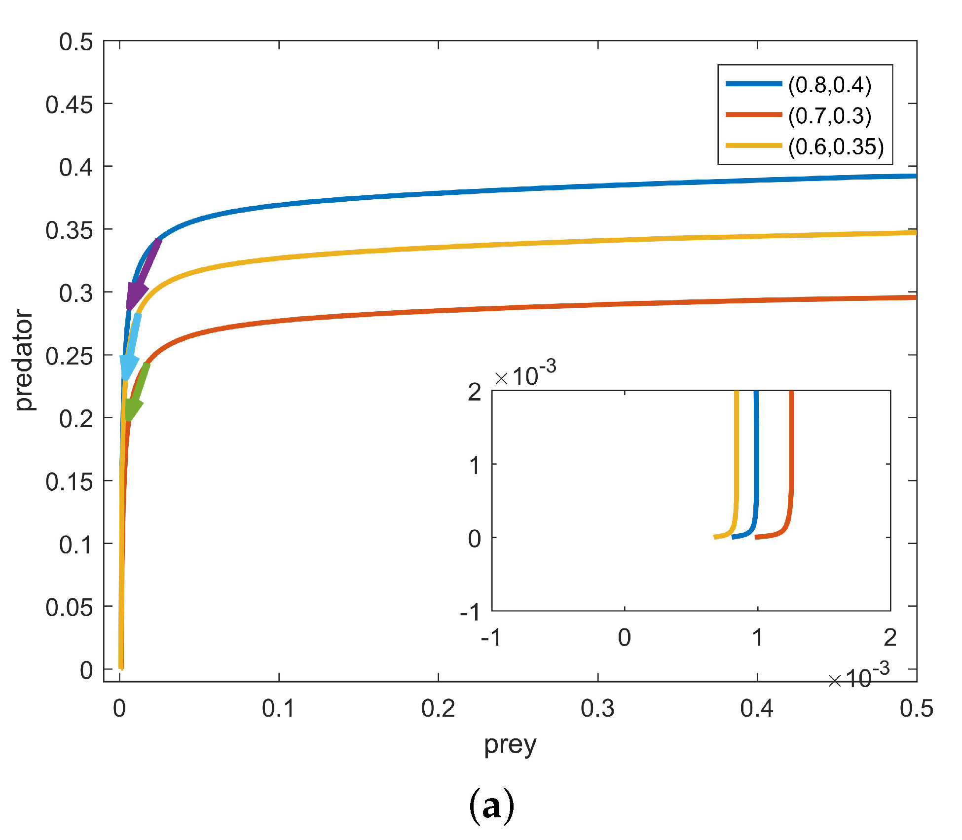
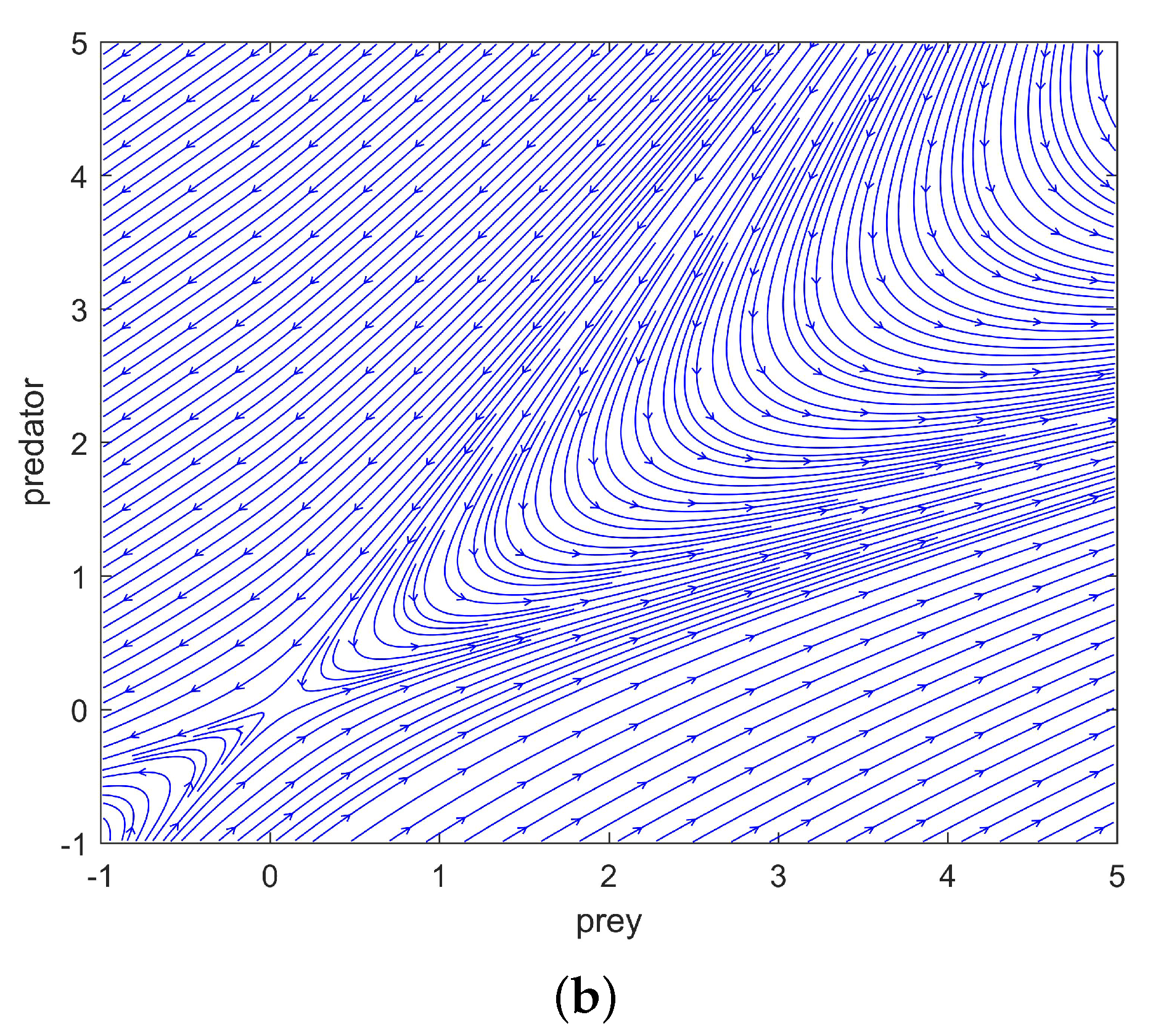
In Figure 1, the parameter values in system (1.3) are $c=0.015$, $k=0.3$, $a=0.1$, $b=0.9$, $d=0.3$, $h=0.2$, $g=0.1$ and $\alpha =0.98$. Figure 1a displays the trajectories of system (1.3) starting from different points. Although it can be observed that system (1.3) exhibits a saddle at the origin, it is not entirely clear. To provide a more clear representation of the behavior of system (1.3) at the origin, we constructed streamline plots, depicted in Figure 1b. From Figure 1b, it is evident that system (1.3) possesses a saddle at the origin.

Figure 1. (a) shows the trajectories of system (1.3) starting from points $(0.8,0.4)$, $(0.7,0.3)$ and $(0.6,0.35)$, respectively; (b) represents the streamline plots of system (1.3) at the origin.

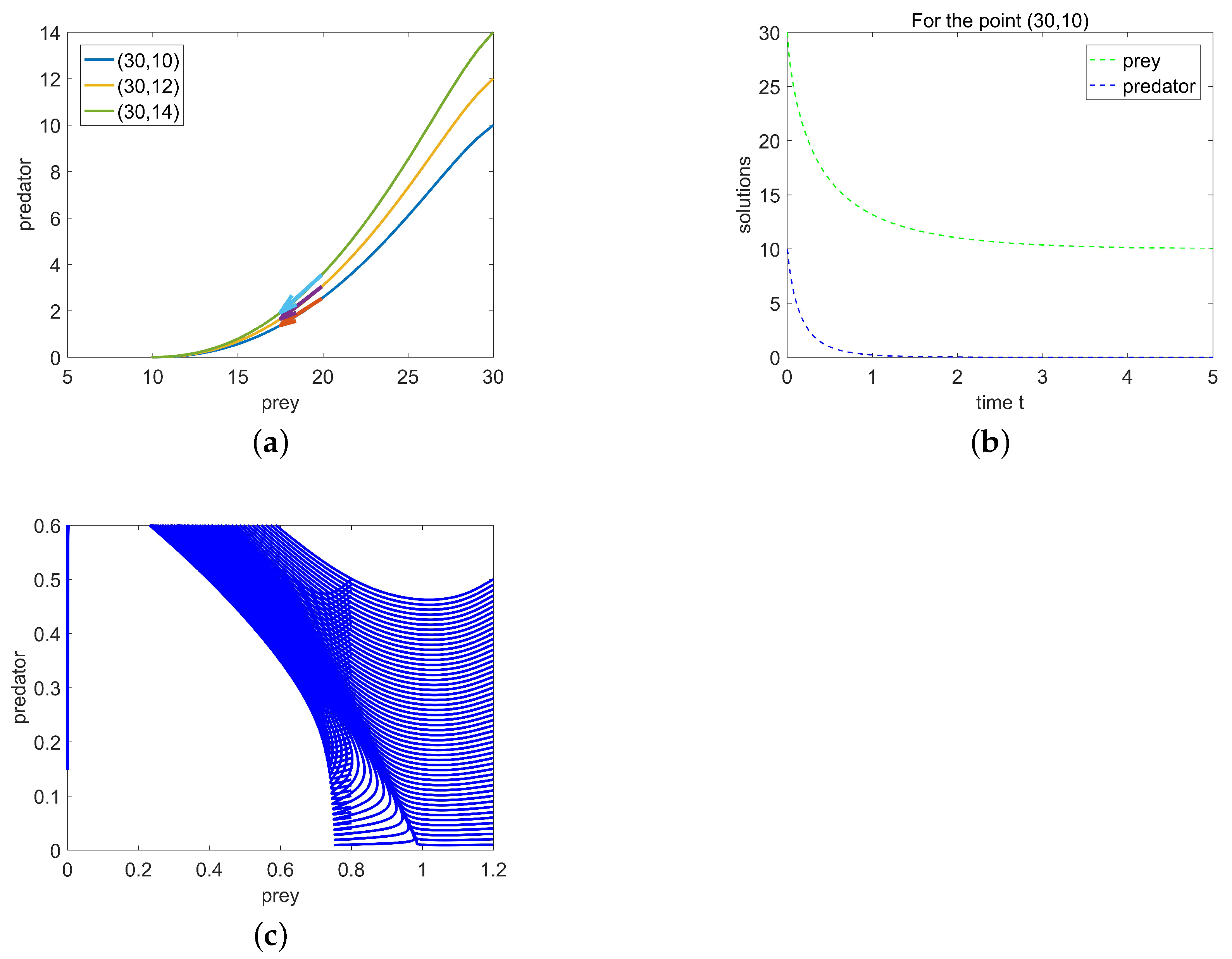
In Figure 2a,b, the parameter values of system (1.3) are $c=0.9$, $k=10$, $b=0.2$, $a=3$, $h=0.9$, $d=0.2$, $g=0.2$ and $\alpha =0.98$, which satisfy $d>\frac{cbk}{h+k^2}-gk$. Figure 2a shows that the behavior of system (1.3), regardless of whether it starts from the point $(30,10)$, $(30,12)$ or $(30,14)$, will eventually converge to the point (10, 0). Figure 2b demonstrates how the populations of prey and predator change over time when starting from the point $(30,10)$. We can observe that as time increases, the population of prey tends to 10, while the predator becomes extinct. In Figure 2c, the parameter values of system (1.3) are $c=0.6$, $k=1$, $b=0.5$, $a=0.1$, $h=0.6$, $d=0.1$, $g=0.1$ and $\alpha =0.98$, which satisfy $d<\frac{cbk}{h+k^2}-gk$. We can clearly see that system (1.3) exhibits a saddle at the boundary equilibrium point $(1,0)$.

Figure 2. (a) The properties of system (1.3) at the boundary equilibrium point (10,0) for $d>\frac{cbk}{h+k^2}-gk$; (b) the quantities of prey and predators starting from the point $(30,10)$ over time; (c) the properties of system (1.3) at the boundary equilibrium point (1,0) for $d<\frac{cbk}{h+k^2}-gk$.

For the positive equilibrium point of system (1.3), we are interested in its bifurcation behavior. In Figure 3, the parameter values of system (1.3) are $c=0.6$, $b=0.5$, $a=0.1$, $h=0.6$, $d=0.1$, $g=0.1$ and $\alpha =0.98$. Figure 3a,b shows that the positive equilibrium point $Q_1(u_1,v_1)$ is stable and unstable when $k=1$ and $k=10$, respectively. Furthermore, we can see from Figure 3b that when k crosses the critical value, a stable limit cycle emerges, indicating the occurrence of a supercritical Hopf bifurcation in system (1.3).

Figure 3. The existence of a supercritical Hopf bifurcation of system (1.3) with the parameter values $c=0.6$, $b=0.5$, $a=0.1$, $h=0.6$, $d=0.1$, $g=0.1$ and $\alpha =0.98$ for $k=1$ (a) and $k=10$ (b).

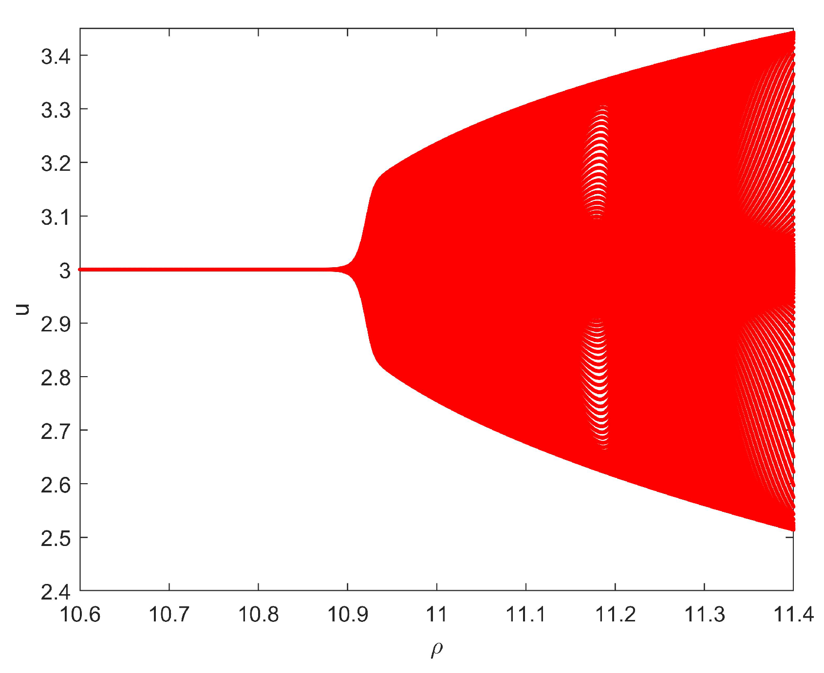
With values of $\alpha =0.75,b=0.9,a=0.2,k=3,h=5,c=0.7,d=0.2$ and $g=0.1$, Figure 4 is the bifurcation diagram of system (1.6) starting from the point $(u_0,v_0)=(0.6,0.1)$, and we can clearly observe that system (1.6) undergoes a period-doubling bifurcation at the critical value. With values of $\alpha =0.75,b=0.9,a=0.2,k=3,h=5,c=1,d=0.2,g=0.1$, Figure 5 is the bifurcation diagram of system (1.6) starting from the point $(u_0,v_0)=(0.5,0.1)$, and it is clear that system (1.6) undergoes a Neimark–Sacker bifurcation at the critical value.

Figure 4. The existence of a period-doubling bifurcation of system (1.6) with the k taking values from 8 to $11.6$.

Figure 5. The existence of a Neimark–Sacker bifurcation of system (1.6) with the k taking values from $10.6$ to $11.4$.

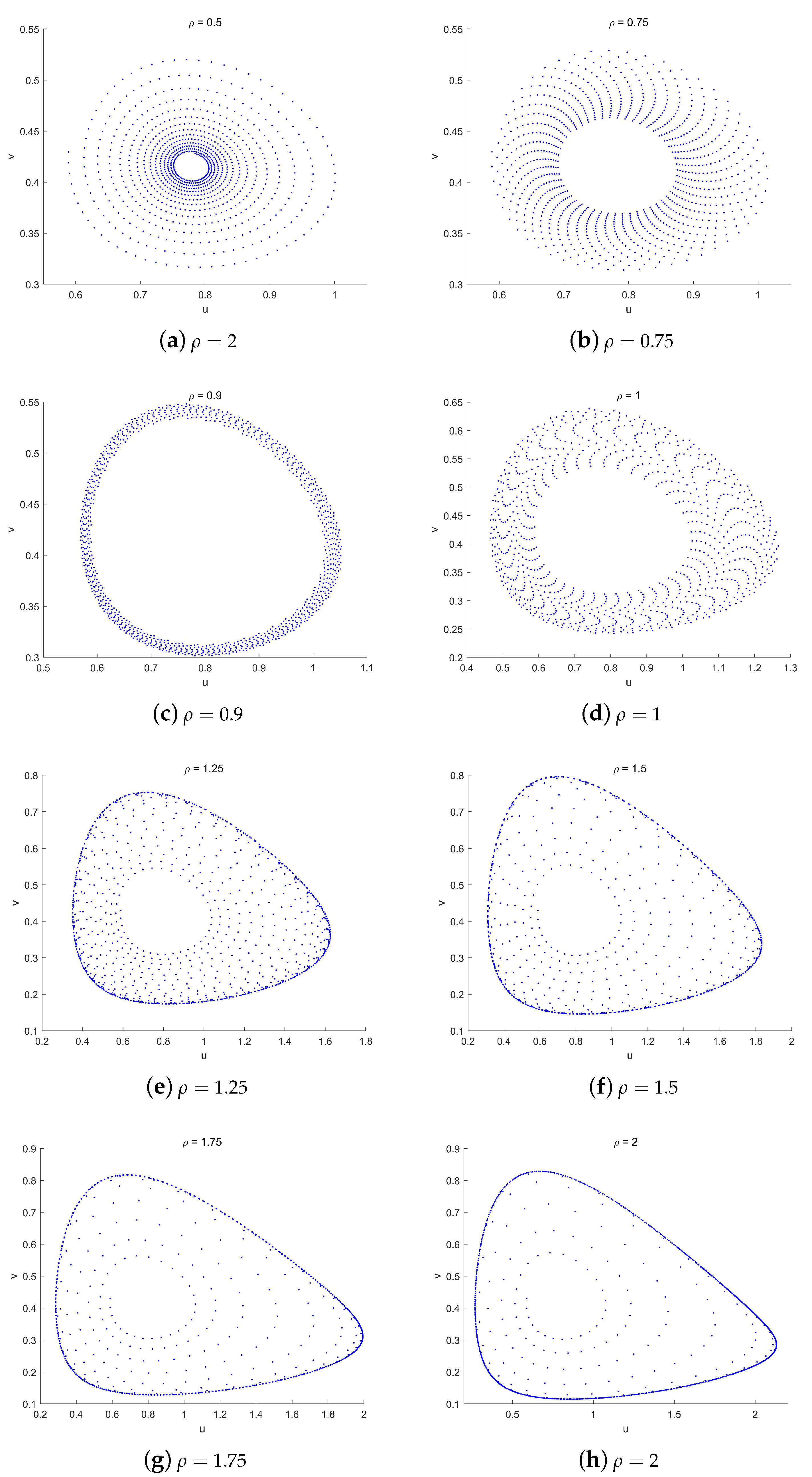
Figure 6 depicts the phase diagram of system (1.6) starting from the point $(u_0,v_0)=(0.5888,4.324)$ with parameters $\alpha =0.75,b=0.9,a=0.2,k=3,h=5,$ $c=1,$ $d=0.2,g=0.1$. We can observe that as $\rho$ increases, the equilibrium point gradually transitions from a stable focus to an unstable focus, and a stable limit cycle emerges.

Figure 6. Phase portraits of system (1.6) with $\alpha =0.75,b=0.9,a=0.2,k=3,h=5,c=1,$ $d=0.2,$ $g=0.1$ and different $\rho$ when the initial value $(x_0,y_0)=(0.5888,0.4324)$.

7. Conclusions

In this paper, we propose a fractional-order predator–prey model with a Holling type IV functional response and anti-predator behavior. According to the discrete and continuous versions, from two different perspectives we analyzed their dynamical behavior in detail, including the feasibility, existence and stability of equilibrium points and the possibility of local bifurcations. Our main aim is to provide readers with a better understanding of the dynamics of the system. As there is currently a lack of effective ways and methods to study the dynamics of fractional-order differential systems, in this paper, we propose an effective way to consider this problem from different angles—both continuous and discrete. This is the novelty of this paper. Indeed, we find that there exist some differences in the dynamics of the system between the continuous version and the discrete version. Numerical simulations also illustrate corresponding theoretical results. By analyzing the dynamical behavior of systems (1.3) and (1.6), respectively, we can deduce the following conclusions:

(1) By analyzing the stability of the equilibrium point $Q_0(0,0)$ and conducting numerical simulations, we can determine that the equilibrium point $Q_0(0,0)$ is a saddle point. This implies that under any conditions existing in nature, the simultaneous extinction of predator and prey does not occur.

(2) Through the study of the dynamical behavior of the boundary equilibrium point $Q_k(k,0)$ and numerical simulations, we have found that when d is large, it leads to the extinction of predator. In this case, the prey population tends towards a stable density. On the other hand, when d is small, the extinction of the predator does not occur, and the prey population tends to a stable state. This indicates that when a detrimental condition for the survival of predator and prey arises in nature, the predator may tend towards extinction, while the prey population, although it may decrease, does not tend towards extinction. Instead, it stabilizes at a certain level.

(3) Based on the analysis and numerical simulations of the positive equilibrium point $Q_1(u_1,v_1)$, we can draw the following conclusions: When the parameter k exceeds a critical value, the system exhibits a stable limit cycle. This implies that the interaction between predator and prey leads to periodic oscillations. The presence of this limit cycle indicates that the system exhibits rich dynamic behavior, and under specific conditions, the populations of predator and prey undergo periodic fluctuations. Therefore, we can achieve a steady coexistence state and eliminate the limit cycle by reducing the environmental carrying capacity to the prey.

(4) Through the bifurcation analysis used in this paper, we find that the analysis methods for bifurcation problems are applicable to other types of fractional differential systems. It is well known that the current analysis methods for bifurcation problems in fractional-order dynamic systems are not well developed. Thus, in order to better understand the dynamics of this system, we discretize the fractional-order system to study its dynamics from a different angle. A richer set of dynamical properties is obtained, indicating that investigations after discretizing this system are indeed more valuable and helpful to understanding the properties of this system.

References

1. Berryman, A.A. The orgins and evolution of predator-prey theory. Ecology 1992, 73, 1530–1535. [Google Scholar] [CrossRef]
2. Wang, W.; Chen, L. A Predator-Prey System with Stage-Structure for Predator. Comput. Math. Appl. 1997, 33, 83–91. [Google Scholar] [CrossRef]
3. Ba, Z.; Li, X. Period-doubling bifurcation and Neimark-Sacker bifurcation of a discrete predator-prey model with Allee effect and cannibalism. Electron. Res. Arch. 2023, 31, 1405–1438. [Google Scholar] [CrossRef]
4. Liu, Y.; Li, X. Dynamics of a discrete predator-prey model with Holling-II functional response. Int. J. Biomath. 2021, 14, 2150068. [Google Scholar] [CrossRef]
5. Qi, H.; Meng, X. Threshold behavior of a stochastic predator–prey system with prey refuge and fear effect. Appl. Math. Lett. 2021, 113, 106846. [Google Scholar] [CrossRef]
6. Blasius, B.; Rudolf, L.; Weithoff, G.; Gaedke, U.; Fussmann, G.F. Long-term cyclic persistence in an experimental predator–prey system. Nature 2020, 577, 226–230. [Google Scholar] [CrossRef]
7. Mukherjee, D. Role of fear in predator–prey system with intraspecific competition. Math. Comput. Simul. 2020, 177, 263–275. [Google Scholar] [CrossRef]
8. Qiu, H.; Guo, S.; Li, S. Stability and Bifurcation in a Predator–Prey System with Prey-Taxis. Int. J. Bifurc. Chaos 2020, 30, 2050022. [Google Scholar] [CrossRef]
9. Perc, M.; Grigolini, P. Collective behavior and evolutionary games–An introduction. Chaos Solitons Fractals 2013, 56, 1–5. [Google Scholar] [CrossRef]
10. Lima, S.L. Stress and Decision Making under the Risk of Predation: Recent Developments from Behavioral, Reproductive, and Ecological Perspectives. Adv. Study Behav. 1998, 27, 215–290. [Google Scholar]
11. Tollrian, R. Predator-Induced Morphological Defenses: Costs, Life History Shifts, and Maternal Effects in Daphnia Pulex. Ecology 1995, 76, 1691–1705. [Google Scholar] [CrossRef]
12. Choh, Y.; Lgnacio, M.; Sabelis, M.W.; Janssen, A. Predator-prey role reversals, juvenile experience and adult antipredator behavior. Lab. Appl. Entomol. 2012, 2, 728. [Google Scholar]
13. Janssen, A.; Faraji, F.; Hammen, T.V.D.; Magalhaes, S.; Sabelis, M.W. Interspecific infanticide deters predators. Ecol. Lett. 2002, 5, 490–494. [Google Scholar] [CrossRef]
14. Saito, Y. Prey kills predator: Counter-attack success of a spider mite against its specific phytoseiid predator. Exp. Appl. Acarol. 1986, 2, 47–62. [Google Scholar] [CrossRef]
15. Ives, A.; Dobson, A. Antipredator behavior and the population dynamics of simple predator-prey systems. Am. Nat. 1987, 130, 431–447. [Google Scholar] [CrossRef]
16. Tang, B.; Xiao, Y. Bifurcation analysis of a predator–prey model with anti-predator behavior. Chaos Solitons Fractals 2015, 70, 58–68. [Google Scholar] [CrossRef]
17. Sokol, W. Oxidation of an Inhibitory Substrate by Washed Celts (Oxidation of Phenol by Pseudornonas putida). Biotechnol. Bioeng. 1987, 30, 921–927. [Google Scholar] [CrossRef]
18. Liouville, J. Troisième mémoire sur le développement des fonctions ou parties de fonctions en séries dont les divers termes sont assujettis à satisfaire à une même équation différentielle du second ordre, contenant un paramètre variable. J. Math. Pures Appl. 1837, 2, 418–436. [Google Scholar]
19. Riesz, M. L’intégrale de Riemann–Liouville et le problème de Cauchy pour l’équation des ondes. Bull. Soc. Math. Fr. 1939, 67, 153–170. [Google Scholar] [CrossRef]
20. Caputo, M. Linear Models of Dissipation whose Q is almost Frequency Independent-II. Geophys. J. R. Astron. Soc. 1976, 13, 529–539. [Google Scholar] [CrossRef]
21. Debnath, S.; Majumdar, P.; Sarkar, S.; Ghosh, U. Memory effect on prey–predator dynamics: Exploring the role of fear effect, additional food and anti-predator behaviour of prey. J. Comput. Sci. 2023, 66, 101929. [Google Scholar] [CrossRef]
22. Singh, A.; Sharma, V.S. Bifurcations and chaos control in a discrete-time prey–predator model with Holling type-II functional response and prey refuge. J. Comput. Appl. Math. 2023, 418, 114666. [Google Scholar] [CrossRef]
23. Kumar, S.; Kumar, R.; Cattani, C.; Samet, B. Chaotic behaviour of fractional predator-prey dynamical system. Chaos Solitons Fractals 2020, 135, 109811. [Google Scholar] [CrossRef]
24. Das, M.; Samanta, G. A delayed fractional order food chain model with fear effect and prey refuge. Math. Comput. Simul. 2020, 178, 218–245. [Google Scholar] [CrossRef]
25. Barman, D.; Roy, J.; Alrabaiah, H.; Panja, P.; Mondal, S.P.; Alam, S. Impact of predator incited fear and prey refuge in a fractional order prey predator model. Chaos Solitons Fractals 2021, 142, 110420. [Google Scholar] [CrossRef]
26. Das, M.; Samanta, G. A prey-predator fractional order model with fear effect and group defense. Int. J. Dyn. Control 2021, 9, 334–349. [Google Scholar] [CrossRef]
27. Yousef, F.; Yousef, A.; Maji, C. Effects of fear in a fractional-order predator-prey system with predator density-dependent prey mortality. Chaos Solitons Fractals 2021, 145, 110711. [Google Scholar] [CrossRef]
28. Zhang, N.; Kao, Y.; Xie, B. Impact of fear effect and prey refuge on a fractional order prey–predator system with Beddington–DeAngelis functional response. Chaos 2022, 32, 043125. [Google Scholar] [CrossRef]
29. Majumdar, P.; Mondal, B.; Debnath, S.; Ghosh, U. Controlling of periodicity and chaos in a three dimensional prey predator model introducing the memory effect. Chaos Solitons Fractals 2022, 164, 112585. [Google Scholar] [CrossRef]
30. Xie, B.; Zhang, Z. Impact of Allee and fear effects in a fractional order prey–predator system incorporating prey refuge. Chaos 2023, 33, 013131. [Google Scholar] [CrossRef]
31. Salmana, S.M.; Yousef, A.M.; Elsadanyc, A.A. Stability, bifurcation analysis and chaos control of a discrete predator-prey system with square root functional response. Chaos Solitons Fractals 2016, 93, 20–31. [Google Scholar] [CrossRef]
32. Yousef, A.M.; Rida, S.Z.; Ali, H.M.; Zaki, A.S. Stability, co-dimension two bifurcations and chaos control of a host-parasitoid model with mutual interference. Chaos Solitons Fractals 2023, 166, 112923. [Google Scholar] [CrossRef]
33. Yousef, A.M.; Rida, S.Z.; Gouda, Y.G.; Zaki, A.S. Dynamical Behaviors of a Fractional-Order Predator–Prey Model with Holling Type IV Functional Response and Its Discretization. Int. J. Nonlinear Sci. Numer. Simul. 2019, 20, 125–136. [Google Scholar] [CrossRef]
34. Singh, A.; Elsadany, A.A.; Elsonbaty, A. Complex dynamics of a discrete fractional-order Leslie-Gower predator-prey model. Math. Methods Appl. Sci. 2019, 42, 3992–4007. [Google Scholar] [CrossRef]
35. Elsonbaty, A.; Elsadany, A.A. On discrete fractional order Lotka Volterra model based on the Caputo diference discrete operator. Math. Sci. 2023, 17, 67–79. [Google Scholar] [CrossRef]
36. Uddin, M.J.; Rana, S.M.S.; Işık, S.; Kangalgil, F. On the qualitative study of a discrete fractional order prey–predator model with the effects of harvesting on predator population. Chaos Solitons Fractals 2023, 175, 113932. [Google Scholar] [CrossRef]
37. Kai, D. The Analysis of Fractional Differential Equations (An Application-Oriented Exposition Using Differential Operators of Caputo Type); Springer Scienc & Business Media: Berlin/Heidelberg, Germany, 2010; Volume 2004, pp. 237–244. [Google Scholar]
38. Li, W.; Li, X.Y. Neimark–Sacker bifurcation of a semi-discrete hematopoiesis model. J. Appl. Anal. Comput. 2018, 8, 1679–1693. [Google Scholar]
39. Cieck, M.; Yakar, C.; Oğur, B. Stability, Boundedness, and Lagrange Stability of Fractional Differential Equations with Initial Time Difference. Sci. World J. 2014, 2014, 939027. [Google Scholar]
40. Odibat, Z.; Shawagfeh, N. Generalized Taylor’s formula. Appl. Math. Comput. 2007, 186, 286–293. [Google Scholar] [CrossRef]
41. Wang, C.; Li, X.Y. Stability and Neimark–Sacker bifurcation of a semi-discrete population model. J. Appl. Anal. Comput. 2014, 4, 419–435. [Google Scholar]
42. Liang, S.; Wu, R.; Chen, L. Laplace transform of fractional order differential equations. Electron. J. Differ. Equ. 2015, 2015, 1–15. [Google Scholar]
43. Kexue, L.; Jigen, P. Laplace transform and fractional differential equations. Appl. Math. Lett. 2011, 24, 2019–2023. [Google Scholar] [CrossRef]
44. Petráš, I. Fractional-Order Nonlinear Systems: Modeling, Analysis and Simulation; Springer: Berlin/Heidelberg, Germany, 2011. [Google Scholar]
45. Deshpande, A.; Daftardar-Gejji, V.; Sukale, Y.V. On Hopf bifurcation in fractional dynamical systems. Chaos Solitons Fractals 2017, 98, 189–198. [Google Scholar] [CrossRef]