Estimation and Testing of Random Effects Semiparametric Regression Model with Separable Space-Time Filters

Abstract

This paper focuses on studying a random effects semiparametric regression model (RESPRM) with separable space-time filters. The model cannot only capture the linearity and nonlinearity existing in a space-time dataset, but also avoid the inefficient estimators caused by ignoring spatial correlation and serial correlation in the error term of a space-time data regression model. Its profile quasi-maximum likelihood estimators (PQMLE) for parameters and nonparametric functions, and a generalized F-test statistic for checking the existence of nonlinear relationships are constructed. The asymptotic properties of estimators and asymptotic distribution of test statistic are derived. Monte Carlo simulations imply that our estimators and test statistic have good finite sample performance. The Indonesian rice farming data are used to illustrate our methods.

1. Introduction

A space-time panel dataset is a sample collected from a number of spatial units over time periods. Such data widely exist in various research fields. It is of great theoretical significance and practical value to conduct statistical modeling and analysis on space-time panel data. There are three branches of panel data which are defined as ordinary panel data, spatial panel data, and space-time panel data given the variety heterogeneities of existing panel datasets. The regression models established on basis of ordinary panel data are called ordinary panel data regression models. Ordinary panel data regression models date back to the 1950s when the pioneering paper (Bates et al. [1]) was published. After that, the theories and methods of ordinary panel data regression models have been greatly enriched and they are widely available in many fields, such as economics, management and environmental science, see Chamberlain [2], Baltagi [3], Arellano [4], Baldev and Baltagi [5], and Hsiao [6], among others. Panel data spatial regression models generated from the turn of this century when spatial econometrics literature has exhibited a particular interest in the specification and estimation of econometric relationships based on spatial panel data (Elhorst [7]). Panel data spatial regression models deal with the spatial correlations between different individual units in panel data models and their theories have been well developed and widely used, see Druska and Horrace [8]; Egger, Pfaffermayr, and Winner [9]; Kapoor, Kelejian, and Prucha [10]; Lee and Yu [11], etc.

Two problems hampering when modeling with space-time panel data are serial correlation and spatial correlation. Serial correlation lies between the observations of each spatial unit over time, and it is the domain of the voluminous time-series econometrics literature. Spatial correlation lies between the observations of the spatial units at each time period, and it is of the spatial econometrics literature, a subfield of econometrics for dealing with spatial interaction effects among geographical units such as individuals, firms, governments, etc. In order to overcome the defects that the panel data spatial regression models do not account for serial correlation and the ordinary panel data regression models account for neither spatial correlation nor serial correlation, people have tried to combine serial correlation and spatial correlations, and established panel data paramertic regression models with separable/nonseparable space-time filters, which are used to do researches on estimation, testing and empirical analysis. Elhorst [12] developed ML method of a panel data linear regression model with nonseparable space-time filters, while did not establish asymptotic properties of the estimators. Parent and LeSage [13] explored Markov Chain Monte Carlo methods of random effects panel data linear regression models with separable space-time filters, and the performance of the method was demonstrated by both Monte Carlo simulations and an applied illustration. Lee and Yu [14] studied MLE and its asymptotic properties of fixed and random effects panel data parametric regression models with separable space-time filters. Lee and Yu [15] provided QMLE and its asymptotic properties for a fixed effects panel data linear regression model with disturbances contained both separable space-time filters and nonseparable space-time filters. Baltagi et al. [16] derived several Lagrange Multiplier tests for panel data linear regression model with separable space-time fliters containing random effects. Cohen and Paul [17] analysed the influencing factors of public infrastructure investment on the costs and productivity of private enterprises on basis of 1982–1996 state-level U.S. manufacturing data by panel data parametric regression model with separable space-time filters.

All literature on panel data regression models with separable/nonseparable space-time filters mentioned above focuses on panel data parametric regression models. Although the theories and applications of these models have been well developed, they are often unrealistic in real situations for the reason that they fail to capture complex structure (e.g., nonlinearity) owing to lacking of flexibility. Moreover, the form of parametric regression models may be misspecified, and estimators based on misspecified models are able to cause inconsistency and even erroneous conclusions. Driven by these reasons, Zhao et al. [18] constructed semiparametric minimum average variance estimation method, and proposed a F-test statistic of partially linear single-index panel regression model with separable space-time filters, then proved the asymptotic properties of estimators and test statistic. Bai, Hu, and You [19] established weighted semiparametric least squares and weighted polynomial spline series estimation method for parametric and nonparametric component, respectively, of panel data partially linear varying-coefficient regression model with separable space-time filters, and then proved their asymptotic normalities.

In this paper, we study estimation and testing of random effects semiparametric regression model (RESPRM) with separable space-time filters. By allowing a nonparametric component in parametric regression model with separable space-time filters, it can simultaneously capture the linear and nonlinear effects of covariates, spatial correlation of error structure, serial correlation of remainder error structure, and individual random effects. To the best of our knowledge, there is no related literature on this model. In this paper, we aim to study its profile quasi-maximum likelihood estimation (PQMLE) and hypothesis test methods, and then conduct systematic studies of the asymptotic properties and small sample performance for estimators and test statistic. Furthermore, we illustrate the proposed estimation and testing methods by using a real dataset.

The remainder of this paper is organized as follows. Section 2 introduces the RESPRM with separable space-time filters, and estimators for the model and test statistic for nonparametric component are constructed. Section 3 mainly provides asymptotic properties of estimators, asymptotic distribution of test statistic and conditional assumptions. Section 4 presents the finite sample performance of estimates and F-test statistic through Monte Carlo simulations. Section 5 illustrates the proposed methods by an application of Indonesian rice farming data. Conclusions are summarized in Section 6. The proofs of some important lemmas and theorems are given in Appendix A.

2. The Model, Estimation, and Testing

2.1. The Model

The RESPRM with separable space-time filters can be specified as:

$$\begin{array}{cc}\hfill y_{it}& =x_{it}^{\prime }\beta +m\left(z_{it}\right)+b_i+{\epsilon }_{it},\hfill \end{array}$$

(1)

$$\begin{array}{cc}\hfill {\epsilon }_{it}& =\rho \sum _{j=1}^N{w}_{ij}{\epsilon }_{jt}+{\nu }_{it},\hfill \end{array}$$

(2)

$$\begin{array}{cc}\hfill {\nu }_{it}& =\lambda {\nu }_{i,t-1}+e_{it},1\le i\le N,1<t\le T,\hfill \end{array}$$

(3)

where $y_{it}$ is an observation of the response variable for the ith spatial unit at the tth time period, $x_{it}={(x_{it1},x_{it2},\dots ,x_{itp})}^{{}^{\prime }}$, and $z_{it}={(z_{it1},z_{it2},\dots ,z_{itq})}^{{}^{\prime }}$ are observations of $p\times 1$ and $q\times 1$ vectors of covariates, respectively, $b_i$ is an individual random effect which is assumed to be $IID(0,{\sigma }_b^2)$, ${\epsilon }_{it}$ is an error term, ${\nu }_{it}$ is a remainder error term which is weakly stationary sequence, $e_{it}$ is a random error term which is assumed to be $IID(0,{\sigma }_e^2)$, $\beta ={({\beta }_1,{\beta }_2,\dots ,{\beta }_p)}^{\prime }$ is a regression coefficient vector of $x_{it}$, $m(·)$ is an unknown link function, $w_{ij}$ is the $(i,j)$th element of spatial weights matrix, $\rho$ and $\lambda$ are spatial correlation and series correlation coefficients, respectively. Furthermore, we denote ${\theta }_0={({\zeta }_0^{\prime },{\beta }_0^{\prime })}^{\prime }$, ${\zeta }_0=({\rho }_0,{\lambda }_0,{\sigma }_{b0}^2,{\sigma }_{e0}^2)$ as the true parameter vector of $\theta ={({\zeta }^{\prime },{\beta }^{\prime })}^{\prime }$ and $\zeta =(\rho ,\lambda ,{\sigma }_b^2,{\sigma }_e^2)$, respectively, and $m_0\left(z\right)$ as the true value of nonparametric function of $m\left(z\right)$.

We find that separable space-time filters in our model result in a trade-off between the spatial correlation and serial correlation coefficients. According to Shi and Lee [20], it is not hard to obtain that the stationarity requires not only $\left|\rho \right|<1,\left|\lambda \right|<1$, but also $\left|\lambda \right|+\left|\rho \right|+\left|\rho \lambda \right|<1$, i.e., parameter space $\Lambda$ of $\lambda$ and $\rho$, see Figure 1.

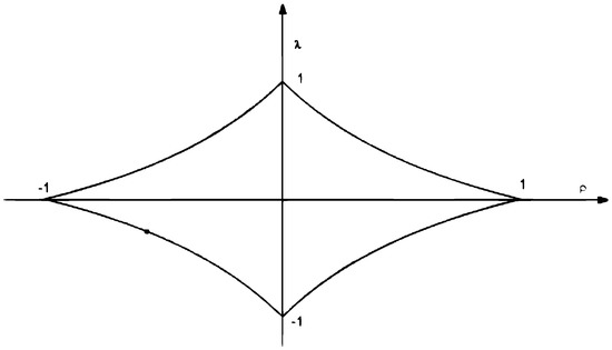
Figure 1. The parameter space $\Lambda$ of $\lambda$ and $\rho$.

2.2. Estimation

Because that random effect $b_i$ could be regarded as time-invariant permanent spillovers (see Baltagi, Fingleton, and Pirotte [21]), the model (1) can be written in matrix form

$$Y=X\beta +M+\eta ,$$

(4)

where $Y={(y_{11},\dots ,y_{NT})}^{\prime }$, $X={(x_{11},\dots ,x_{NT})}^{\prime }$, $M={(m\left(z_{11}\right),\dots ,m\left(z_{NT}\right))}^{\prime }$, $b={(b_1,\dots ,b_N)}^{\prime }$, $\nu ={({\nu }_{11},\dots ,{\nu }_{NT})}^{\prime }$, $\eta =l_T\otimes b+(I_T\otimes B^{-1})\nu$, $l_T$ is a $T\times 1$ vector of ones, $B=I_N-\rho W$, $I_N$ is an $N\times N$ identity matrix, W is an $N\times N$ spatial weights matrix. Then we obtain the variance matrix of transformed error structure $\eta$ as follows

$$\mathsf{\Omega }=E\left(\eta {\eta }^{\prime }\right)={\sigma }_b^2(l_T{l}_T^{\prime }\otimes I_N)+{\sigma }_e^2[V_{\lambda }\otimes \left(B^{-1}{B}^{-1^{\prime }}\right)],$$

$${\mathsf{\Omega }}^{-1}=\frac{1}{d^2(1-{\lambda }^2)}{V}_{\lambda }^{-1}{l}_T{l}_T^{\prime }{V}_{\lambda }^{-1}\otimes Z_0+[V_{\lambda }^{-1}-\frac{1}{d^2(1-{\lambda }^2)}{V}_{\lambda }^{-1}{l}_T{l}_T^{\prime }{V}_{\lambda }^{-1}]\otimes \left(\frac{1}{{\sigma }_b^2}B{B}^{\prime }\right),$$

$$\left|\mathsf{\Omega }\right|=|V_{\lambda }{|}^N|{\sigma }_e^2{B}^{-1}{B}^{{}^{\prime }-1}{|}^{T-1}\left|Z_0^{-1}\right|,$$

where

$$V_{\lambda }=\frac{1}{1-{\lambda }^2}\left(\begin{array}{cccc}1& \lambda & \dots & {\lambda }^{T-1}\\ \lambda & 1& \dots & {\lambda }^{T-2}\\ ⋮& ⋮& \ddots & ⋮\\ {\lambda }^{T-1}& {\lambda }^{T-2}& \dots & 1\end{array}\right),$$

$Z_0={[d^2(1-{\lambda }^2){\sigma }_b^2{I}_N+{\sigma }_e^2{B}^{-1}{B}^{{}^{\prime }-1}]}^{-1}$, $d^2=l_T^{{}^{\prime }\lambda }{l}_T^{\lambda }=\frac{1+\lambda }{1-\lambda }+(T-1)$ and $l_T^{\lambda }$ = ${(\frac{\sqrt{1+\lambda }}{\sqrt{1-\lambda }},1,\dots ,1)}^{\prime }$. Therefore, the log-likelihood function of the new transformed model (4) is defined in (5)

$$\begin{array}{cc}\hfill lnL\left(\theta \right)& =-\frac{NT}{2}ln\left(2\pi \right)-\frac{1}{2}ln\left|\mathsf{\Omega }\right|-\frac{1}{2}{\xi }^{\prime }\left(\theta \right){\mathsf{\Omega }}^{-1}\xi \left(\theta \right),\hfill \end{array}$$

(5)

where $\xi \left(\theta \right)=Y-M-X\beta$.

It is difficult to obtain the QMLE by maximizing (5) because that $M^{*}$ is unknown. Thus, we will combine PQML method and Working Independence theory (Cai [22]) to estimate unknown parameters and nonparametric function of the model. Working independence assumption is often used to deal with nonparametric/semiparametric regression models which exist correlation structures. By ignoring the correlation structure entirely, and pretending as if the data within a cluster were independent, the asymptotically most efficient estimator of nonparametric function is obtained (Lin and Carroll [23]). It has been widely used in various correlation structures of nonparametric/semiparametric models, such as Fan et al. [24], Fan and Zhang [25], and Tang and Liu [26], among others.

The estimation steps are as follows:

Step 1. By supposing that $\beta$ is known, the initial estimator of $m\left(z\right)$ can be obtained. Let

$$K_H\left(z\right)=diag(k_H(z_{11}-z),\dots ,k_H(z_{1T}-z),\dots ,k_H(z_{N1}-z),\dots ,k_H(z_{NT}-z)),$$

$$\overrightarrow{Z}\left(z\right)={(Z_{11}\left(z\right),\dots ,Z_{1T}\left(z\right),\dots ,Z_{N1}\left(z\right),\dots ,Z_{NT}\left(z\right))}^{\prime },$$

where $k_H\left(z\right)={\left|H\right|}^{-1}k\left(H^{-1}z\right)$, $k(·)$ is $q\times 1$ kernel function, $\left|H\right|$ is the determinant of $H=diag(h_1,\dots ,h_q)$, $Z_{it}\left(z\right)={[1,{H^{-1}(z_{it}-z)}^{\prime }]}^{\prime }$. In addition, denote ${\widehat{m}}_{IN}\left(z\right)={\widehat{a}}_1$, then we have $\widehat{\delta }={({\widehat{a}}_1,{\left(H{\widehat{a}}_2\right)}^{\prime })}^{\prime }$ and

$$\widehat{\delta }=\underset{a_1,a_2}{argmin}\frac{1}{NT}{[\tilde{Y}-\overrightarrow{Z}\left(z\right)\delta ]}^{\prime }{K}_H\left(z\right)[\tilde{Y}-\overrightarrow{Z}\left(z\right)\delta ],$$

where $\tilde{Y}={({\tilde{y}}_{11},\dots ,{\tilde{y}}_{1T},\dots ,{\tilde{y}}_{N1},\dots ,{\tilde{y}}_{NT})}^{\prime }$, ${\tilde{y}}_{it}=y_{it}-x_{it}^{\prime }\beta$, $a_2$ is the first derivative of $m\left(z\right)$. Let $S\left(z\right)={\left[{\overrightarrow{Z}}^{\prime }\left(z\right)K_H\left(z\right)\overrightarrow{Z}\left(z\right)\right]}^{-1}{\overrightarrow{Z}}^{\prime }\left(z\right)K_H\left(z\right)$, then $\widehat{\delta }=S\left(z\right)\tilde{Y}$ and

$${\widehat{m}}_{IN}\left(z\right)=s^{\prime }\left(z\right)\tilde{Y},$$

(6)

where $s\left(z\right)=e_0^{\prime }S\left(z\right)$, $e_0={(1,0,\dots ,0)}^{\prime }$ is a $(q+1)\times 1$ vector.

Step 2. Substituting (6) into (5), the approximate log-likelihood function is given by

$$\begin{array}{cc}\hfill lnL(\theta ,{\widehat{m}}_{IN}\left(z\right))& =-\frac{NT}{2}ln\left(2\pi \right)-\frac{1}{2}ln\left|\mathsf{\Omega }\right|-\frac{1}{2}{(Y-X\beta )}^{\prime }{(I-S)}^{\prime }{\mathsf{\Omega }}^{-1}(I-S)(Y-X\beta ).\hfill \end{array}$$

(7)

By maximizing (7), the initial estimators of $\beta$ can be obtained as follows

$$\begin{array}{c}\hfill {\widehat{\beta }}_{IN}={\left[X^{\prime }{(I-S)}^{\prime }{\mathsf{\Omega }}^{-1}(I-S)X\right]}^{-1}{X}^{\prime }{(I-S)}^{\prime }{\mathsf{\Omega }}^{-1}(I-S)Y,\end{array}$$

(8)

Step 3. Substituting ${\widehat{\beta }}_{IN}$ into (7), we get the concentrated log-likelihood function of $\rho$ and $\lambda$ as

$$\widehat{\zeta }=\underset{\zeta }{argmax}lnL\left(\zeta \right).$$

(9)

Step 4. Substituting (9) into (8), the ultimate estimator of $\widehat{\beta }$ is obtained, and further substituting $\widehat{\beta }$ into (6), the ultimate estimator of $\widehat{m}\left(z\right)$ is obtained.

2.3. Testing

By allowing nonparametric component in a parametric regression model with separable space-time filters, it provides us the ability to explore potential nonlinear relationship lies between covariates and response variable. In order to check whether the parametric specification is correct, it is necessary to do the following hypothesis test

$$H_0:m\left(z_{it}\right)={\gamma }_0+\sum _{j=1}^q{\gamma }_j{z}_{itj}\leftrightarrow H_1:m\left(z_{it}\right)\ne {\gamma }_0+\sum _{j=1}^q{\gamma }_j{z}_{itj},$$

where ${\gamma }_0\dots ,{\gamma }_q$ are unknown parameters. Following Fan, Zhang, and Zhang [27], we obtain $\widehat{m}\left(z_{it}\right)$ by PQML method, and $\tilde{m}\left(z_{it}\right)={\tilde{\gamma }}_0+{\sum }_{j=1}^q{\tilde{\gamma }}_j{z}_{itj}$ is OLS estimator of the intercept and slopes in the linear regression of $y_{it}-x_{it}^{\prime }\widehat{\beta }$, $\widehat{\beta }$ is also obtained by PQML method. The resulting residual sums of squares under the null and alternative hypotheses, respectively, are as follows

$$\begin{array}{c}\hfill RSS\left(H_0\right)=\sum _i^N\sum _{t=1}^T{[y_{it}-\tilde{m}\left(z_{it}\right)-x_{it}^{\prime }\widehat{\beta }]}^2,\\ \hfill RSS\left(H_1\right)=\sum _i^N\sum _{t=1}^T{[y_{it}-\widehat{m}\left(z_{it}\right)-x_{it}^{\prime }\widehat{\beta }]}^2.\end{array}$$

To test the null hypothesis, we define generalized F-test statistic as follows:

$$F_{NT}=\frac{NT}{2}\frac{RSS\left(H_0\right)-RSS\left(H_1\right)}{RSS\left(H_1\right)}.$$

(10)

The asymptotic distribution of $F_{NT}$ is given in Section 3.

3. Asymptotic Property

To prove the asymptotic properties of PQMLE and asymptotic distribution of generalized F-test statistic proposed in Section 2, we need to establish some useful assumptions and lemmas.

3.1. Assumptions

In order to provide a rigorous theoretical analysis, we make the following assumptions.

Assumption 1.

(i)${\{x_i,z_i\}}_{i=1,t=1}^{N,T}$ are nonstochastic variables and uniformly bounded (UB) in $\mathcal{X}\times \mathcal{Z}$.

(ii) 

There is a positive density function $f_t(·)$ such that $\underset{N\to \infty }{lim}\frac{1}{N}{\sum }_{i=1}^N\upsilon \left(z_i\right)=\int \upsilon \left(z\right)f_t\left(z\right)dz$ for any bounded continuous function $\upsilon (·)$, and $f_t(·)$ is bounded away from zero on $\mathcal{Z}$.

(iii) 

$e_{it}$ are iid and $E\left(\right|e_{it}{|}^4)<\infty$.

Assumption 2.

(i)W is a row normalized and prespecified spatial weights matrix.

(ii) 

B is nonsingular.

(iii) 

B and $B^{-1}$ are UB in both row and column sums in absolute value.

Assumption 3.

As $N\to \infty$, $\parallel H\parallel \to 0$, ${N\left|H\right|}^2\to \infty$, ${\parallel H\parallel }^4{\left|H\right|}^{-1}\to 0$ and ${N\left|H\right|\parallel H\parallel }^4\to c\in [0,\infty )$, where $\parallel H\parallel ={tr\left(H^{\prime }H\right)}^{\frac{1}{2}}=\{{\sum }_{ij}|h_{ij}{{|}^2\}}^{\frac{1}{2}}$ is the Euclidean norm of matrix H, and $\left|H\right|$ is the determinant of matrix H.

Assumption 4.

The kernel function $K(·)$ is a continuous density with compact support on $R^q$, all odd order moments of K vanish. Further, $K(·)$ is bounded, $u^{3}K\left(u\right)$ and $u^3{K}^{\prime }\left(u\right)$ are bounded and $\int u^{4}K\left(u\right)du<\infty$.

Assumption 5.

For any $(\rho ,\lambda )\in \mathsf{\Lambda }$, we require that

$$\underset{N,T\to \infty }{lim}[\frac{1}{NT}ln|{\mathsf{\Omega }}_0|+1-\frac{1}{NT}ln\left|\mathsf{\Omega }\right|-tr\left({\mathsf{\Omega }}^{-1}{\mathsf{\Omega }}_0\right)]\ne 0,$$

where

$$|{\mathsf{\Omega }}_0|=|V_{{\lambda }_0}{|}^N|{\sigma }_{e0}^2{B}_0^{-1}{B}_0^{{}^{\prime }-1}{|}^{T-1}\left|Z_{00}^{-1}\right|.$$

$$V_{{\lambda }_0}=\frac{1}{1-{\lambda }_0^2}\left(\begin{array}{cccc}1& {\lambda }_0& \dots & {\lambda }_0^{T-1}\\ {\lambda }_0& 1& \dots & {\lambda }_0^{T-2}\\ ⋮& ⋮& \ddots & ⋮\\ {\lambda }_0^{T-1}& {\lambda }_0^{T-2}& \dots & 1\end{array}\right),$$

$Z_{00}={[d^2(1-{\lambda }_0^2){\sigma }_{b0}^2{I}_N+{\sigma }_{e0}^2{B}^{-1}{B}_0^{{}^{\prime }-1}]}^{-1}$, $d_0^2=l_T^{{}^{\prime }{\lambda }_0}{l}_T^{{\lambda }_0}=\frac{1+{\lambda }_0}{1-{\lambda }_0}+(T-1)$ and

$l_T^{{\lambda }_0}={(\frac{\sqrt{1+{\lambda }_0}}{\sqrt{1-{\lambda }_0}},1,\dots ,1)}^{\prime }$.

Assumption 6.

$L_{11}(L_{44}{L}_{22}-L_{24}^2)-L_{14}(L_{14}{L}_{22}+2L_{12}{L}_{24})>0,$ where $L_{11}=\frac{2tr\left[{\left(B^{-1}\left({\rho }_0\right)W\right)}^2\right]}{N}$, $L_{44}=\frac{1}{2{\sigma }_{e0}^4}$, $L_{22}=-\frac{tr\left({\ddot{C}}_0{C}_0^{-1}\right)+tr\left(C_0^{-1^{\prime }}{\dot{C}}_0^{\prime }\dot{C_0}{C}_0^{-1}\right)}{T}+\frac{1-3{\lambda }_0^2}{T(1-{\lambda }_0^2)}$, $L_{14}=\frac{tr\left(W{B}_0^{-1}\right)}{N{\sigma }_{e0}^2}$, $L_{24}=\frac{tr\left(C_0^{-1^{\prime }}{\dot{C}}_0^{\prime }\right)}{T{\sigma }_{e0}^2}$, $L_{12}=-\frac{2}{NT}tr(C_0^{-1^{\prime }}\dot{C}\otimes W{B}_0^{-1})$.

Remark: Assumption 1 concerns the features of covariates, random error term, and density function for the model (1). Assumption 2 provides the basic features of spatial weight matrix, it parallels Assumption 3 of Su and Jin [28] and Assumption 5 of Lee [29]. The assumption that B and $B^{-1}$ are UB limits the spatial correlation to a manageable degree. Assumption 3 concerns the bandwidth sequence, it parallels Assumption 4 of Hamilton and Truong [30], and Assumption 7 of Ullah and Su [31]. Assumption 4 concerns the kernel function. Assumptions 5 and 6 are necessary for the consistency and asymptotic properties of the estimators.

3.2. Asymptotic Properties

From the model (4), we obtain the reduced form equation of Y as

$$Y=X{\beta }_0+M_0+{\eta }_0.$$

(11)

Let $S=(s_{11},\dots ,s_{NT})$, where $s_{it}=s\left(z_{it}\right)$. Denote a typical entry of $s\left(z\right)$ by

$s(z_{it},z)=e^{\prime }{\left[{\overrightarrow{Z}}^{\prime }\left(z\right)K_H\left(z\right)\overrightarrow{Z}\left(z\right)\right]}^{-1}{\overrightarrow{Z}}_{it}^{\prime }\left(z\right)K_H(z_{it}-z)$, where ${\overrightarrow{Z}}_{it}^{\prime }\left(z\right)$ is a typical column of ${\overrightarrow{Z}}^{\prime }\left(z\right)$.

Lemma 1.

Suppose that Assumptions 1–5 hold, then we have

$$\parallel S\parallel =O_p(N^{-1/2}{\left|H\right|}^{-1/2}).$$

The proof is given by Hamilton and Truong [30].

Lemma 2.

Suppose that Assumptions 1–5 hold, then we have

(i) 

$s(z_{it},z)=N^{-1}{K}_H(z_{it}-z)\overline{f}\left(z\right)\{1+o_p\left(1\right)\}$, where $\overline{f}\left(z\right)={\sum }_{t=1}^T{f}_t\left(z\right)$.

(ii) 

There is a positive constant c such that $\underset{N\to \infty }{lim}P\{N^{-1}{\left[{\overrightarrow{Z}}^{\prime }\left(z\right)K_H\left(z\right)\overrightarrow{Z}\left(z\right)\right]}_{ij}\le c$ for $z\in c_f,i,j=1,\dots ,q+1\}=1$.

(iii) 

There exists a positive constant c such that

$$\underset{N\to \infty }{lim}P\{\underset{z}{sup}\underset{1\le i\le N,1\le t\le T}{max}|s(z_{it},z)|\le c{\left(NT\right)}^{-1}{\left|H\right|}^{-1}\}=1.$$

The proofs is given by Ullah and Su [31].

Lemma 3.

Suppose that Assumptions 1–5 hold, then we have

$$\parallel (I-S)M\parallel =Op(\parallel H{\parallel }^2).$$

The proof is given by Hamilton and Truong [30].

With the above lemmas, we then state main results as follows. Their detail proofs can be found in the Appendix A.

Theorem 1.

Suppose that Assumptions 1–5 hold, then we have $\widehat{\theta }-{\theta }_0=o_p\left(1\right)$.

Theorem 2.

Suppose that Assumptions 1–6 hold, then we have

$$\sqrt{NT}(\widehat{\theta }-{\theta }_0)\stackrel{D}{⟶}N(0,{\Sigma }_{{\theta }_0}^{-1}+{\Sigma }_{{\theta }_0}^{-1}{\mathsf{\Omega }}_{\theta }{\Sigma }_{{\theta }_0}^{-1}),$$

where “$\stackrel{D}{⟶}$” means convergence in distribution, ${\Sigma }_{{\theta }_0}=-E\left[\frac{1}{NT}\frac{{\partial }^{2}lnL\left({\theta }_0\right)}{\partial \theta \partial {\theta }^{\prime }}\right]$ is the average Hessian matrix (information matrix when e and b obey normal distributions), ${\mathsf{\Omega }}_{\theta }=E\left({\mathsf{\Omega }}_{{\theta }_{NT}}\right)$ and ${\mathsf{\Omega }}_{{\theta }_{NT}}=\frac{1}{\sqrt{NT}}\frac{\partial lnL\left({\theta }_0\right)}{\partial \theta }·\frac{1}{\sqrt{NT}}\frac{\partial lnL\left({\theta }_0\right)}{\partial {\theta }^{\prime }}+\frac{1}{NT}\frac{{\partial }^{2}lnL\left({\theta }_0\right)}{\partial \theta \partial {\theta }^{\prime }}$.

Theorem 3.

Suppose that Assumptions 1–4 hold, then we have

$$\sqrt{N\left|H\right|}\left(\widehat{\delta }-\delta -Q^{-1}\left(\begin{array}{c}\frac{\overline{f}\left(z\right)}{2}(\int u{u}^{\prime }K\left(u\right)duH\ddot{m}\left(z\right)H)\\ 0\end{array}\right)\right)\stackrel{D}{⟶}N(0,{\sigma }^2\left(\delta \right)),$$

where $\ddot{m}\left(z\right)$ is the second derivative of $m\left(z\right)$, ${\sigma }^2\left(\delta \right)={\sigma }_e^2\{S\left(z\right)D_I{(C_0^{\prime }{C}_0\otimes B_0^{\prime }{B}_0)}^{-1}{D}_I^{\prime }S{\left(z\right)}^{\prime }$, $D_I=I-D_{\widehat{\tilde{\mathbb{U}}}}^{-1}\widehat{\tilde{\mathbb{U}}}(\widehat{C}\otimes {\widehat{B}}^{\prime }\widehat{B})(I-S)$ and $D_{\widehat{\tilde{\mathbb{U}}}}={\widehat{\tilde{\mathbb{U}}}}^{\prime }(I_T\otimes {\widehat{B}}^{\prime }\widehat{B})\widehat{\tilde{\mathbb{U}}}$, $Q=\overline{f}\left(z\right)\left(\begin{array}{cc}1& 0^{\prime }\\ 0& \int u{u}^{\prime }K\left(u\right)du\end{array}\right)$, $\overline{f}\left(z\right)={\sum }_{t=1}^T{f}_t\left(z\right)$.

Theorem 4.

Suppose that Assumptions 1–4 hold, then we have

$$r_k{F}_{NT}\stackrel{D}{⟶}{\chi }_{df}^2,$$

where $r_k=\frac{K\left(0\right)-\frac{1}{2}\int K^2\left(z\right)du}{\int {(K\left(z\right)-\frac{1}{2}K\ast K\left(z\right))}^{2}du}$, $c_k=K\left(0\right)-\frac{1}{2}\int K^2\left(z\right)du$, $K\left(z\right)=diag(H^{-1}k\left(H^{-1}(z_{11}-z)\right),\dots ,H^{-1}k\left(H^{-1}(z_{NT}-z)\right))$, $df=r_k{c}_k\left|\mathcal{Z}\right|/\left|H\right|$, $\mathcal{Z}$ is the support of $z_{it}$ and H is a bandwidth sequence, besides, note that when $K\left(0\right)=maxK\left(z\right)$, we get ${K\left(0\right)>\parallel K\parallel }_2^2$, $c_k>\frac{1}{2}K\left(0\right)$ and hence $r_k>0$.

4. Monte Carlo Simulation

4.1. Performance of the Estimates

In this section, we report the results of a small-scale Monte Carlo study which is aimed to evaluate the finite sample performance of PQMLEs. We use mean square error ($MSE$), standard deviation ($SD$), and mean absolute deviation error ($MADE$) to measure the parametric and nonparametric estimation performance, respectively, where

$${\mathrm{MADE}}_j=Q^{-1}\sum _{q=1}^Q|\widehat{m}\left(z_q\right)-m\left(z_q\right)|,j=1,2,\dots ,mcn,$$

$mcn=2000$, ${\left\{z_q\right\}}_{q=1}^Q$ are Q fixed grid points in support set of z. Furthermore, we apply the rule of thumb method of Mack and Silverman [32] to choose the optimal width and let $K\left(u\right)=\left(\frac{3}{4\sqrt{5}}\right)(1-\frac{1}{5}{u}^2)1(u^2\le 5)$ (see Su [33]).

We use data generated from the following model

$$\begin{array}{cc}\hfill y_{it}& =x_{it}\beta +m\left(z_{it}\right)+b_i+{\epsilon }_{it},\hfill \\ \hfill {\epsilon }_{it}& =\rho \sum _{j=1}^N{w}_{ij}{\epsilon }_{jt}+{\nu }_{it},\hfill \\ \hfill {\nu }_{it}& =\lambda {\nu }_{i,t-1}+e_{it},\hfill \end{array}$$

(12)

where $x_{it}\sim U[-2,2]$, $z_{it}\sim U[-3,3]$, $e_{it}\sim i.i.d.N(0,1)$, $b_i\sim i.i.d.N(0,1)$, $m\left(z_{it}\right)=0.3z_{it}^2$, $\beta =1$, $\rho =0.2$, $0.4$, and $\lambda =0.2$, $0.4$ respectively. In addition, we defined weights matrix as Rook matrix (see Anselin [34]). The simulation results of cases $N=50,100,200$, and $T=10,20$ are presented in Table 1, Table 2, Table 3 and Table 4.

Table 1. Results of parametric estimates under the model (12) with T = 10.

		N = 50			N = 100			N = 200
		True	Mean	MSE	True	Mean	MSE	True	Mean	MSE
	$\widehat{\beta }$	1.0000	0.9854	0.0070	1.0000	1.0096	0.0032	1.0000	1.0060	0.0018
	$\widehat{\rho }$	0.2000	0.2034	0.0108	0.2000	0.2027	0.0089	0.2000	0.2017	0.0044
$\rho =0.2$	$\widehat{\lambda }$	0.2000	0.2079	0.0036	0.2000	0.2074	0.0032	0.2000	0.2027	0.0027
$\lambda =0.2$	$\widehat{{\sigma }_e^2}$	1.0000	1.0335	0.0013	1.0000	1.0245	0.0011	1.0000	1.0064	0.0008
	$\widehat{{\sigma }_b^2}$	1.0000	1.0356	0.0045	1.0000	1.0297	0.0025	1.0000	1.0160	0.0013
	$\widehat{\beta }$	1.0000	1.0130	0.0049	1.0000	1.0041	0.0041	1.0000	1.0004	0.0010
	$\widehat{\rho }$	0.2000	0.2059	0.0113	0.2000	0.2018	0.0103	0.2000	0.2041	0.0010
$\rho =0.2$	$\widehat{\lambda }$	0.4000	0.4120	0.0056	0.4000	0.4046	0.0038	0.4000	0.4039	0.0013
$\lambda =0.4$	$\widehat{{\sigma }_e^2}$	1.0000	1.0567	0.0088	1.0000	1.0302	0.0045	1.0000	1.0290	0.0043
	$\widehat{{\sigma }_b^2}$	1.0000	1.0536	0.0057	1.0000	1.0145	0.0033	1.0000	1.0022	0.0025
	$\widehat{\beta }$	1.0000	1.0349	0.0782	1.0000	1.0311	0.0601	1.0000	0.9774	0.0506
	$\widehat{\rho }$	0.4000	0.3846	0.0344	0.4000	0.4026	0.0409	0.4000	0.3929	0.0311
$\rho =0.4$	$\widehat{\lambda }$	0.2000	0.2069	0.0018	0.2000	0.2055	0.0015	0.2000	0.2044	0.0013
$\lambda =0.2$	$\widehat{{\sigma }_e^2}$	1.0000	1.0429	0.0027	1.0000	1.0159	0.0023	1.0000	1.0083	0.0017
	$\widehat{{\sigma }_b^2}$	1.0000	1.0378	0.0025	1.0000	1.0083	0.0018	1.0000	1.0055	0.0013
	$\widehat{\beta }$	1.0000	1.0356	0.0637	1.0000	1.0116	0.0441	1.0000	1.0071	0.0063
	$\widehat{\rho }$	0.4000	0.4083	0.0011	0.4000	0.4014	0.0010	0.4000	0.4008	0.0005
$\rho =0.4$	$\widehat{\lambda }$	0.4000	0.4109	0.0008	0.4000	0.4107	0.0008	0.4000	0.4009	0.0006
$\lambda =0.4$	$\widehat{{\sigma }_e^2}$	1.0000	1.0411	0.0019	1.0000	1.0212	0.0005	1.0000	1.0041	0.0004
	$\widehat{{\sigma }_b^2}$	1.0000	1.0399	0.0021	1.0000	1.0138	0.0020	1.0000	1.0022	0.0008

Table 2. Results of parametric estimates under the model (12) with T = 20.

		N = 50			N = 100			N = 200
		True	Mean	MSE	True	Mean	MSE	True	Mean	MSE
	$\widehat{\beta }$	1.0000	1.0068	0.0061	1.0000	0.9932	0.0025	1.0000	0.9945	0.0010
	$\widehat{\rho }$	0.2000	0.1976	0.0012	0.2000	0.1990	0.0010	0.2000	0.2003	0.0005
$\lambda =0.2$	$\widehat{\lambda }$	0.2000	0.2051	0.0022	0.2000	0.2019	0.0015	0.2000	0.2008	0.0008
$\rho =0.2$	$\widehat{{\sigma }_e^2}$	1.0000	1.0102	0.0009	1.0000	1.0098	0.0007	1.0000	1.0005	0.0005
	$\widehat{{\sigma }_b^2}$	1.0000	1.0242	0.0034	1.0000	1.0145	0.0013	1.0000	1.0008	0.0007
	$\widehat{\beta }$	1.0000	0.9879	0.0025	1.0000	1.0006	0.0008	1.0000	1.0003	0.0003
	$\widehat{\rho }$	0.2000	0.2028	0.0097	0.2000	0.2011	0.0059	0.2000	0.2001	0.0001
$\rho =0.2$	$\widehat{\lambda }$	0.4000	0.4050	0.0043	0.4000	0.3972	0.0019	0.4000	0.4008	0.0011
$\lambda =0.4$	$\widehat{{\sigma }_e^2}$	1.0000	1.0082	0.0037	1.0000	1.0056	0.0021	1.0000	1.0014	0.0014
	$\widehat{{\sigma }_b^2}$	1.0000	1.0062	0.0026	1.0000	1.0047	0.0024	1.0000	1.0016	0.0015
	$\widehat{\beta }$	1.0000	1.0157	0.0369	1.0000	0.9915	0.0282	1.0000	0.9941	0.0008
	$\widehat{\rho }$	0.4000	0.3971	0.0312	0.4000	0.4010	0.0033	0.4000	0.3990	0.0005
$\rho =0.4$	$\widehat{\lambda }$	0.2000	0.2025	0.0011	0.2000	0.2013	0.0007	0.2000	0.2001	0.0002
$\lambda =0.2$	$\widehat{{\sigma }_e^2}$	1.0000	1.0096	0.0013	1.0000	1.0068	0.0011	1.0000	1.0041	0.0008
	$\widehat{{\sigma }_b^2}$	1.0000	1.0071	0.0020	1.0000	1.0048	0.0015	1.0000	1.0005	0.0007
	$\widehat{\beta }$	1.0000	1.0276	0.0063	1.0000	1.0041	0.0043	1.0000	1.0008	0.0003
	$\widehat{\rho }$	0.4000	0.4005	0.0004	0.4000	0.4004	0.0001	0.4000	0.4000	0.0000
$\rho =0.4$	$\widehat{\lambda }$	0.4000	0.4004	0.0004	0.4000	0.4001	0.0001	0.4000	0.4000	0.0000
$\lambda =0.4$	$\widehat{{\sigma }_e^2}$	1.0000	1.0025	0.0012	1.0000	1.0012	0.0004	1.0000	1.0004	0.0002
	$\widehat{{\sigma }_b^2}$	1.0000	1.0009	0.0016	1.0000	1.0008	0.0009	1.0000	1.0002	0.0005

Table 3. The medians and SDs of MADEs for nonparametric estimates under the model (12) with T = 10.

			N = 50	N = 100	N = 200
$\rho =0.2$	$\lambda =0.2$	Median	0.3364	0.3248	0.3179
		SD	0.2750	0.2203	0.2145
	$\lambda =0.4$	Median	0.3108	0.3100	0.2927
		SD	0.2709	0.2467	0.2247
$\rho =0.4$	$\lambda =0.2$	Median	0.3060	0.3046	0.2933
		SD	0.2464	0.2156	0.2077
	$\lambda =0.4$	Median	0.3275	0.3211	0.3031
		SD	0.2540	0.1924	0.1756

Table 4. The medians and SDs of MADEs for nonparametric estimates under the model (12) with T = 20.

			N = 50	N = 100	N = 200
$\rho =0.2$	$\lambda =0.2$	Median	0.3355	0.3174	0.2687
		SD	0.2429	0.1948	0.1530
	$\lambda =0.4$	Median	0.3042	0.2902	0.2883
		SD	0.2113	0.1883	0.1858
$\rho =0.4$	$\lambda =0.2$	Median	0.3020	0.3007	0.2903
		SD	0.2225	0.2069	0.1908
	$\lambda =0.4$	Median	0.3244	0.3001	0.2873
		SD	0.2040	0.1824	0.1722

It is obvious from Table 1, Table 2, Table 3 and Table 4 that: (1) the $MSEs$ of all parametric estimators are fairly small, which indicates the parametric estimators are approximately unbiased; (2) for fixed T, when N increases, the $MSE$ of $\widehat{\rho }$, $\widehat{\lambda }$, $\widehat{\beta }$, ${\widehat{\sigma }}_b^2$ and ${\widehat{\sigma }}_e^2$ decrease rapidly. For fixed N, when T increases, the behavior of parametric estimates is similar to the case where N changes with the fixed T. (3) The $SDs$ and $MADEs$ of $\widehat{m}\left(z\right)$ decrease as T or N increases. It presents that the nonparametric estimates are convergent.

Figure 2 shows the fitting image and 95% confidence intervals of $\widehat{m}\left(z\right)$ under $\rho =0.2$ and $\lambda =0.2$, respectively, where the black short dashed line is the average fit over 2000 simulations $\widehat{m}\left(z\right)$ by PQML method, the red solid line is the true values of $m\left(z\right)$, and the two black long dashed lines are the corresponding 95% confidence bands. By observing subgraphs of Figure 2, we know that shorter dotted line is fairly close to solid line and confidence band is narrow. These mean that nonparametric estimation procedure performances well under finite sample. To save space, we do not show the others cases under $\rho =0.2$ with $\lambda =0.4$, $\rho =0.4$ with $\lambda =0.2$ and $\rho =0.4$ with $\lambda =0.4$ of different N and T because they are similar with the case $\rho =0.2$ with $\lambda =0.2$.

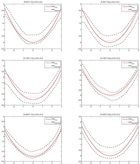
Figure 2. The fitting images and 95% confidence intervals of $\widehat{m}\left(z\right)$ with $\rho =0.2$ and $\lambda =0.2$.

4.2. Comparison of Results of Different Models

In this section, we will investigate the necessity of including nonparametric components, spatial correlation, and serial correlation if the real model is model (12). By deleting spatial correlation, serial correlation, and spatiotemporal correlations, respectively, in the model (12), we get the following three deleted models:

$$\begin{array}{c}\hfill \left\{\begin{array}{c}{y}_{it}=x_{it}^{\prime }\beta +m\left(z_{it}\right)+b_i+{\nu }_{it},\hfill \\ {\nu }_{it}=\lambda {\nu }_{i,t-1}+e_{it},\hfill \end{array}\right.\end{array}$$

(13)

$$\begin{array}{c}\hfill \left\{\begin{array}{c}{y}_{it}=x_{it}^{\prime }\beta +m\left(z_{it}\right)+b_i+{\epsilon }_{it},\hfill \\ {\epsilon }_{it}=\rho \sum _{j=1}^N{w}_{ij}{\epsilon }_{jt}+e_{it},\hfill \end{array}\right.\end{array}$$

(14)

$$\begin{array}{c}\hfill y_{it}=x_{it}^{\prime }\beta +m\left(z_{it}\right)+b_i+e_{it},\end{array}$$

(15)

where all variables in above models are the same as the model (12). To save space, we only study the case that $\rho =0.4$ and $\lambda =0.4$. In addition, we set $N=50,100$, $T=5$ and $mcn=2000$. By using PQML method in Section 2, the experimental results are presented in Table 5.

Table 5. Results of parametric estimates under the models (12)–(15).

		N = 50, T = 5					N = 100, T = 5
		$\widehat{\mathbf{\beta }}$	$\widehat{\mathbf{\rho }}$	$\widehat{\mathbf{\lambda }}$	${\widehat{\mathbf{\sigma }}}_{\mathbf{e}}^{\mathbf{2}}$	${\widehat{\mathbf{\sigma }}}_{\mathbf{b}}^{\mathbf{2}}$	$\widehat{\mathbf{\beta }}$	$\widehat{\mathbf{\rho }}$	$\widehat{\mathbf{\lambda }}$	${\widehat{\mathbf{\sigma }}}_{\mathbf{e}}^{\mathbf{2}}$	${\widehat{\mathbf{\sigma }}}_{\mathbf{b}}^{\mathbf{2}}$
model (12)	Mean	0.9848	0.4135	0.4092	1.0211	1.0576	1.0067	0.4063	0.4014	1.0128	1.0266
	MSE	0.0048	0.0014	0.0013	0.0015	0.0165	0.0023	0.0011	0.0009	0.0013	0.0125
	Mean	0.4711	-	0.5372	1.0221	1.1063	0.8424	-	0.5043	1.0331	1.1221
model (13)	MS	5.7078	-	0.0168	0.1057	0.1244	0.9135	-	0.0283	0.0095	0.1365
	$G{R}_1$(%)	118,812.5	-	1192.3	6946.7	653.9	39,617.3	-	3044.4	630.7	992
	Mean	0.8372	0.6462	-	1.0234	1.1322	0.9010	0.5968	-	1.0928	1.1012
model (14)	MSE	6.2135	0.1281	-	0.0171	0.1211	0.8845	0.1330	-	0.1013	0.1403
	$G{R}_1$(%)	129,347.9	9050	-	1040	633.9	38,356.5	11,990.9	-	7692.3	1022.4
	Mean	0.0366	-	-	1.0225	1.1123	0.9828	-	-	1.0948	1.1044
model (15)	MSE	5.8645	-	-	0.0160	0.1781	0.7981	-	-	0.1036	0.1474
	$G{R}_1$(%)	122,077.1	-	-	966.7	979.4	34,600	-	-	7869.2	1079.2

Table 5 reports Means, MSEs and $G{R}_1$s of parametric estimates in the models (12)–(15), where $G{R}_1$ is growth rate of MSE on the basis of that in model (12). From Table 5, we get the following conclusions: (1) the means of parametric estimates in the real model get closer to the true values as the sample size increases. However, we find that the means of estimates of ${\widehat{\sigma }}_e^2$ and ${\widehat{\sigma }}_b^2$ in model (13), ${\widehat{\sigma }}_e^2$ in the models (14) and (15) are very unstable, they do not converge to true values, respectively. Although the means of other parametric estimates get close to true values as the sample size increases, they still far away from true values and do not converge to true values. (2) In comparison with the real model, the MSEs of each parameter estimate in the deleted models increase. For most parametric estimates, they decrease with the increase in sample size except for $\widehat{\lambda }$ and ${\widehat{\sigma }}_b^2$ in the model (13), $\widehat{\rho }$, ${\widehat{\sigma }}_e^2$ and ${\widehat{\sigma }}_b^2$ in the model (14), ${\widehat{\sigma }}_e^2$ in the model (15). (3) The $G{R}_1$s of all parametric estimates are large, they do not decrease with the increase in sample size for some parametric estimates except for $\widehat{\beta }$ in the model (13)–(15) and ${\widehat{\sigma }}_e^2$ in the model (13).

Table 6 reports the medians and SDs of MADEs, $G{R}_2$s, and $G{R}_3$s for nonparametric estimates of the models (12)–(15), where $G{R}_2$ and $G{R}_3$ are growth rates of median and SD, respectively, on the basis of that in the model (12). It can be seen from Table 6 that, in comparison with the real model, the values of medians and SDs of MADEs for nonparametric estimates of the models (13)–(15) increase rapidly, and do not decrease with the increase in sample size.

Table 6. The medians and SDs of MADEs for nonparametric estimates under the models (12)–(15).

		Model (12)	Model (13)	Model (14)	Model (15)
N = 50, T = 5	Median	0.2232	0.7632	0.7259	0.7983
	$G{R}_2$(%)	(-)	(241.9)	(225.2)	(257.6)
	SD	0.1461	0.2857	0.3078	0.4305
	$G{R}_3$(%)	(-)	(95.5)	(1106.7)	(194.7)
N = 100, T = 5	Median	0.2042	1.2397	1.3323	1.2387
	$G{R}_2$(%)	(-)	(507.1)	(552.4)	(506.6)
	SD	0.1453	0.5595	0.4704	0.4810
	$G{R}_3$(%)	(-)	(285.1)	(223.7)	(231.0)

The above facts reveal that the efficiency of both parametric and nonparametric estimates depends on the correct specification of errors in (1)–(3), and violation of which can lead to inconsistency.

4.3. Performance of the Test

In this section, we aim to evaluate the power of hypothesis test proposed in Section 2.3. Consider the model (12), and the settings of $x_{it},b_i,w_{ij}$ and $e_{it}$ are the same as those in model (12). In addition, we only study the case that $\rho =0.2$ and $\lambda =0.2$. Then, the corresponding hypothesis is obtained as follows:

$$H_0:m\left(z_{it}\right)={\gamma }_0+{\gamma }_1{z}_{it}versus{H}_1:m\left(z_{it}\right)\ne {\gamma }_0+{\gamma }_1{z}_{it},$$

where $m\left(z_{it}\right)=\eta sin\left(\pi (z_{it}-0.5)\right)+0.8z_{it}+0.6$, $\eta$ are values consisting of $(0,0.05,0.1,0.2,0.5)$ and $z_{it}\sim U[0.2,1.6]$. In particular, when $\eta =0$, the above null hypothesis is exactly the true nonparametric function. As the value of $\eta$ increases, the true nonparametric function is increasingly farther from the null hypothesis. Figure 3 presents the true nonparametric functions with different $\eta$-values. In this section, we conduct simulations that N = 100, T = 8, 16 under significant levels $\alpha =0.01$ and 0.05, respectively. For each case, there are 1000 repetitions. Then, the powers of the hypothesis test are shown in Figure 4.

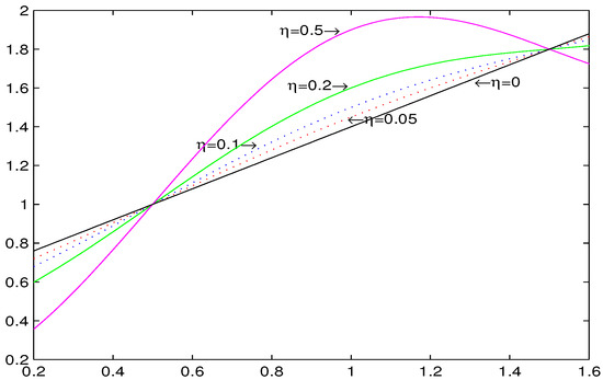
Figure 3. Trajectories of $m\left(z_{it}\right)$ with $\eta$ = 0, 0.05, 0.1, 0.2, and 0.5, respectively.

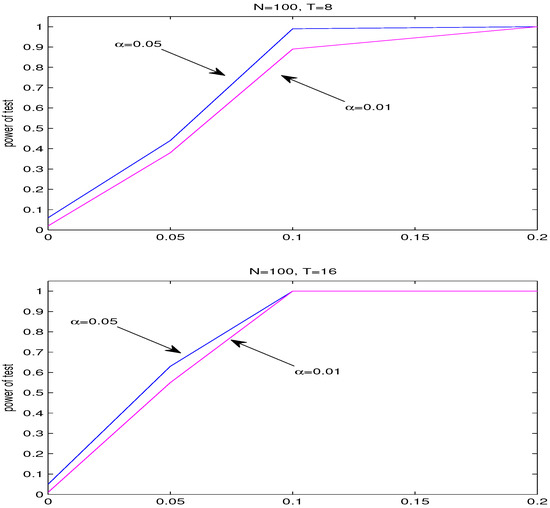
Figure 4. Powers of the test with $\alpha$ = 0.01 and 0.05, respectively, with sample size $N\ast T$.

We get from the Figure 4 and Table 7 that: (1) while $\eta$ = 0, the power of the test is very close to the significance level. As the value of $\eta$ increases, the power of the test statistic increases considerably, which indicates that our test statistic is sensitive to the alternative hypothesis of the proposed test problem. (2) While the number of spatial units is the same, the power of F-test with T = 16 is higher than that with T = 8. This shows that the F-test statistic performance get better as sample size increases.

Table 7. Powers of test with significance level $\alpha$.

N	T	$\mathit{\alpha }$	$\mathit{\eta }=0$	$\mathit{\eta }=0.05$	$\mathit{\eta }=0.1$	$\mathit{\eta }=0.2$	$\mathit{\eta }=0.5$
100	8	0.05	0.06	0.44	0.99	1	1
		0.01	0.02	0.38	0.89	1	1
100	16	0.05	0.05	0.63	1	1	1
		0.01	0.01	0.55	1	1	1

5. Real Data Analysis

In this section, we will illustrate the prescribed estimation and testing methods by Indonesian rice farming dataset with N = 171 and T = 6 which is a quintessential example of large N and small T in the stochastic frontier literature(see detail for Feng and Horrace [35]). This dataset has five variables, one response variable and four covariates. The response variable is natural logarithm of output of Indonesian rice farming, and the covariates include high, mixed, seed, and land, which are defined in Table 8. The dataset is from the agricultural economic research center of the Ministry of agriculture of Indonesia and compiled by the Agro Economic Survey. Based on the panel data of related variables of 171 farms over 6 growing seasons (three wet and three dry seasons), we will explore the influencing factors of output of Indonesian rice farming by RESPRM with separable space-time filters.

Table 8. Variables and their definitions.

Variable	Definition
high	Dummy variable for high yield varieties
	($high$ = 1 if the ith form at tth growing reason used high yield varieties,
	otherwise high = 0)
mixed	Dummy variable for mixed yield varieties
	(mixed = 1 if the ith form at tth growing reason used mixed varieties,
	otherwise mixed = 0)
seed	Seed weight used in tth season on ith farm(measured in kilogram)
land	Total area that farmers cultivated with rice(measured in hectares)

In order to take the proposed RESPRM with separable space-time filters to Indonesian rice farming dataset, we apply the F-test statistic proposed in Section 2.3 to verify whether or not a nonlinear relationship between covariates and response variable exists. The test results are given in Table 9. From Table 9, we find that land (other covariates) has (have) significant nonlinear (linear) relationship with natural logarithm of output of Indonesian rice farming at significant level $\alpha =0.01$.

Table 9. Results of F-test under significant level $\alpha =0.01$.

Variable	High	Mixed	Seed	Land
F-test value	2.33326	3.4298	3.7706	185.0233 ***

Note: *** means that it is significant under test level 1%.

Therefore, we consider the model (1)–(3), and set $1\le i\le 171$, $1\le t\le 6$, $y_{it}$ is the ith observation of $ln\left(rice\right)$ at tth growing season, $x_{it}$ are the ith observation of high, mixed, and seed at tth growing season, respectively, $z_{it}$ is land for the ith observation at tth growing season. $w_{ij}$ equals 1 if farms i and j are in the same village, equals 0 otherwise (see detail for Druska and Horrace [8]).

The parametric estimates results of the model (1)–(3) for fitting Indonesia rice farming data are described in Table 10. Via Table 10, we find that: (1) ${\beta }_i(i=1,2,3)>0$ show expectation of dummy variables for high, mixed, and seed have promotional effects on output of rice. (2) ${\sigma }_e^2=2.4049$ presents that the output of rice in different farm is relatively unstable and is affected by external fluctuations.

Table 10. Results of parametric estimates of model (1)–(3) for fitting Indonesia rice farming data.

Parameter	$\widehat{\mathit{\rho }}$	$\widehat{\mathit{\lambda }}$	${\widehat{\mathit{\beta }}}_1$	${\widehat{\mathit{\beta }}}_2$	${\widehat{\mathit{\beta }}}_3$	${\widehat{\mathit{\sigma }}}_{\mathit{e}}^2$	${\widehat{\mathit{\sigma }}}_{\mathit{b}}^2$
Estimate	−0.7227 ***	0.3891 ***	3.2123 ***	2.6885 ***	0.0172 **	2.4049 ***	0.0023 ***

Note: *** and ** mean that they are significant under test level 1% and 5% respectively.

Figure 5 shows the results of estimation and corresponding 95% confidence intervals of $m\left(z\right)$, where the blue solid line is the average fit over 500 simulations, the red and green dotted lines are the corresponding 95% confidence bands. From Figure 5, we know that land has obvious nonlinear effects on output of rice, and output of rice increases with the increase in land.

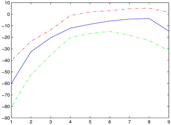
Figure 5. $\widehat{m}\left(z\right)$ and its 95% confidence intervals for the dataset of Indonesian rice farming in China.

6. Conclusions

In this paper, we study PQMLE and hypothesis test for RESPRM with separable space-time filters. The proposed model can simultaneously capture linear and nonlinear effects of covariates, spatial correlation of error structure, serial correlation of remainder error structure, and individual random effects. With the given conditional assumptions, asymptotic properties of PQMLE and asymptotic distribution of nonparametric components are proved. Monte Carlo simulations are applied to investigate the performance of estimators and test statistic under finite samples, and the results show that proposed estimators and test statistic are well-behaved under finite samples, and consistency of parametric estimates is hard to guarantee if spatial correlation and series correlation in the real model are ignored in some cases. In addition, the practicability of the proposed methods are also assessed by a real dataset.

This paper focuses only on RESPRM with separable space-time filters but does not account for spatially lagged response variables. How to extend our proposed estimation and testing methods to a random effects spatial lag semiparametric regression model with separable space-time filters is an open problem. In addition, we may combine generalized moment estimation method, quantile regression method and local linear method to estimate parametric and nonparametric components of the random effects spatial lag semiparametric regression model with separable space-time filters and RESPRM with separable space-time filters.

References

- Bates, G.E.; Neyman, J. Contributions to the theory of accident proneness II: True of false contagion. Univ. Calif. Publ. Statist. 1952, 1, 255–276. [Google Scholar]
- Chamberlain, G. Multivariate regression models for panel data. J. Econom. 1982, 18, 5–46. [Google Scholar] [CrossRef]
- Baltagi, B. Econometrics Analysis of Panel Data; Wiley Press: New York, NY, USA, 2001. [Google Scholar]
- Arellano, M. Panel Data Econometrics; Oxford University Press: New York, NY, USA, 2003. [Google Scholar]
- Baldev, R.; Baltagi, B. Panel Data Analysis; Springer Science & Business Media: Berlin/Heidelberg, Germany, 2012. [Google Scholar]
- Hsiao, C. Analysis of Panel Data; Cambridge University Press: Cambridge, UK, 2014. [Google Scholar]
- Elhorst, J. Spatial Econometrics: From Cross-Sectional Data to Spatial Panels; Springer Press: Berlin/Heidelberg, Germany, 2014. [Google Scholar]
- Druska, V.; Horrace, W. Generalized moments estimation for spatial panel data: Indonesian rice farming. Am. J. Agric. Econ. 2004, 86, 185–198. [Google Scholar] [CrossRef]
- Egger, P.; Pfaffermayr, M.; Winner, H. An unbalanced spatial panel data approach to US state tax competition. Econ. Lett. 2005, 88, 329–335. [Google Scholar] [CrossRef]
- Kapoor, M.; Kelejian, H.; Prucha, I. Panel data models with spatially correlated error components. J. Econ. 2007, 140, 97–130. [Google Scholar] [CrossRef]
- Lee, L.; Yu, J. Estimation of spatial autoregressive panel data models with fixed effects. J. Econ. 2010, 154, 165–185. [Google Scholar] [CrossRef]
- Elhorst, J. Serial and spatial autocorrelation. Econ. Lett. 2008, 100, 422–424. [Google Scholar] [CrossRef]
- Parent, O.; LeSage, J. A space-Ctime filter for panel data models containing random effects. Comput. Stat. Data Anal. 2011, 55, 475–490. [Google Scholar] [CrossRef]
- Lee, L.; Yu, J. Spatial penels: Random components versus fixed effects. Int. Econ. Rev. 2012, 53, 1369–1412. [Google Scholar] [CrossRef]
- Lee, L.; Yu, J. Estimation of fixed effects panel regression models with separable and nonseparable space-time filters. J. Econ. 2015, 184, 174–192. [Google Scholar] [CrossRef]
- Baltagi, B.; Song, S.; Jung, B.; Koh, W. Testing for serial correlation, spatial autocorrelation and random effects using panel data. J. Econ. 2007, 140, 5–51. [Google Scholar] [CrossRef]
- Cohen, J.; Morrison Paul, C. Public infrastructure investment, interstate spatial spillovers and manufacturing costs. Rev. Econ. Stat. 2004, 86, 551–560. [Google Scholar] [CrossRef]
- Zhao, J.; Zhao, Y.; Lin, J.; Miao, Z.-X.; Khaled, W. Estimation and testing for panel data partially linear single-index models with errors correlated in space and time. Random Matrices 2020, 9, 2150005. [Google Scholar] [CrossRef]
- Bai, Y.; Hu, J.; You, J. Panel data partially linear varying-coefficient model with both spatially and time-wise correlated errors. Stat. Sinica. 2015, 35, 275–294. [Google Scholar] [CrossRef]
- Shi, W.; Lee, L. Spatial dynamic panel data models with interactive fixed effects. J. Econ. 2017, 197, 323–347. [Google Scholar] [CrossRef]
- Baltagi, B.; Fingleton, B.; Pirotte, A. Estimating and forecasting with a dynamic spatial panel data model. Oxford. B Econ. Stat. 2014, 76, 112–138. [Google Scholar] [CrossRef]
- Cai, Z. Trending time-varying coefficient time series models with serially correlated errors. J. Econ. 2007, 136, 163–188. [Google Scholar] [CrossRef]
- Lin, X.; Carroll, R. Nonparametric function estimation for clustered data when the predictor is measured without/with error. J. Am. Stat. Assoc. 2000, 95, 520–534. [Google Scholar] [CrossRef]
- Fan, J.; Huang, T.; Li, R.Z. Analysis of longitudinal data with semi-parametric estimation of covariance function. J. Am. Stat. Assoc. 2007, 102, 632–641. [Google Scholar] [CrossRef]
- Fan, J.; Zhang, W. Statistical methods with varying coefficient models. Stat. Inference 2008, 1, 179–195. [Google Scholar] [CrossRef]
- Tang, L.; Liu, Y. Estimation of generalized spatial lag semi-parametric varying-coefficient panel model with random effects. Stat. Res. 2018, 35, 119–128. [Google Scholar]
- Fan, J.; Zhang, C.; Zhang, J. Generalized likelihood ratio statistics and Wilks phenomenon. Ann. Stat. 2001, 29, 153–193. [Google Scholar] [CrossRef]
- Su, L.; Jin, S. Profile quasi-maximum likelihood estimation of partially linear spatial autoregressive models. J. Econ. 2010, 157, 18–33. [Google Scholar] [CrossRef]
- Lee, L. Asymptotic distributions of quasi-maximum likelihood estimators for spatial autoregressive models. Econometrica 2004, 72, 1899–1925. [Google Scholar] [CrossRef]
- Hamilton, S.; Truong, Y. Local linear estimation in partly linear models. J. Multivar. Anal. 1997, 60, 1–19. [Google Scholar] [CrossRef]
- Ullah, A.; Su, L. Profile likelihood estimation of partially linear panel data models with fixed effects. Econ. Lett. 2006, 92, 75–81. [Google Scholar]
- Mack, Y.; Silverman, B. Weak and strong uniform consistency of kernel regression estimates. Zeitschrift für Wahrscheinlichkeitstheorie und Verwandte Gebiete 1982, 61, 405–415. [Google Scholar] [CrossRef]
- Su, L. Semiparametric GMM estimation of spatial autoregressive models. J. Econ. 2012, 167, 543–560. [Google Scholar] [CrossRef]
- Anselin, L. Spatial Econometrics: Methods and Models; Kluwer Academic Press: Dordrecht, The Netherlands, 1988. [Google Scholar]
- Feng, Q.; Horrace, W. Alternative technical efficiency measures: Skew, bias and scale. J. Appl. Economet. 2012, 27, 253–268. [Google Scholar] [CrossRef]
- White, H. Estimation, Inference and Specification Analysis; Cambridge University Press: New York, NY, USA, 1994. [Google Scholar]
- Kelejian, H.; Prucha, I. On the asymptotic distribution of the Moran I test statistic with applications. J. Econ. 2001, 104, 219–257. [Google Scholar] [CrossRef]
Publisher’s Note: MDPI stays neutral with regard to jurisdictional claims in published maps and institutional affiliations. |
© 2022 by the authors. Licensee MDPI, Basel, Switzerland. This article is an open access article distributed under the terms and conditions of the Creative Commons Attribution (CC BY) license (https://creativecommons.org/licenses/by/4.0/).