Abstract
A numerical method using combined detached-eddy simulation (DES) and a cavitation model considering the rotation effect is used for unsteady cavitation flow field of the centrifugal pump. A closed-type pump test system was established to obtain the pump performance and pressure pulsation characteristics under different flow rates and cavitation condition, which provide boundary conditions and verification of calculations. Based on the calculation results of the unsteady flow field of the centrifugal pump cavitation, the entropy generation analysis of the flow field and an analysis of the pressure fluctuation characteristics were carried out. Then, we tried to reveal the relationship between cavitation and the deterioration of the centrifugal pump performance and the generation of the unstable operation excitation force. The internal energy loss is mainly concentrated in the impeller, volute, and pump cavity area, which accounts for more than 85% of the total entropy generation. The characteristic frequency of a Strouhal number of about 0.333 appears at the volute tongue due to the cavitation flow spread downstream.
1. Introduction
Cavitation is a multiphase hydrodynamic phenomenon that occurs when the local static pressure of water is lower than the saturation vapor pressure [] at that prevailing temperature. Cavitation can lead to instability of the flow field structure, producing performance deterioration, which adversely affects the operation of centrifugal pumps. After cavitation appears, on the one hand, the bubbles consume energy and generate noise and vibration in the processes of generation and collapse. On the other hand, it interacts with the turbulence field []. It is interesting to analyze the characteristics of cavitation loss and pressure fluctuation of centrifugal pumps from the perspective of energy entropy generation.
Due to the complex structure of the centrifugal pump, it is difficult to directly process a cavitation observation inside the rotating impeller. Numerical simulation of cavitation on the basis of experimental verification is presently a hot topic []. Many scholars devote themselves to the research of the cavitation model. Schnerr [] et al. were devoted to modeling and analyzing compressible three-dimensional cavitating liquid flows with special emphasis on the detection of shock formation and propagation. Srinivasan et al. [] developed a novel cavitation-induced momentum-defect correction methodology to track cavitation zones and apply compressibility effects. Ji et al. [] and Huang et al. [] pay attention to cavitation–vortex interaction problems and use Large Eddy Simulation (LES) to solve the turbulence flow. Cheng et al. [] developed a new Euler–Lagrangian cavitation model for tip-vortex cavitation with the effect of non-condensable gas. Up to now, nearly one hundred cavitation models have been developed, and great progress has been made in capturing cavitation flow in simple structures in combination with LES, detached-eddy simulation, etc. However, LES is always limited by computing resource due to the large curvature of the centrifugal pump blade and its rotating characteristic. Wang et al. [] proposed a cavitation model considering rotation correction, and the unsteady cavitation characteristics of a centrifugal pump are studied with the Unsteady Reynolds-Averaged Navier–Stokes (URANS) method. Accurate prediction of the cavitation vortex field is still a difficult problem at present.
This study is devoted to establishing a numerical method by using a combined Detached Eddy Simulation (DES) and cavitation model considering the rotation effect []. Then, entropy generation analysis and pressure fluctuation analysis are used to study the flow loss and instability characteristics of the centrifugal pump under a cavitating condition.
2. Model and Methods
2.1. Pump Model and Test Rig
A commercial single-stage, single-suction, horizontal-orientated centrifugal pump from manufacturer Grundfos was used to process the study, whose casing is typically combined with a spiral vaneless volute. The designed working head and flowrate are required to be 20.6 m and 43 m3/h. The design parameters of the pump are shown in Table 1.

Table 1.
Hydraulic parameters of test pump.
A closed-type loop shown in Figure 1 was used to process the pump performance and cavitation characteristic measurement, which includes the water storage tank, vacuum pump, test pump, pipeline, and an electrical regulating valve. Water flowrate is measured by an electromagnetic flowmeter set between the upstream tank and the test pump. The pump is driven by a stable high-power motor, and a torque meter is installed between the motor and the pump. The electrical regulating valve is located at the downstream of the pump. The static pressure and dynamic pressure sensors are installed separately in the inlet and outlet pipelines of the pump. The compile acquisition program of LabVIEW 2019 software combined with the NI USB-6343 acquisition card is used to synchronously acquire the static pressure signal, dynamic pressure signal, liquid volume flow, speed, and torque. In order to obtain the cavitation characteristics of the pump under different flow rates, the vacuum is used to reduce the pump inlet pressure, while adjusting the opening of the valve to keep the pump flow constant in the meantime. Uncertainties of the measurement calculated by instrument precision are ±0.20% of flowrate, ±0.25% of pump head, and ±0.34% of pump efficiency. The test rig was built to give out the inlet and outlet boundary conditions for the next CFD approach. Moreover, the obtained pump performance data, such as the pump head and efficiency, are used to verify or modify the appropriate grid and the numerical calculation model.
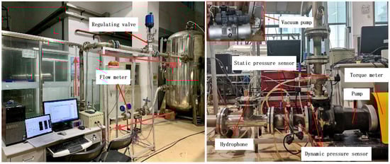
Figure 1.
Test rig.
2.2. Numerical Method
Three-dimensional modeling is carried out for the full flow path calculation domain of the test pump as shown in Figure 2. The calculation domain is composed of six parts, namely, the inlet pipe, the impeller ring, the impeller, the pump chamber, the volute, and the outlet pipe. The extension with five times the pipe diameter is processed to maintain the stability of the fluid flow in the inlet and outlet parts so as to improve the accuracy of the numerical simulation.
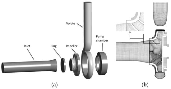
Figure 2.
Three-dimensional view of computing domain and grid results. (a) Computing domain (b) Mesh.
The structured type of meshes are used for grid generation and are specially densified at areas with complex flow structures such as the blade wall. In addition, grid independence verification is processed to balance calculation accuracy and simulation time. The results show that the relative errors of head and efficiency are less than 1% when the number of grids is more than 6.342 million. And the y+ value of the near wall grid is less than 5, which can meet the simulation requirements of pump cavitation.
The shear stress transport (SST) turbulence model embedded in ANSYS CFX 17.2 software (ANSYS, Inc., Canonsburg, PA, USA) was repeatedly used for steady calculation. Then, the unsteady simulation was processed based on the DES method. It switches from the SST-RANS model to the LES model in regions where the turbulent length, Lt, predicted by the RANS model is larger than the local mesh spacing. The actual formulation for a two-equation model is given below.
where Pk is the production of the turbulent kinetic energy; ρ is density; t is time; k is turbulent kinetic energy; ω is the specific dissipation rate; σk and σω are model constants; μ is the dynamic viscosity property; and μt is the turbulent eddy viscosity.
In this case, the length scale calculating the dissipation rate in the equation for the turbulent kinetic energy is replaced by the local mesh. As the grid is refined below the following limit, the DES limiter is activated and switches the model from the RANS to the LES mode.
where x, y, z means three directions of the spatial coordinate system for the local computational cell. ε is the turbulent dissipation rate. β* are model constants. This model allows the user to avoid the high computing costs of covering the wall boundary layers in the LES mode. In order to avoid the limitation of grid refinement inside attached boundary layers, the dissipation term in the k-equation is thereby re-formulated as follows:
The numerical formulation is also switched between an upwind biased and a central difference scheme in the RANS and DES regions, respectively.
A rotating-based Zwart–Gerber–Belamri (RZGB) cavitation model is used for the numerical simulation of cavitating flow inside the pump. This model could consider the rotating effect and geometric characteristics of the impeller, which is based on the Zwart–Gerber–Belamri cavitation model. The expressions of the evaporation source term and condensation source term are as follows:
where rnuc represents the volume fraction of cavitation nuclei, rnuc = 5 × 10⁻⁴; RB represents the cavitation radius, RB = 1 × 10⁻⁶ m; Cwap and Ccond represents the evaporation coefficient and condensation coefficient, respectively.
The inlet boundary is set with total pressure; the outlet boundary condition is selected for mass flow; the working medium is 25 °C clear water; the saturated steam pressure of water is set to 3169 Pa; and the convergence accuracy is set to 10−5. An appropriate time step Δt is set to 0.00017182 s, which satisfies the time-step independence after judging by the Courant number calculation. The default value of the software is adopted in the calculation.
The head coefficient is defined as follows.
where the g means the gravity; H represents head; and u2 is the rotating speed.
2.3. Data Reduction Method
An entropy generation analysis method is proposed based on the second law of thermodynamics, which combines heat transfer and fluid mechanics to analyze energy loss. The energy dissipation will inevitably occur in the cavitation flow process of the test pump, which is closely connected to pump performance and instability. The definitions of direct dissipative entropy production rate and turbulent dissipative entropy production rate are followed, respectively.
where “-” represents the time average term, is the direct dissipative entropy production rate, “′” represents the pulsation term, indicates the turbulent dissipation entropy production rate, and .
Because it is difficult to directly calculate the entropy production rate caused by fluctuating velocity, a method proposed by Kock and Herwig [] is adopted in this paper to correlate the ω value in the turbulence model with the entropy production rate generated by the fluctuating velocity component.
where β = 0.09; ω indicates the turbulent eddy viscosity frequency, s−1; and k is the turbulent kinetic energy, m2/s2. The direct dissipative entropy generation and turbulent dissipative entropy generation can be obtained by volume integration of the computational domain based on this equation. In addition, wall entropy generation also accounts for a large proportion of losses. However, the calculation error of entropy generation near the wall is large with the direct dissipative entropy generation formula because the medium is viscous, and there is a large velocity gradient in the boundary layer. Therefore, in this study, the wall entropy generation is calculated by the surface integral method [].
where indicates the wall entropy rate, is the wall entropy, and indicates wall shear stress, Pa. represents the surface area of the computational domain, m2. is the velocity vector of the fluid at the center of the first layer mesh, m/s.
3. Results Analysis
3.1. Experimental Verification of Pump Performance
Figure 3a shows the comparison results of pump performance at 2910 r∙min−1 between the experiment and CFD under different flowrates. It can be seen from the comparison that the trend of the measurement results is in good agreement with the simulation over the whole range of flowrates. Under the design flow rate, the measured head of the test pump is 22.02 m, and the numerical simulation result is 22.90 m, with a relative error of 3.99%. Moreover, the measured efficiency of the test pump is 72.65%, and the numerical simulation result is 75.47%, with a relative error of 3.88%. As seen in Figure 3b, the head coefficient of the test pump starts to decrease significantly at 2910 r∙min−1 and 43 m³/h, when the cavitation number decreases to about 0.09 both in the experiment and numerical simulation, while the head drops by 3% when the cavitation number decreases to 0.06. The predicted results of RZGB cavitation model are closer to the test results, which indicates that the selected turbulence model, cavitation model, and boundary condition setting for CFD are reliable.

Figure 3.
Comparison between numerical simulation and experimental results. (a) Pump performance curves. (b) Pump cavitation characteristic curves.
3.2. Entropy Generation Analysis
Figure 4 shows the distribution of the three production terms of entropy generation defined in previous section under different cavitation number, where the blue color values are calculated from Equation (7), the grey color values are calculated from Equation (5), and the red color values are calculated from Equation (8). It can be seen that the sum of the three types of entropy increases with the decrease in cavitation number. This is because, along with the development of cavitation, the number and volume of cavitation bubbles inside the impeller will also increase until the channel is blocked, which brings loss in the whole process. With a decrease in cavitation number, the total entropy generation increases a little, while the values increase by 0.5 W/K from σ = 0.43 to 0.051. It indicates that the development of cavitation has little influence on the pump efficiency. Under different cavitation numbers, the turbulent dissipation entropy value is greater than the wall entropy value. Therefore, the turbulence dissipation entropy generation and wall entropy generation play an important role in the flow loss of the test pump.
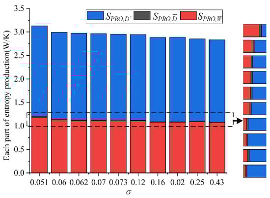
Figure 4.
The distribution of entropy generation with different cavitation numbers.
In order to further analyze the internal energy loss of the test pump under cavitation condition, the entropy generation at five parts of the flow passage are calculated under different cavitation numbers. Figure 5 shows the proportion of entropy generation under three cavitation numbers, i.e., σ = 0.43 means no cavitation, σ = 0.07 indicates the condition that the pump head dropped by 1%, and σ = 0.06 indicates the condition that the pump head dropped by 3%. The areas with large energy losses are mainly concentrated in the volute, impeller, and pump chamber areas, which account for more than 85% of the total entropy generation. The entropy generation of the volute area accounts for almost 50% of the total entropy generation, and the entropy generation of the impeller area and the pump chamber area is close. In general, the entropy generation upstream of the inlet pipe is the smallest. However, it is worth noting that the entropy generation in the impeller eye area accounts for about 10% of the total entropy generation even though the leakage is small compared with the other flow passage.
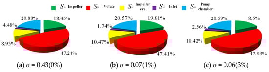
Figure 5.
Proportion of entropy production under different cavitation numbers.
Figure 6 shows the distribution of the entropy production rate at middle section of the test pump under three typical cavitation numbers. The entropy production rate is mainly distributed on the blade wall and impeller flow passage, volute wall and volute flow passage, pump cavity wall, pump cavity flow passage, and annular gap for all cavitation development levels. With the decrease in cavitation number, the entropy yield of the inlet extension section tends to decrease, while that of other flow passage components tends to increase.
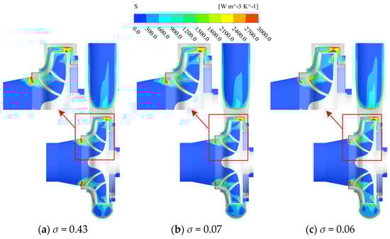
Figure 6.
The distribution of entropy production at middle section of pump channel.
3.3. Analysis of Pressure Fluctuation Characteristics
In order to study the pressure pulsation characteristics of the test pump under different cavitation developments, six monitoring points (Pre1~Pre6) are set at span = 0.5 on the blade pressure surface, which aims to avoid pressure disturbance from the cavitation bubble. In addition, seven monitoring points (Vol1~Vol7) are set at the middle section of the volute, as shown in Figure 7. Pre3 is set at the inlet blade throat of the impeller, which is the narrowest part of the flow passage. In particular, the Strouhal number corresponding to the shaft passing frequency is StR = fR/fBPF = 0.1667, and the Strouhal number corresponding to the blade passing frequency is StR = fR/fBPF = 1. The pressure pulsation coefficient of each monitoring point on the blade pressure surface is obtained by dimensionless processing of the pressure pulsation at each monitoring point []. The data of the last 10 cycles are taken for a fast Fourier transform to obtain the corresponding frequency domain of the pressure pulsation coefficient at each monitoring point.
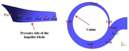
Figure 7.
The distribution of pressure pulsation monitoring points.
It can be seen from Figure 8 that the pressure fluctuation coefficient signals show discrete frequency domain characteristics with the development of cavitation for all monitoring points. Due to the different development of cavitation structure in each flow channel, the dominant frequency is always the fR (shaft passing frequency), especially for monitoring points that are far away from the volute tongue, such as Pre1 and Pre2. Correspondingly, the monitoring points that are relatively close to the volute tongue, such as Pre5 and Pre6, have a main frequency of fR; other frequencies are its multiples. The amplitude gradually increases as the distance between the points and the volute tongue gets closer, when σ = 0.43 and 0.07. However, the amplitude of Pre3 also presents higher values when σ = 0.06 and 0.051, which might be due to the location. When cavitation develops seriously, a large number of cavities on the suction side affects the pressure fluctuation characteristic. In addition, there are more low-frequency pulsations at each monitoring point when σ = 0.43, while there are fewer low-frequency pulsations characteristic for Pre1, Pre2, and Pre3 at the severe cavitation stage when σ = 0.06 and 0.051. In the critical cavitation state σ = 0.06, the Pre3 and Pre4 have a brand frequency characteristic between St = 0.075 and 0.9, which is related to the cavitation shedding frequency and is determined by the chord width and length of the blade inlet. This frequency is helpful for pump cavitation monitoring because the pump head starts to drop more steeply at this condition.
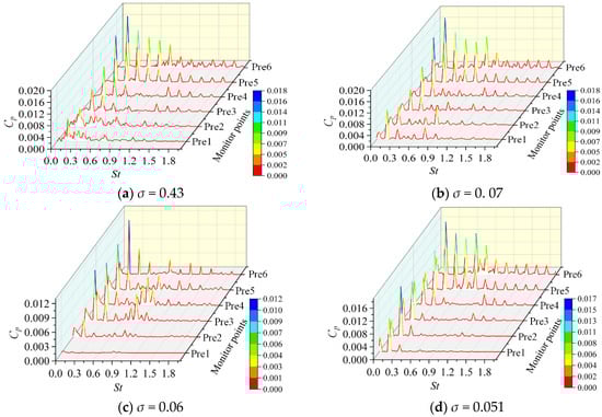
Figure 8.
Frequency domain of pressure pulsation coefficient at each monitoring point on blade pressure surface under different cavitation numbers.
The typical cavitation condition σ = 0.06 is selected to analyze the pressure fluctuation characteristics of each monitoring point in the middle section of the volute. Seen from the time domain diagram of Figure 9, the pressure pulsation coefficient of each monitoring point has six obvious “peaks and valleys” in a rotation cycle, and the amplitude and phase of the pressure pulsation coefficient also have obvious differences. The reason for the phase difference is that the time of blade sweeping the monitoring points starting from Vol1 to Vol6 are different. The change rate and amplitude of the pressure pulsation coefficient at Vol2 and Vol1 are the largest, while that at Vol3, Vol4, Vol5 and Vol6 are obviously smaller. On the one hand, the monitoring points are gradually farther away from the diaphragm, which weakens the dynamic and static interference between the blade and the volute. On the other hand, the area of the section of monitoring point locating is gradually increased, making the average cavity volume of the same mass cavity decrease in each cross-section. Under the combined action of the two factors, the amplitude of the pressure fluctuation coefficient shows a trend of gradual reduction. However, the change rate and amplitude of the pressure fluctuation coefficient at Vol7 are also bigger, because the monitoring point is also relatively close to the tongue, which is affected by the dynamic and static interference between the blade and the volute. Frequency domain results in Figure 9b show that the pressure pulsation coefficient signals at each monitoring point show discrete frequency domain characteristics. The dominant frequency of the pressure pulsation coefficient is located at the blade passing frequency and the multiple, and the maximum peak is always located at the blade passing frequency. The dynamic–static interference between the blades and the pump tongue results in higher pressure pulsation at two monitoring points, Vol1 and Vol2, located near this area. There is a frequency of about 0.333StBPF appearing at the Vol1 monitoring point, which is mainly caused by the strong three-dimensional unsteady cavitation flow.
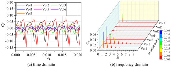
Figure 9.
Time domain and frequency domain diagrams of pressure pulsation in the volute.
4. Conclusions
- (1)
- Unsteady cavitation flow of the centrifugal pump was calculated by combined DES and RZGB cavitation models; then, the entropy generation analysis of the flow field and the pressure fluctuation characteristics were carried out. The main conclusions are as follows:
- (2)
- Under different cavitation numbers, the turbulent dissipative entropy generation and wall entropy generation play an important role in the flow loss of the pump, while the viscous dissipative entropy generation is very small and can even be ignored. The sum of the three types of entropy output values increases with the decrease in cavitation numbers. The internal energy loss is mainly concentrated in the impeller, volute, and pump cavity areas, which account for more than 85% of the total entropy generation. The impact between the leading edge of the blade and the incoming flow, as well as the dynamic and static interference between the blade outlet and the volute tongue, are the main reasons for the flow loss in the impeller area.
- (3)
- In the non-cavitation stage and cavitation development stage, there are many low-frequency pulsations at each monitoring point. When the cavitation number decreases to 0.06, the expansion of the cavitation volume will absorb part of the pressure pulsation, resulting in a decrease in the amplitude of the pressure pulsation coefficient at the Pre6 monitoring point compared with the previous cavitation stage. The Pre3 and Pre4 has a brand frequency characteristic between St = 0.075 and 0.9. The characteristic frequency of about 0.333 StBPF appears at Vol1, which is mainly caused by the strong three-dimensional unsteady cavitation flow. In the initial cavitation stage and the severe cavitation stage, the low-frequency pulsations are reduced. The position of the monitoring point with large pressure fluctuation amplitude is consistent with large wall entropy generation.
Author Contributions
Conceptualization, Q.S. and M.L.; methodology, M.L.; software, F.D. and Y.L.; validation, F.D. and S.Y.; formal analysis, M.L.; investigation, F.D.; resources, M.L.; data curation, F.D.; writing—original draft preparation, F.D.; writing—review and editing, Q.S. and S.Y.; visualization, M.L.; supervision, S.Y.; project administration, S.Y.; funding acquisition, Shouqi Yuan. All authors have read and agreed to the published version of the manuscript.
Funding
The paper is supported from the National Natural Science Foundation of China (51976079), the National Key R&D Program of China (2020YFC1512403), Research Project of State Key Laboratory of Mechanical System and Vibration (MSV202201), and Postgraduate Research & Practice Innovation Program of Jiangsu Province (KYCX22_3647).
Institutional Review Board Statement
Not applicable.
Informed Consent Statement
Not applicable.
Data Availability Statement
Data are contained within the article.
Conflicts of Interest
Author Minquan Liao was employed by the company Gansu Water Conservancy and Hydropower Survey Design and Research Institute Co., Ltd. The remaining authors declare that the research was conducted in the absence of any commercial or financial relationships that could be construed as a potential conflict of interest.
Abbreviations
| b2 | impeller outlet width | n | rotate speed |
| Cp | Pressure fluctuation coefficient, | ns | specific rotate speed |
| Ds | pump inlet diameter | average pressure | |
| Dd | pump outlet diameter | pv | Saturated pressure |
| D1 | impeller inlet diameter | ρl | density |
| D2 | impeller outlet diameter | pin | pressure at the pump inlet |
| σ | cavitation number, | Q | flow rate |
| η | efficiency | u1 | tangential velocity at the impeller inlet |
| f | frequency | u2 | tangential velocity at the impeller outlet |
| H | head | Ψ | head coefficient |
| Hd | Design head | z | blade number of impeller |
| n | rotational speed |
References
- Bachert, R.; Stoffel, B.; Dular, M. Unsteady Cavitation at the Tongue of the Volute of a Centrifugal Pump. J. Fluids Eng. Trans. ASME 2010, 132, 061301. [Google Scholar] [CrossRef]
- Reuter, F.; Gonzalez-Avila, S.R.; Mettin, R.; Ohl, C.D. Flow fields and vortex dynamics of bubbles collapsing near a solid boundary. Phys. Rev. Fluids 2017, 2, 064202. [Google Scholar] [CrossRef]
- Fu, Y.; Yuan, J.; Yuan, S.; Pace, G.; d’Agostino, L.; Huang, P.; Li, X. Numerical and Experimental Analysis of Flow Phenomena in a Centrifugal Pump Operating Under Low Flow Rates. J. Fluids Eng. Trans. ASME 2015, 137, 011102. [Google Scholar] [CrossRef]
- Schnerr, G.H.; Sezal, I.H.; Schmidt, S.J. Numerical investigation of three-dimensional cloud cavitation with special emphasis on collapse induced shock dynamics. Phys. Fluids 2008, 20, 040703. [Google Scholar] [CrossRef]
- Srinivasan, V.; Salazar, A.J.; Saito, K. Numerical simulation of cavitation dynamics using a cavitation-induced-momentum-defect (CIMD) correction approach. Appl. Math. Model. 2009, 33, 1529–1559. [Google Scholar] [CrossRef]
- Ji, B.; Luo, X.; Arndt, R.E.; Wu, Y. Numerical simulation of three dimensional cavitation shedding dynamics with special emphasis on cavitation-vortex interaction. Ocean Eng. 2014, 87, 64–77. [Google Scholar] [CrossRef]
- Huang, B.A.; Zhao, Y.; Wang, G.Y. Large Eddy Simulation of turbulent vortex-cavitation interactions in transient sheet/cloud cavitating flows. Comput. Fluids 2014, 92, 113–124. [Google Scholar] [CrossRef]
- Cheng, H.; Long, X.; Ji, B.; Peng, X.; Farhat, M. A new Euler-Lagrangian cavitation model for tip-vortex cavitation with the effect of non-condensable gas. Int. J. Multiph. Flow 2021, 134, 103441. [Google Scholar] [CrossRef]
- Jian, W.; Yong, W.; Houlin, L.; Qiaorui, S.; Dular, M. Rotating Corrected-Based Cavitation Model for a Centrifugal Pump. J. Fluids Eng. Trans. ASME 2018, 140, 111301. [Google Scholar] [CrossRef]
- Si, Q.; Deng, F.J.; Lu, Y.; Liao, M.Q.; Yuan, S.Q. Unsteady Cavitation Analysis of the Centrifugal Pump Based on Entropy Production and Pressure Fluctuation. In Proceedings of the 15th European Turbomachinery Conference, paper n. ETC2023-254, Budapest, Hungary, 24–28 April 2023; Available online: https://www.euroturbo.eu/publications/conference-proceedings-repository/ (accessed on 6 June 2023).
- Kock, F.; Herwig, H. Local entropy production in turbulent shear flows: A high-Reynolds number model with wall functions. Int. J. Heat Mass Transf. 2004, 47, 2205–2215. [Google Scholar] [CrossRef]
- Wang, C.; Zhang, Y.; Hou, H.; Zhang, J.; Xu, C. Entropy production diagnostic analysis of energy consumption for cavitation flow in a two-stage LNG cryogenic submerged pump. Int. J. Heat Mass Transf. 2019, 129, 342–356. [Google Scholar] [CrossRef]
- Zhang, N.; Zheng, F.; Liu, X.; Gao, B.; Li, G. Unsteady flow fluctuations in a centrifugal pump measured by laser Doppler anemometry and pressure pulsation. Phys. Fluids 2020, 32, 125108. [Google Scholar] [CrossRef]
Disclaimer/Publisher’s Note: The statements, opinions and data contained in all publications are solely those of the individual author(s) and contributor(s) and not of MDPI and/or the editor(s). MDPI and/or the editor(s) disclaim responsibility for any injury to people or property resulting from any ideas, methods, instructions or products referred to in the content. |
© 2023 by the authors. Licensee MDPI, Basel, Switzerland. This article is an open access article distributed under the terms and conditions of the Creative Commons Attribution (CC BY-NC-ND) license (https://creativecommons.org/licenses/by-nc-nd/4.0/).