Design of Identification System Based on Machine Tools’ Sounds Using Neural Networks

Abstract

Recently, deep learning models such as convolutional neural networks (CNNs), convolutional autoencoders (CAEs), CNN-based support vector machines (SVMs), YOLO, fully convolutional networks (FCNs), fully convolutional data descriptions (FCDDs) and so on have been applied to defect detections and anomaly detections of various kinds of industrial products, materials and systems. In those models, downsampled images, including target features, are used for training and testing. On the other hand, although various types of anomaly detection systems based on time series data such as sounds and vibrations are also applied to manufacturing processes, complicated conversions to the frequency domain are basically needed in conventional approaches. This paper addresses an important industrial problem for detecting anomalies in machine tools at low cost using audio data. Intelligent anomaly diagnosis systems for computer numerical control (CNC) machine tools are considered and proposed, in which raw time-series data without the need of conversion to the frequency domain can be directly used for training and testing. As for the NN models for comparison, conventional shallow NN, RNN and 1D CNN are designed and trained using the nine kinds of mechanical sounds. Classification results of test sound block (SB) data by the three models are shown. Then, an autoencoder (AE) is designed and considered for the identifier by training it using only normal SB data of a machine tool. One of the technical needs in dealing with time-series data such as SB data by NNs is how to clearly visualize and understand anomalous regions in concurrence with identification. Finally, we propose the SB data-based FCDD model to meet this need. Basic performance of the SB data-based FCDD model is evaluated in terms of anomaly detection and concurrent visualization of understanding.

1. Introduction

Due to the declining birthrate and aging population, the number of skilled workers in Japan’s manufacturing industry is decreasing, resulting in a serious labor shortage. In product inspection processes, there is an ever-increasing need to automate the task of detecting defective products, which has traditionally been achieved visually by human eyes. In order to solve the issues related to product quality control faced by the manufacturing industry, the authors are developing an application that can easily and effectively design and train a machine learning model that has the same or more ability to identify defective products as skilled inspectors. 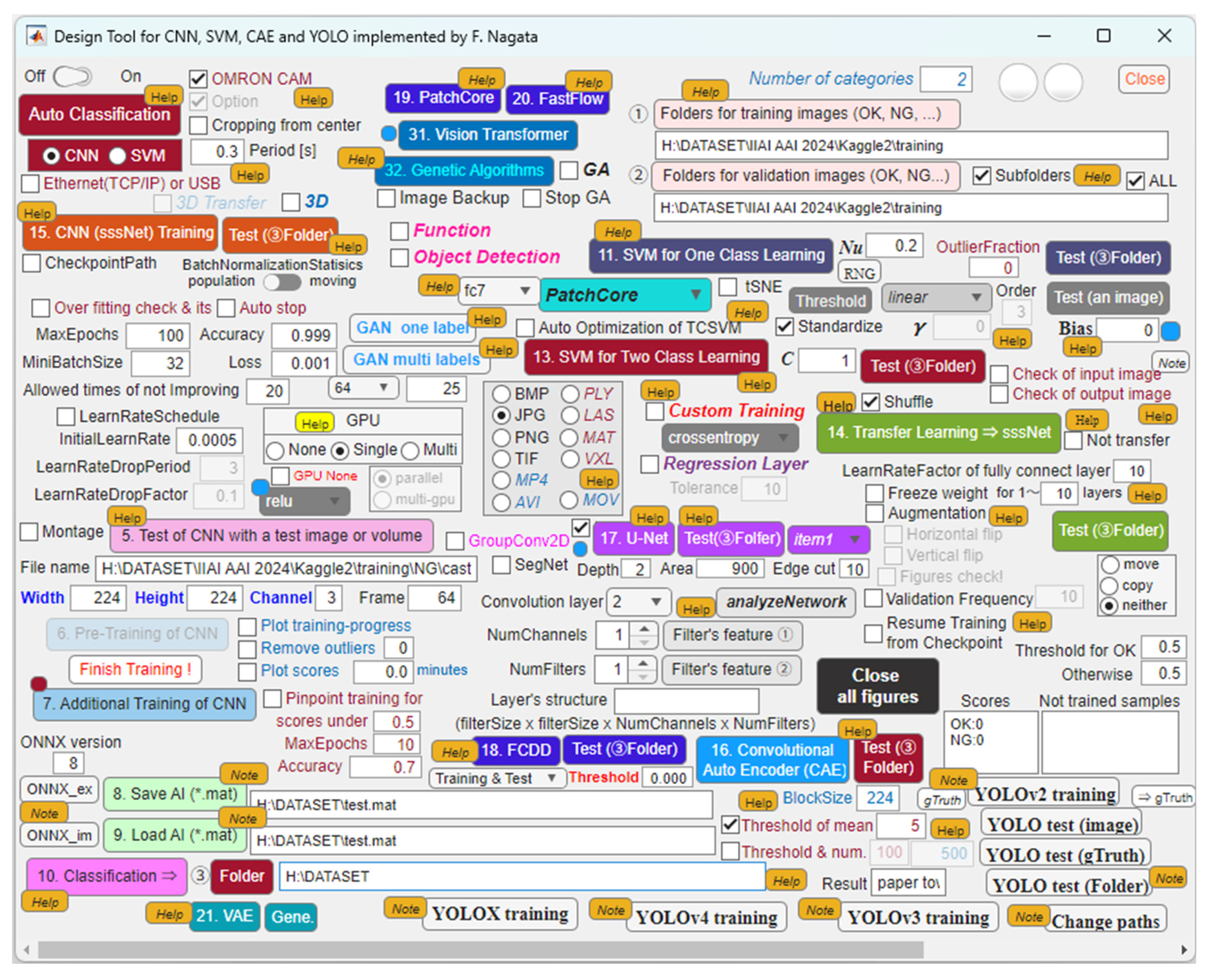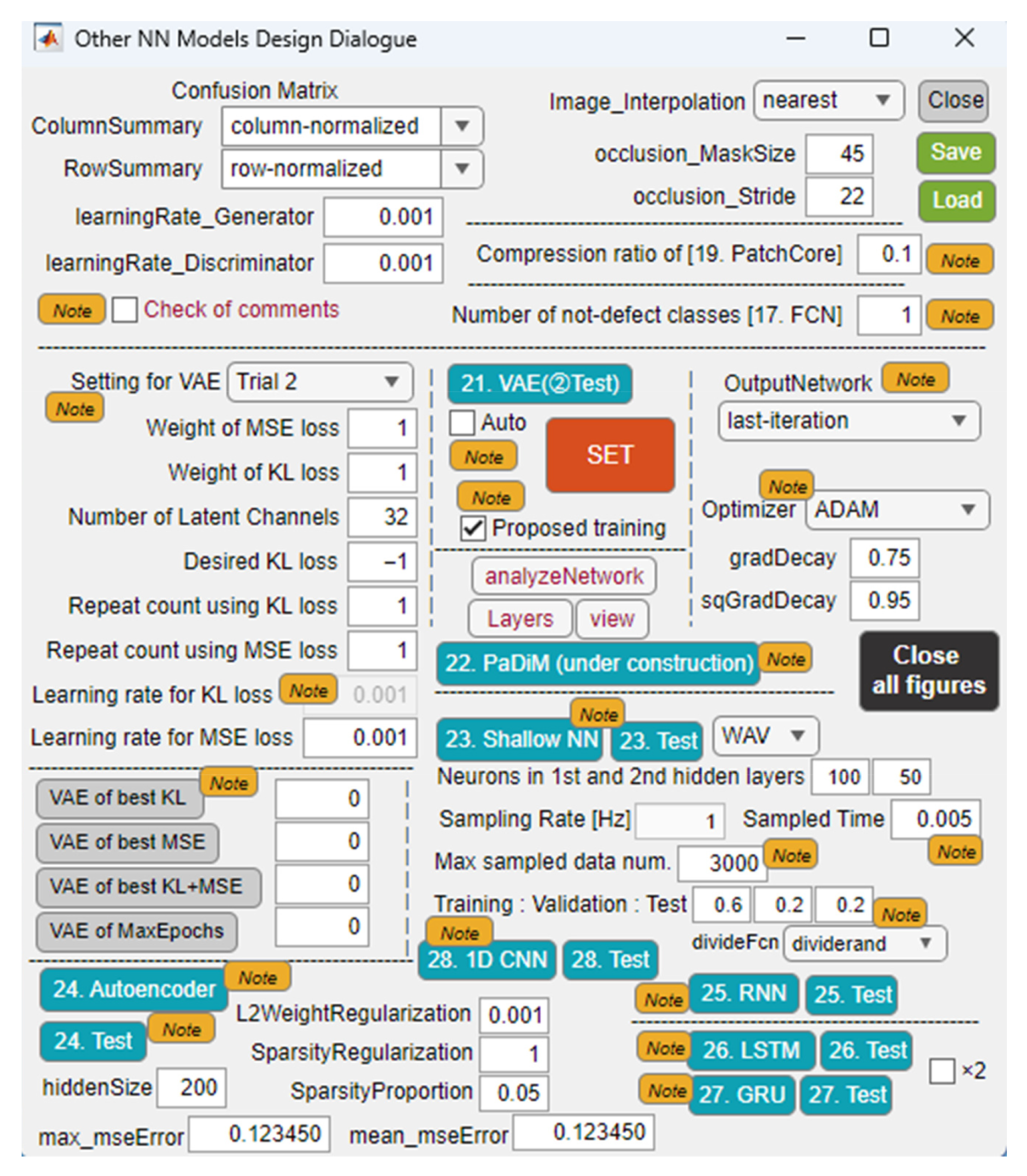Figure 1 and Figure 2 show the main and sub dialogs developed on MATLAB R2025a. By using the proposed application, the authors are supporting engineers to build their desired machine learning models for defect detection of industrial products and materials included in images and movies. Available models are convolutional neural network (CNN), convolutional autoencoder (CAE), support vector machine (SVM), you look only once (YOLO) [1,2], U-Net, segmenting objects by locations (SOLO) [3,4], mask region-based CNN (Mask R-CNN) [5], fully convolutional data description (FCDD) and so on [6]. In fact, in manufacturing industries, there is a strong need for flexible anomaly detection systems that allow workers to easily cope with all the processes from setting up the environment to operating the system so that we are evaluating and improving the application through trial use and expanding functionality based on feedback from users.

Figure 1. Main dialog developed on the MATLAB R2025a system for the user-friendly design of CNN, SVM, CAE, FCDD, and so on.

Figure 2. Another dialog to user-friendly design of shallow NN, RNN, VAE, 1D CNN, and so on.

Up to now, much relevant research on anomaly detection systems based on sound data has been proposed. However, when monitoring the operating status of CNC machine tools and other equipment based on time series data, there does not seem to be sufficient discussion about anomaly detection and concurrent visualization of prediction. In addition, many systems require preprocessing, such as converting time-domain data into the frequency domain. For example, Harada et al. proposed a baseline system for first-shot-compliant unsupervised anomaly detection for machine condition monitoring, in which a simple autoencoder-based implementation combined with a selective Mahalanobis metric is implemented as a baseline system. The performance is evaluated to set the target benchmark for the forthcoming Detection and Classification of Acoustic Scenes and Events (DCASE2023T2) [7]. Zhou et al. proposed an incremental learning-based anomaly sound detection model that enhances the model’s capacity to learn from continuous data streams, reduces knowledge forgetting, and improves the stability of the model in the anomaly sound detection task. Experiments using Task 2 data from the DCASE2020 challenge show that the proposed method effectively improves the average AUC and average pAUC by 7% to 10% when compared to the fine-tuning strategy [8]. Also, Dong et al. proposed a self-encoder model combining a residual CNN and a long and short-term memory (LSTM) network to extract features in both spatial and temporal dimensions, respectively, to make full use of the information of the audio signal [9]. In addition, Sekhar et al. proposed texture analysis-based transfer learning CNN models so that they can be applied to a three-class (high/medium/low tool wear) classification task of tool wear based on the noise generated during mild steel machining. Machining acoustics were converted to spectrogram images so that they can be given to the input layer of each CNN, in which four pre-trained models, SqueezeNet, ResNet50, InceptionV3, and GoogLeNet, were used for the backbone. More recently, Liao et al. proposed an enhanced contrastive ensemble learning method for anomaly sound detection, in which the log-mel transform for frequency domain feature analysis and the Mel spectrogram are used to represent the features of the statistical domain [10]. It is reported that the method is effective in automatically monitoring the operating conditions of the production equipment by detecting the sounds emitted by the machine.

It is known that spectrograms, MFCCs (Mel-Frequency Cepstrum Coefficients), and Mel-spectrograms are promising practices for audio analysis. For example, Abdul and Al-Talabani reported that MFCCs have been designed to model features of audio signals and have been widely used in various fields. MFCCs are one of the most widely used features in speech recognition and speech processing. Their research aimed to review the applications that the MFCC has been used for in addition to some issues that were facing the MFCC computation and its impact on the model performance [11]. Dossou and Gbenou used mel-spectrograms over conventional MFCCs features and assessed the abilities of CNNs to accurately recognize and classify emotions from speech data. Their designed speech emotion recognition model trained on four valid speech databases achieved a high classification accuracy of 95.05%, over eight different emotion classes: anger, anxiety, calm, disgust, happiness, neutral, sadness, and surprise [12]. Also, Islam and Tarique considered two spectral images of voice signals called spectrograms and mel-spectrograms to detect dysphonic voices. It is known that the spectrogram is a convenient representation of voice signals on a time-frequency scale and has been popularly investigated in pathological voice detection algorithms. It is reported from simulation results that the mel-spectrogram was superior to the spectrogram in terms of classification accuracy [13]. Furthermore, Ninevski et al. proposed a new approach to analyze acoustic emission data in the phase domain. In addition, the use of psychoacoustics was evaluated. Both approaches were applied to monitoring the condition of a CNC milling tool [14]. However, when the above approaches are applied, it seems that raw time-series sound data must be transformed into frequency domain.

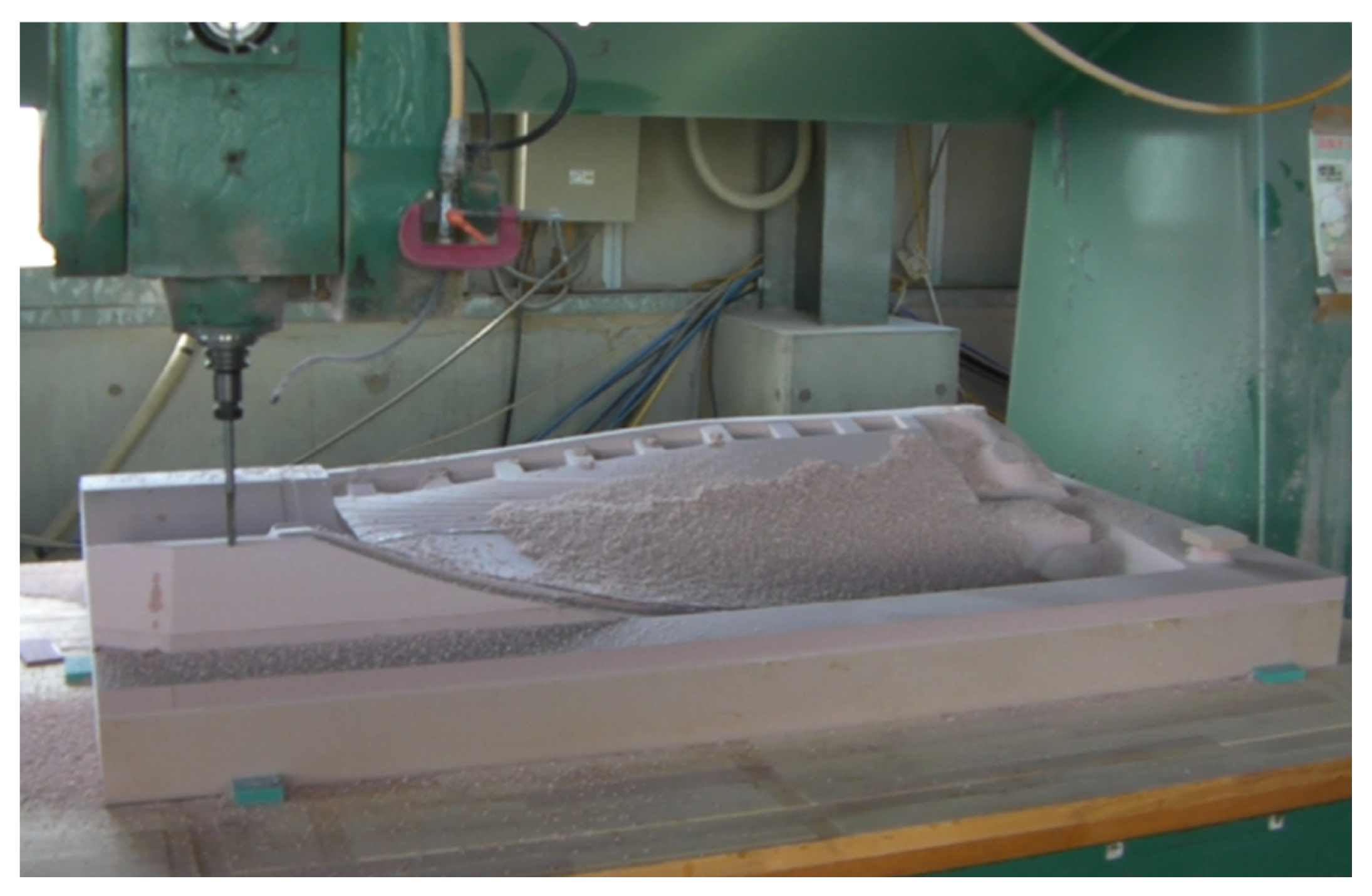
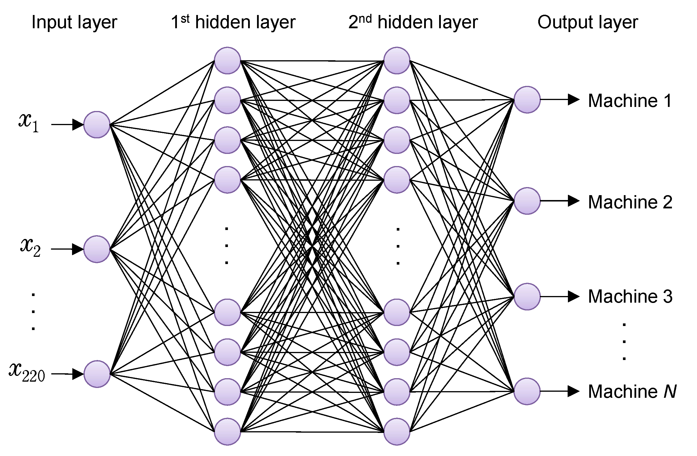
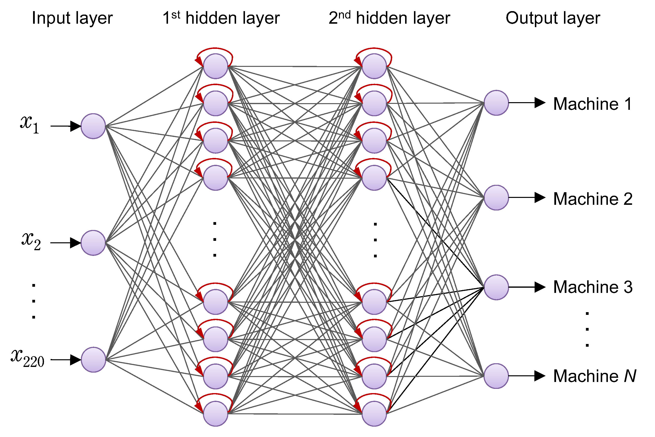
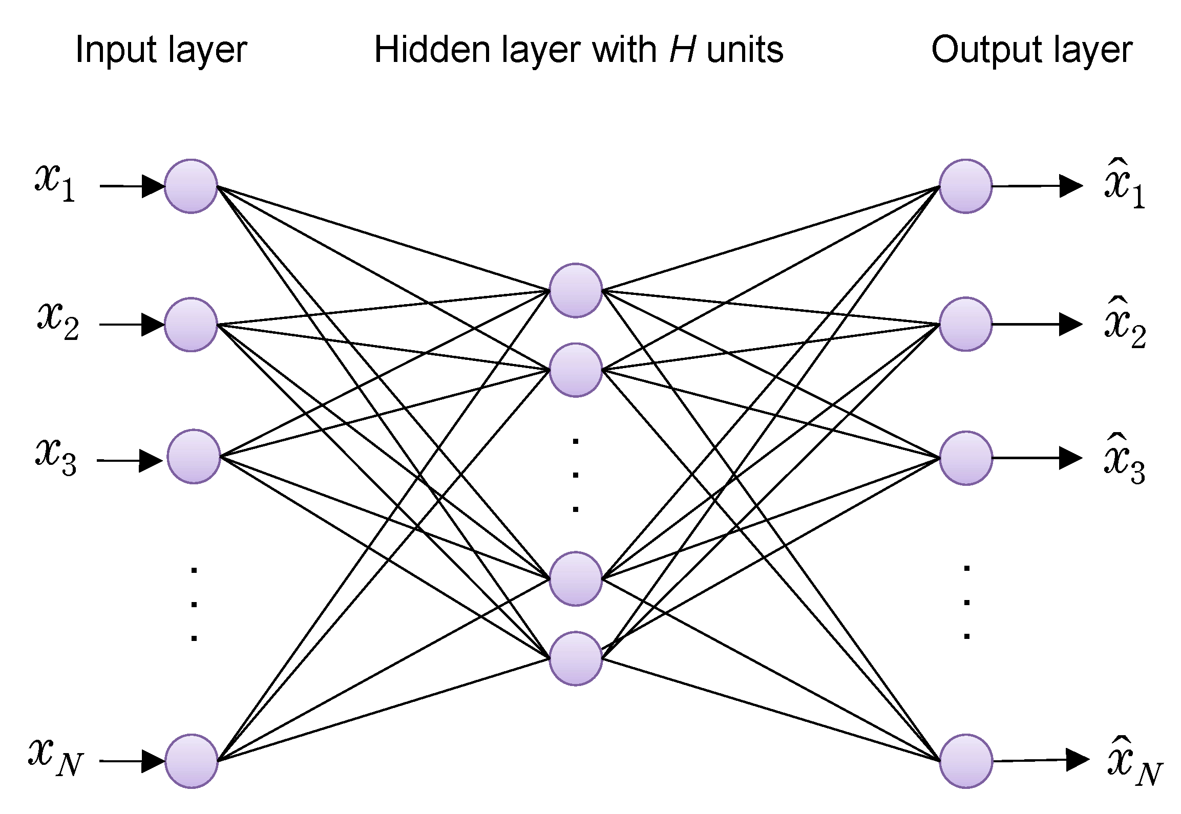
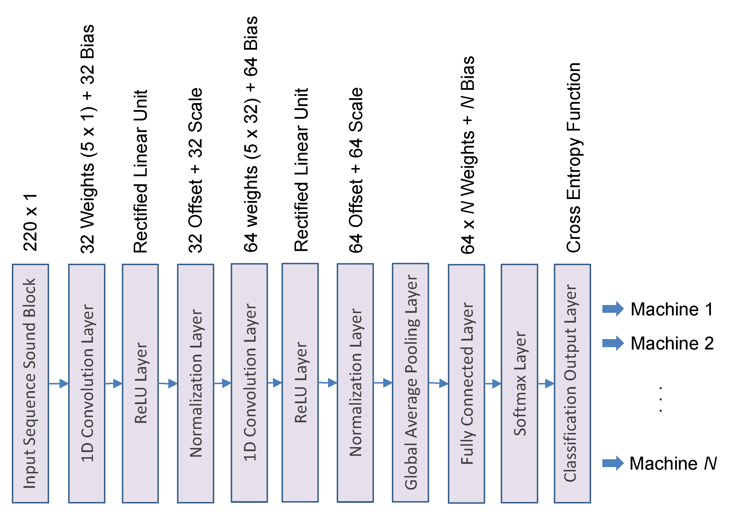
The main objective of this paper is to establish an identification system based on machine tools’ sounds without using conventional frequency domain information, but only raw time series data are used. As surveyed above, there seems to be almost no discussion about the optimal way to design time series sound data-based machine learning models. Also, it seems that concurrent visualization of understanding is not well realized when NN models are applied to anomaly detection of time series data such as mechanical sound data. In this paper, the authors have considered neural network systems that can be easily applied to classification, anomaly detection and prediction of CNC machine tools, as shown in Figure 3. In addition to images and videos used for training, in order that time series data such as mechanical sounds and vibrations can be used as multidimensional vector data, design functions for shallow NN, recurrent NN, 1D CNN, and AE are implemented in the application shown in Figure 2. For training machine learning models, many sound block (SB) data extracted with a designated sampling time are generated from nine categories of mechanical sounds collected from multiple machine tools. We report on the evaluation of the classification performance of each model on test data while changing the extraction time, which determines the length of the sound block, and the number of sound blocks used for training.

Figure 3. Example of machining scene of a large wood material using a long ball-end mill for a long time (SOLIC Co., Ltd., Ohmuta, Japan).

Finally, SB data-based FCDD is proposed for multi-dimensional vector data to realize anomaly detection of time-series data and its concurrent visualization of understanding, in which for example, time-series sound data are converted to one-line gray-scale images followed by BMP images for training FCDD. The effectiveness of the proposed model is evaluated by experiments.

2. Machining Tool Operating Sound and SoundBlocks

In the experiment, multiple machine tools installed at the university’s machine design and manufacturing center were operated, and nine categories of operating sounds were collected for 10 s each using a sampling rate of 44,100 [Hz]. No special sensor was used, but a microphone on a handheld smartphone was used. Recorded sounds were saved in each WAV file. When a smartphone’s microphone is used to measure SB data, problems such as picking up background noise and depending on placement may sometimes occur. In this experiment, the measurements were conducted by a microphone in hand just around the target machine tools so that such undesirable phenomena were not observed. However, if multiple machine tools are operating nearby, such problems should be noted.

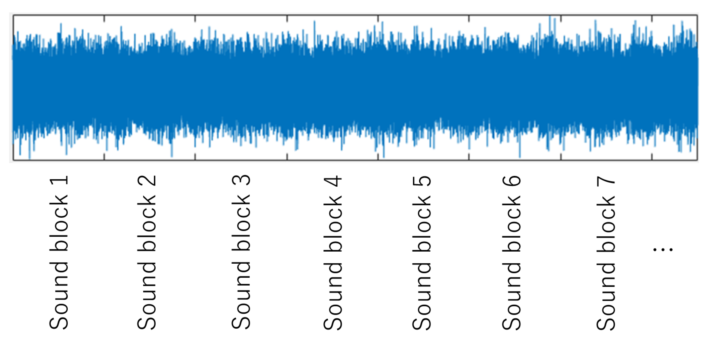
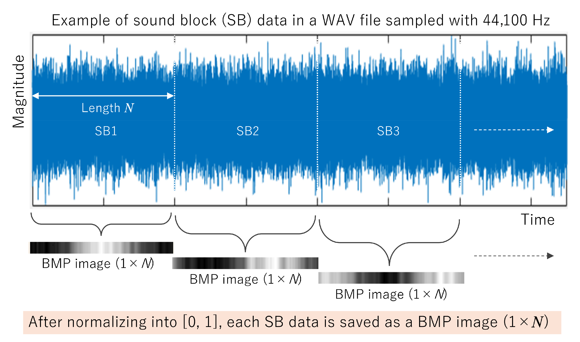
Sound blocks extracted from WAV files are used for training neural network models. Figure 4 shows an example of extraction of time-series sound block (SB) data from a WAV file, which is recorded from a general milling machine. In this experiment, SB data are sampled with 0.005 [s], so that the length of an SB data file is 44,100 × 0.005 = 220. According to the length, the number of input layer’s neurons is designed as 220. Also, in this case, the number of SB data extracted from a WAV file becomes 2000, whose 80%, 10%, and 10% are assigned for training, validation, and test, respectively. Details, including labels, are tabulated in Table 1. It has been empirically confirmed that it is important to determine the length of SB data used for training and testing. Note that the size of the dataset, the organization for training, validation and testing, and the length of one SB data were empirically determined in this case. It seems to be required to reconsider those values if conditions, including target materials, cutting tools, and machine tools, are changed.

Figure 4. Sound blocks extracted from a WAV file (.wav), which are used for training, evaluation, and test of NN models.

Table 1. Labels and number of sound blocks for training, validation and test.

Label	Training	Validation	Test
B13S_S600	1600	200	200
B13S_S1700	1600	200	200
TSL-360CNC_S500	1600	200	200
TSL-360CNC_1000	1600	200	200
TSL-360CNC_S1500	1600	200	200
TSL-360CNC_S2000	1600	200	200
Band Saw	1600	200	200
Milling-Machine	1600	200	200
Lathe	1600	200	200

3. Training and Evaluation of a Conventional Shallow Neural Network, 1D CNN, andAutoencoder

3.1. Neural Networks forClassification

Table 1 shows the numbers of sound blocks prepared for training, evaluation, and test of nine categories. It may seem that only 1600 samples for each class are too small for acquiring generalization by deep learning, and the results likely depend heavily on the specific train-test split. However, generally speaking for deep learning, if almost the same generalization ability is obtained, the smaller the dataset size is, the better the training process is. However, the authors plan to increase the amount of SB data to enhance the generalization ability if identification rates are not successfully obtained in future experiments.

Figure 5 and Figure 6 show four-layered normal neural networks and recurrent neural networks, respectively. The numbers of units in the first and second hidden layers are 100 and 50, respectively. Moreover, Figure 7 shows the structure of a 1D CNN consisting of 11 layers, in which the number N of labels from the output layer is 9 according to the classification task of nine categories.

Figure 5. Neural network whose input and output data are a sound block $x={[x_1,x_2,\cdots ,x_{220}]}^T$ and stochastic variable given by the Softmax function, respectively.

Figure 6. Recurrent type neural network whose input and output are the same as those in Figure 5.

Figure 7. One-dimensional CNN with the same input and output structure as Figure 5 and Figure 6.

After training the three models with the adaptive moment estimation (ADAM) [15] and cross entropy loss, they were compared and evaluated through a classification task of test SB data. As a result, mean values of classification accuracies are 87.6%, 88.4%, and 99.5%, respectively. Although there was no significant difference in classification performance between NN and RNN, higher classification performance was obtained with 1D CNN, as shown in Figure 7. As for training time, also, although the NN and RNN required approximately tens of thousands of epochs to converge, the 1D CNN was trained in a shorter time. Actually, the numbers of training weight parameters of NN, RNN, and 1D CNN were 27,609, 52,609, and 11,273, respectively. Table 2 shows each layer’s output activation and the numbers of parameters. Note that the meanings of T and C are time series data and the number of channels, respectively. It is expected from the above results that, in the future, anomaly detection using 1D CNN will be possible by redesigning the final output layer for binary classification, i.e., normal and anomaly, and by training it using normal and anomaly machining sounds accumulated in the target domain.

Table 2. Structural parameters of 1D CNN (T: time series data, C: channel).

Type	Activation	Parameters
Sequence Input	1(T)	-
1D Convolution	1(T) × 32(C)	Weights: 5 × 1 × 32, Bias: 1 × 32
ReLU	1(T) × 32(C)	-
Normalization	1(T) × 32(C)	Offset: 1 × 32, Scale: 1 × 32
1D Convolution	1(T) × 64(C)	Weights: 5 × 32 × 64, Bias: 1 × 64
ReLU	1(T) × 64(C)	-
Normalization	1(T) × 64(C)	Offset: 1 × 64, Scale:1 × 64
Glb. Avg. Pooling	1(T) × 64(C)	-
Fully Connected	9(C)	Weights: 9 × 64, Bias: 9 × 1
Softmax	9(C)	-

3.2. Autoencoder for AnomalyDetection

When the objective is to detect abnormalities in machine tools, etc., it seems effective to apply an autoencoder model that can be trained using only normal machining sounds. In this evaluation experiment, an autoencoder is designed as shown in Figure 8. A structural feature of the autoencoder is that the input and output layers have the same number N of units. The loss function is given by Equation (1), which is composed of the mean squared error (MSE) loss, the L2 regularization term of weights, and sparse regularization term based on Kullback–Leibler Divergence (KLD) [16]. The autoencoder is trained so that sound blocks at the input layer can be equivalently generated from the output layer. The autoencoder is trained such that every sound block $x\in {\Re }^{N\times 1}$ in the training data given to the input layer can be neuron-level-equally reconstructed as $\widehat{x}\in {\Re }^{N\times 1}$ at the output layer.

$$\begin{array}{c}\hspace{1em}\hspace{1em}\hspace{1em}\hspace{1em}\hspace{1em}\hspace{1em}E={\displaystyle \frac{1}{M}}{\displaystyle \frac{1}{N}}\sum _{m=1}^M\sum _{n=1}^N{\left(x_{mn}-{\widehat{x}}_{mn}\right)}^2\\ \hfill +\alpha \left[\sum _{i=1}^N\sum _{j=1}^H{\left(w_{ij}^1\right)}^2+\sum _{j=1}^H\sum _{k=1}^N{\left(w_{jk}^2\right)}^2\right]\\ \hfill +\beta \left[\sum _{i=1}^H\left\{\rho log{\displaystyle \frac{\rho }{{\widehat{\rho }}_i}}+(1-\rho )log{\displaystyle \frac{1-\rho }{1-{\widehat{\rho }}_i}}\right\}\right]\end{array}$$

(1)

where N is the length of a sound block, which is the number of units in both input and output layers. H and M are the numbers of units in the hidden layer and that of all the sound blocks in training data. $w_{ij}^1$ are the weights between the input layer and hidden layer, and $w_{jk}^2$ are those between the hidden layer and output layer. Also, $\alpha$ and $\beta$ are the coefficients to weight the degrees of penalties of L2 regularization and sparse regularization, respectively. Note that ${\widehat{\rho }}_i$ in the third term is the mean value of activation generated by the sigmoid function h at the ith unit in the hidden layer, which is given by

$$\begin{array}{c}\hfill {\widehat{\rho }}_i={\displaystyle \frac{1}{M}}\sum _{j=1}^{M}h\left({\mathit{w}}_i^{\left(1\right)T}{\mathit{x}}_j\right)\end{array}$$

(2)

where ${\mathit{w}}_i^{\left(1\right)T}$ is the ith row data in the weight matrix ${\mathit{w}}^{\left(1\right)}$, and ${\mathit{x}}_j$ is the jth training data. Note that $\rho$ in Equation (1) is the desired value of $\widehat{\rho }$, to which 0.05 is set. As can be seen, the loss function to train the autoencoder is composed of the first term about MSE, the second term about L2 regularization, and third term about sparse regularization based on KLD.

Figure 8. Autoencoder with N = 2205, whose input and output are a sound block vector $x={[x_1,x_2,\cdots ,x_{2205}]}^T$ and its reconstructed vector $\widehat{x}={[{\widehat{x}}_1,{\widehat{x}}_2,\cdots ,{\widehat{x}}_{2205}]}^T$, respectively.

In training the autoencoder, the reconstruction loss included in Equation (1) according to an input of sound block $x\in {\Re }^{N\times 1}$ is given by

$$\begin{array}{c}\hfill E_{\mathrm{m}\mathrm{s}\mathrm{e}}={\displaystyle \frac{1}{N}}\sum _{n=1}^N{\left(x_n-{\widehat{x}}_n\right)}^2\end{array}$$

(3)

A threshold value is defined as the maximum value of $E_{\mathrm{m}\mathrm{s}\mathrm{e}}$ obtained during the training. After training, if $E_{\mathrm{m}\mathrm{s}\mathrm{e}}$ obtained from an SB for the test is under the threshold value, then the SB is predicted as the same machine as the autoencoder; otherwise, it is a different machine. This means that if the autoencoder is trained using the SB data extracted from one machine tool, the test SB data can be predicted as the same machine or not.

In experiments, SB data of a band saw shown in Table 1 is used for training the AE. At the first step, the extracted time of a sound block is set to 0.005 [s], i.e., data length N is set to 220 (=44,100 × 0.005), however, a successful identification result could not be obtained. Accordingly, the extracted time is gradually increased to 0.05, i.e., N = 2205, so that each 300 test SB data except the band saw could be well identified as different from those of the band saw as shown in Table 3. Table 3 seems to be not a real anomaly detection result but a classification task. However, the AE tested in Table 3 was trained using only the SB data of the band saw, i.e., it is assumed that the SB data of the band saw and other machines are normal and not normal, respectively. It is suggested from the small MSE loss value of 0.00099 of the band saw that the trained AE is able to identify test SB data of a target machine from others.

Table 3. Max and mean values of MSE in giving nine kinds of test SB data to the trained AE. Note that the SB data of band saw was used to train the AE.

Label	MSE Loss (Max)	MSE Loss (Mean)	Number of Misclassified
B13S_S600	0.03324	0.02738	0/300
B13S_S1700	0.05668	0.02830	0/300
TSL-360CNC_S500	0.00431	0.00250	1/300
TSL-360CNC_1000	0.00562	0.00374	1/300
TSL-360CNC_S1500	0.00730	0.00482	1/300
TSL-360CNC_S2000	0.01077	0.00792	1/300
Band Saw	0.00121	0.00099	0/300
Milling-Machine	0.02555	0.02159	0/300
Lathe	0.01447	0.01068	0/300

Note that the number of neurons H in the hidden layers is 1000; consequently, that of all the weight parameters is 4,413,205. It is expected from the results that detection of anomalous mechanical sound will be possible by training the autoencoder based on the sound in a normal situation.

4. SB Data-Based FCDD Model for Anomaly Detection and Visualization of Time SeriesData

It has been confirmed from the experiments up to the previous sections that 1D CNN and autoencoder are effective for classification and identification of SB data, respectively. As can be expected, 1D CNN is also applied to anomaly detection tasks by redesigning the output layer for binary classification, i.e., normal and anomaly.

As for the data type processed by conventional anomaly detection systems, abnormality diagnosis systems, or fault diagnosis systems for CNC machine tools, original time-series sound data measured seem to need complicated transformation to the frequency domain to obtain, e.g., a spectrogram. For example, Jauregui et al. presented a methodology for the detection of tool wear based on frequency and time-frequency analysis of the cutting force and vibration signals [17]. Zhang et al. proposed a multi-modal fusion feature extraction method in which support vector machines, random forests, and deep NNs are employed to handle time-domain, frequency-domain, and joint time-frequency domain features, respectively, to build tool wear prediction models [18]. Also, Rahman et al. proposed vibration-based tool condition monitoring for the CNC grinding process, in which key features indicating tool wear and faults are extracted from the frequency domain using an image embedding technique [19]. On the other hand, our proposed SB data-based FCDD has only to directly deal with time-series data extracted from, e.g., cutting sound by a router bit. As for the network structure, for example, Kunitake et al. proposed an anomaly detection system using four models consisting of an SVM and three NNs for predicting machining troubles [20]. On the other hand, our proposed SB data-based FCDD can be simply designed based on pretrained powerful CNN models such as AlexNet and VGG19.

4.1. The Proposed FCDD for Time Series Data Such as SBData

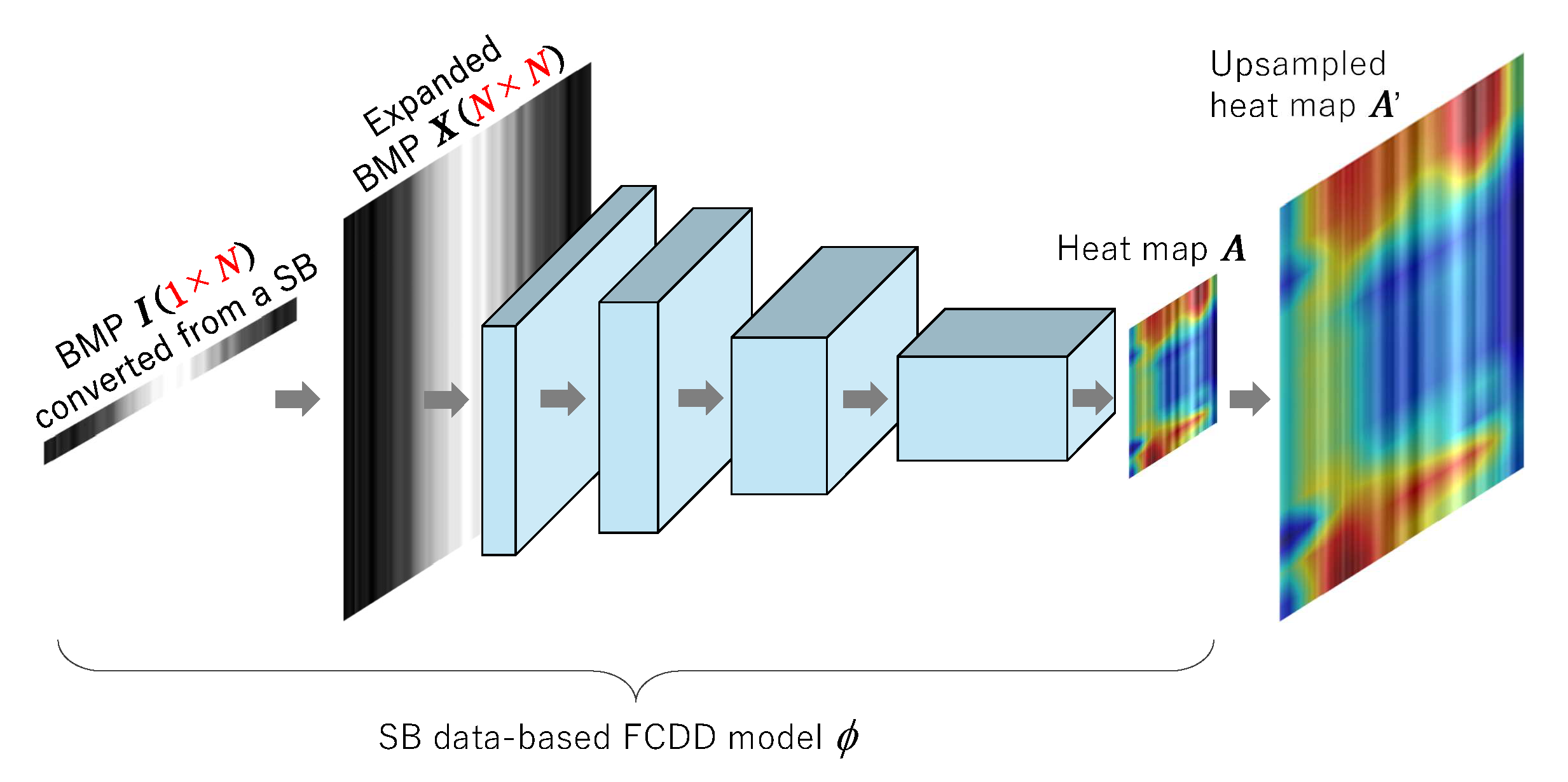
At this stage, one of the serious problems in dealing with the time series data such as SB data is how clearly and concurrently anomaly areas should be visualized and understood. In this paper, to cope with the need, an SB data-based FCDD model is further proposed as shown in Figure 9 to perform anomaly detection and its concurrent visualization without secondly using Grad-CAM [21] or Occlusion Sensitivity [22]. The FCDD model is designed based on VGG19, whose input layer’s resolution is $224\times 224$. The proposed method allows us to construct an FCDD-based anomaly detection system for time series data such as SB data.

Figure 9. Structure of our proposed SB data-based FCDD model for anomaly detection and its concurrent visualization, in which VGG19 with $224\times 224$ sized input layer is used for the backbone network.

The objective function of FCDD [23] is briefly introduced. In Liznerski’s paper, an FCN model ϕ employed in the former part performs ϕ: ℝ^c×h×w → ℝ^u×v, by which a feature map $\varphi (\mathit{X};\mathcal{W})$ downsized into $u\times v$ is generated from an input image X. A heat map of defective regions can be produced based on the feature map. The pseudo-Huber loss $\mathit{A}\left(\mathit{X}\right)$ [24] in terms of an output matrix from the FCN part, i.e., a feature map, is given by

$$\begin{array}{c}\hfill \mathit{A}\left(\mathit{X}\right)=\sqrt{\varphi {\left(\mathit{X};\mathcal{W}\right)}^2+1}-1\end{array}$$

(4)

where the calculation is performed with element-wise operation, i.e., pixel-wise, to be able to form a heat map. The object function in training an FCDD model is given by

$$\begin{array}{c}\hfill \underset{\mathcal{W}}{min}{\displaystyle \frac{1}{n}}\sum _{i=1}^n\left(1-y_i\right){\displaystyle \frac{1}{u·v}}{\parallel \mathit{A}\left({\mathit{X}}_i\right)\parallel }_1\\ \hfill -y_{i}log\left(1-exp\left(-{\displaystyle \frac{1}{u·v}}{\parallel \mathit{A}\left({\mathit{X}}_i\right)\parallel }_1\right)\right)\end{array}$$

(5)

The first term has a valid value in case that the label of a training image is negative, i.e., $y_i=0$, where the L1 norm $\parallel \mathit{A}\left({\mathit{X}}_i\right){\parallel }_1$ is divided by the total pixels $u·v$ of a feature map. The value can be considered as the average per one pixel. Therefore, when normal images are given to the network in training, the weights are adjusted so that each pixel forming a heat map can approach to 0.

On the other hand, the second term becomes effective when the label of a training image is an anomaly ($y_i=1$), and $exp(·)$ has a value close to 0 with the increase in the average loss per one pixel, so that the value of the log function $log(·)$ also approaches 0 with the lapse of training time. It is confirmed from the above discussion that Equation (5) using Equation (4) enables both to minimize the sum of the averages of $\parallel \mathit{A}\left({\mathit{X}}_i\right){\parallel }_1$ of non-defective images and to maximize those of defective images. The main dialog shown in Figure 1 enables the user-friendly training, testing, and building of FCDD models.

4.2. How to Generate Image Data from SBData

An FCDD model with the backbone consisting of VGG19 is tried to be applied to an identification task of machine tools’ sounds and their concurrent visualization, so that time-series SB data must be transformed into image maps with the same resolution as VGG19’s input layer. To cope with this indispensable process with the simplest method, SB data are simply copied into rows.

In this subsection, it is explained how to generate input images $\mathit{X}\in {\Re }^{N\times N}$ for FCDD from SB data in the time-series domain. As shown in Figure 9, X has the same resolution as the input layer of FCDD. As already explained, SB data $\mathit{s}\in {\Re }^{1\times N}$ is directly extracted from a WAV file with a designated extraction time $\Delta t$ [s]. For example, if the sampling frequency of a WAV file is f [Hz], then the length N of SB data becomes $f\Delta t$. One line of SB data $\mathit{s}=[s_1,s_2,\cdots ,s_N]$ is transformed to 1 line gray-scale BMP image $\mathit{I}=[I_1,I_2,\cdots ,I_N]$ as shown in Figure 10 through normalization by

$$\begin{array}{c}\hfill I_i={\displaystyle \frac{s_i-s_{\min }}{s_{\max }-s_{\min }}}(i=1,2,\cdots ,N)\end{array}$$

(6)

where $s_{\max }$ and $s_{\min }$ are the maximum and minimum values of elements in s, respectively. Then, an expanded bitmap image $\mathit{X}\in {\Re }^{N\times N}$ to be given to the input layer of FCDD can be constructed as

$$\begin{array}{c}\hfill \mathit{X}=\left[\begin{array}{c}\mathit{I}\\ \mathit{I}\\ ⋮\\ \mathit{I}\end{array}\right]\end{array}$$

(7)

Note that $N=224$ in the following experiments.

Figure 10. One line of BMP files generated from SB data for training an FCDD model.

4.3. Experiment of Identification of Machine Tools’ Sound Data and Its Concurrent Visualization Using an FCDDModel

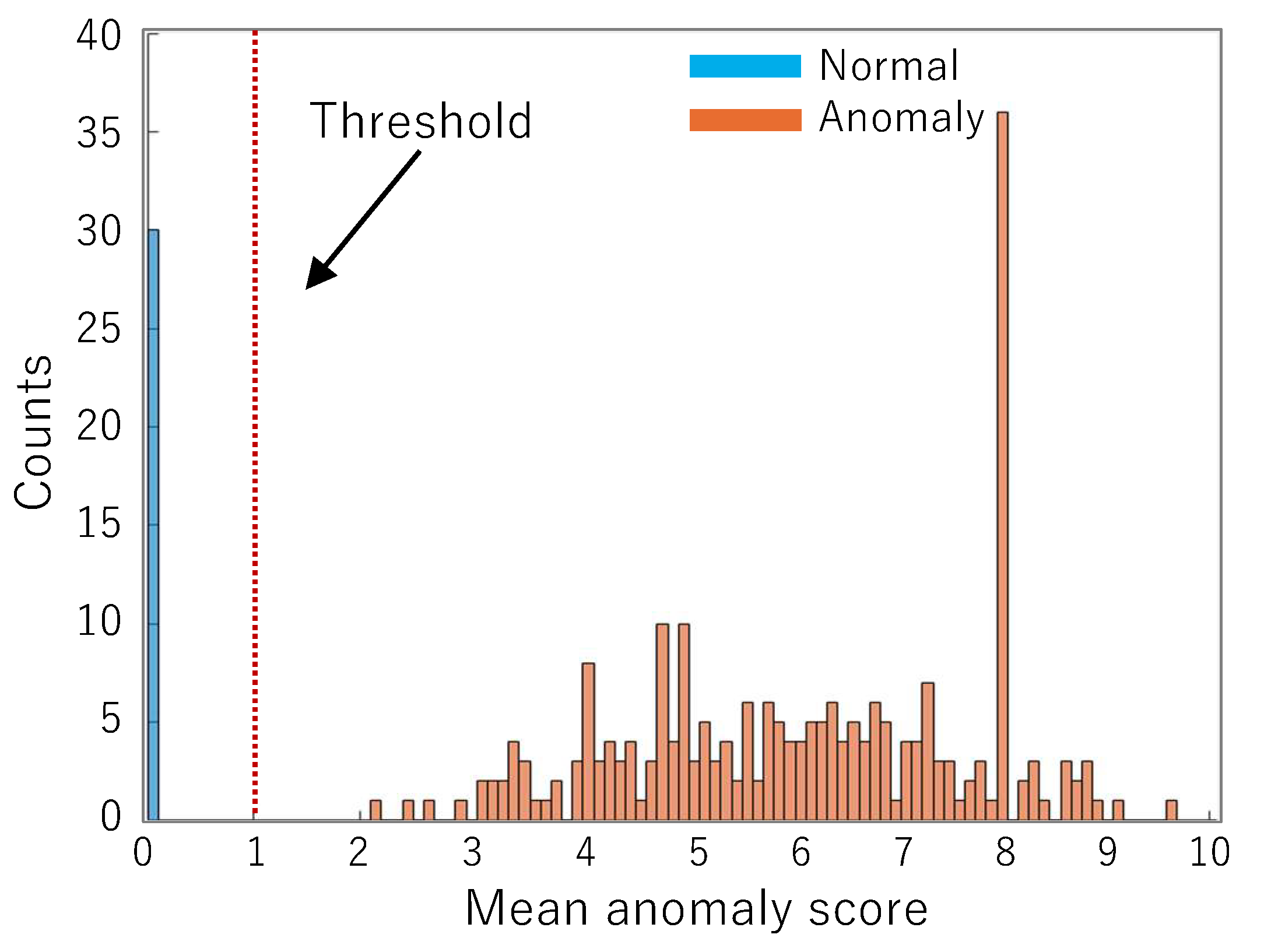
In this subsection, an identification experiment is conducted using the nine kinds of SB data as shown in Table 4, in which it is assumed that the sound of the band saw is normal and the other eight kinds of sounds are anomaly, so that 30 normal SBs and 30 × 8 = 240 anomalous SBs are used for training the FCDD model. After 200 epochs of training, all the training data were scored as shown in Figure 11. As can be seen, it is observed from the histogram given by Figure 11 that SB data extracted from band saw are scored with values close to 0; on the other hand, SB data except for band saw are scored with values far from 0. The mean anomaly score $Sc$ is calculated by

$$\begin{array}{c}\hfill Sc={\displaystyle \frac{1}{u·v}}{\parallel \mathit{A}\left({\mathit{X}}_i\right)\parallel }_1\end{array}$$

(8)

which is the mean value of each pixel in a predicted map $\mathit{A}\left({\mathit{X}}_i\right)$ given by Equation (4). In order to use the trained FCDD as an anomaly detector, a threshold value for criteria has to be set. In this case, a threshold value of 1 of the anomaly score can be easily determined from the distribution in Figure 11.

Table 4. Labels and number of sound blocks for the training and testing of an FCDD model.

Label	Machine Tool	Training	Test
Normal	Band Saw	30	300
Anomaly	B13S_S600	30	300
Anomaly	B13S_S1700	30	300
Anomaly	TSL-360CNC_S500	30	300
Anomaly	TSL-360CNC_1000	30	300
Anomaly	TSL-360CNC_S1500	30	300
Anomaly	TSL-360CNC_S2000	30	300
Anomaly	Milling-Machine	30	300
Anomaly	Lathe	30	300

Figure 11. Scores of training images evaluated by the trained FCDD model, i.e., training result.

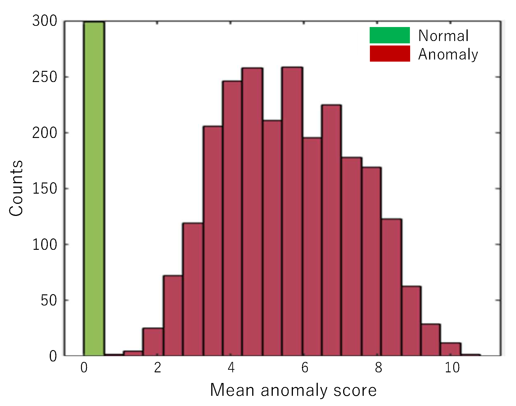
After setting 1 to the threshold value, the generalization ability of the trained FCDD was checked using test SB data. A total of 300 normal SBs and 300 × 8 = 2400 anomaly SBs were used for testing so that all the images could be accurately classified as normal (band saw) or anomaly (except for band saw) as shown in Table 5. Figure 12 shows the histogram of the test SB data’s mean anomaly scores predicted by the FCDD model. Incidentally, Figure 12 is the distribution of scores in which the trained FCDD predicted the test SB data for confirming the generalization. Although the distance between two class groups becomes smaller for test SB data, the test SB data could be successfully identified as shown in Table 5 by setting the threshold value to 1.

Table 5. Classification result of test SBs by the trained SB-based FCDD model (threshold = 1.0), in which it is assumed that the sound of a band saw is normal and other sounds are anomalies.

	Predicted	Anomaly (NG)	Normal (OK)
True
Anomaly (NG)		2400	0
Normal (OK)		0	300

Figure 12. Anomaly detection experiment using the trained FCDD model, in which it is assumed that the sound of a band saw is normal and other sounds are anomalies.

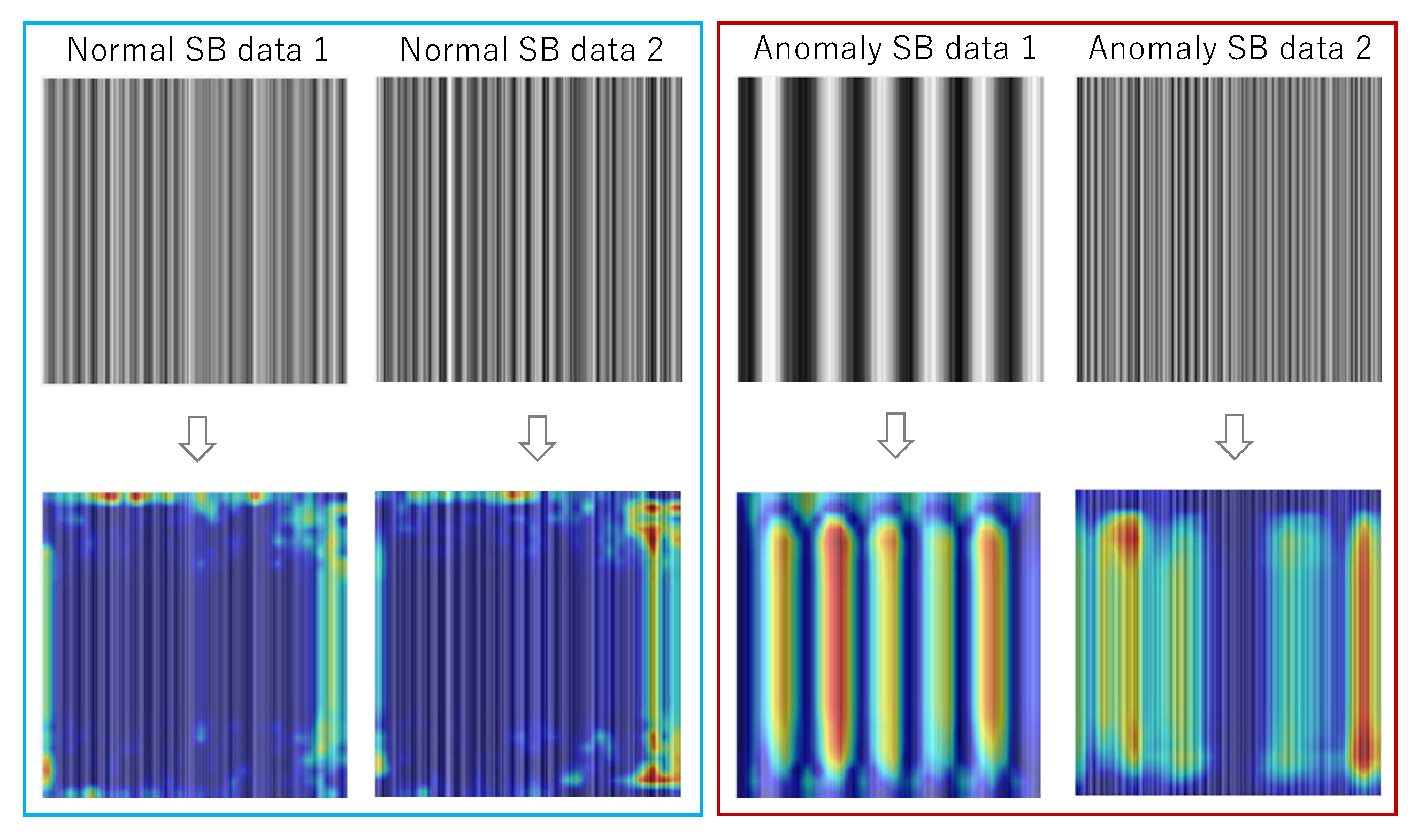
Figure 13 also shows examples of predicted maps generated by the FCDD, in which it is observed that anomaly regions within the time series data are validly visualized. Note that upper and lower figures are examples of inputs to and outputs from the trained FCDD model, respectively. The output from the FCDD model is a map with the same resolution as the input layer, so that heatmaps as shown in Figure 13 can be concurrently produced from the map without calling other visualizers such as Grad-CAM and Occlusion Sensitivity as a post-process. 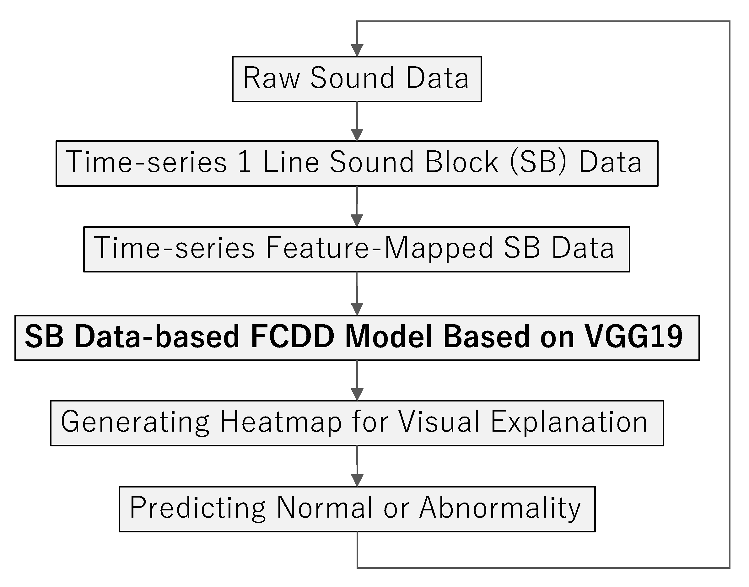Figure 14 shows the flow when the trained SB data-based FCDD model is applied to a real-time monitor of a CNC machine tool. Note that, in this experiment to test SB data tabulated in Table 4, one feature-mapped SB data for the input layer was concurrently visualized and predicted through one flow.

Figure 13. Examples of visualization results (heatmaps) of normal and anomaly sound areas generated by using the trained FCDD.

Figure 14. Flow of real-time monitor using trained SB data-based FCDD model.

It is known that smaller training datasets tend to lead to overfitting. However, if almost the same generalization performance is obtained, the smaller the dataset size, the better to reduce training time. It is observed from Table 5 that the FCDD model trained with only 30 samples per class can perform the promising generalization ability to 300 test samples per class. Naturally, for implementation in an actual machining process, it seems that the dataset needs more SB data with different sound features to enhance the generalization performance.

4.4. Discussions

As can be seen, the form of time-series SB data is not a map but multi-dimensional vectors, so that it cannot be directly given to the input layer of CNN models and CNN-based SVM models. Also, those models seem to not equip the function for concurrent visualization of understanding in predicting test images. As a post process, a visualizer such as Grad-CAM or Occlusion Sensitivity must be optionally called to make a heatmap, which shows the regions where CNN is interested in while classifying images. On the other hand, our proposed SB data-based FCDD model shown in Figure 9 can perform both prediction and visualization at the same time because the FCDD model can directly generate a heatmap.

The conversion to a 2D image by Equation (7) may seem to be redundant. However, the input layer’s resolution of FCDD depends on that of the CNN model used as the backbone network. The backbone network works as a feature extractor. The proposed SD-based FCDD model employs VGG19 for the backbone, so that the resolution of training and test images has to be fitted to that of VGG19. That is the reason why feature-mapped images for giving the FCDD are simply created by duplicating one line of SB data.

In the experiments introduced in this paper, the multi-class classification ability of SB data by NN, RNN, and 1D CNN, and the identification ability by AE are shown. Then, the binary-class classification ability of FCDD is evaluated. The binary-class classification task can be regarded as an anomaly detection task by setting two classes as normal and anomaly. It is suggested from the experiment results shown in Table 3 and Table 5 that the AE and FCDD models can be applied to anomaly detection tasks. As for 1D CNN, it is also possible to apply it to anomaly detection tasks by training it for binary classification using normal and anomaly SB data.

It is confirmed from Figure 11 that the FCDD model is well trained using the less training SB data shown in Table 1, in which it is assumed that SB data of the band saw and other machine tools are normal and abnormal, respectively. The valid threshold value for classification of test SB data can be easily determined by observing both distributions in Figure 11, e.g., by setting the center value between the maximum of normal scores and the minimum of anomaly ones. Judging from the results shown in Table 5, it seems that the classification of mapped test images in Table 1 was not particularly difficult. Because, in this evaluation, each machine tool’s WAV file that is the source of extracted SB data is a recording of relatively monotonous operating sound. However, it is observed from Figure 12 that the distance between two distributions of mean anomaly scores is close even for these test SB data, so that generalization to other test SB data that are extracted from different domains, e.g., such as different machine tools, materials, and machining conditions, may not be well performed. In the actual machining process, more complex operating sounds, including the sound of cutting material, are generated, so that additional training to enhance the generalization ability of the FCDD model is continuously required while increasing more training SB data with a variety of sound features of machine tools.

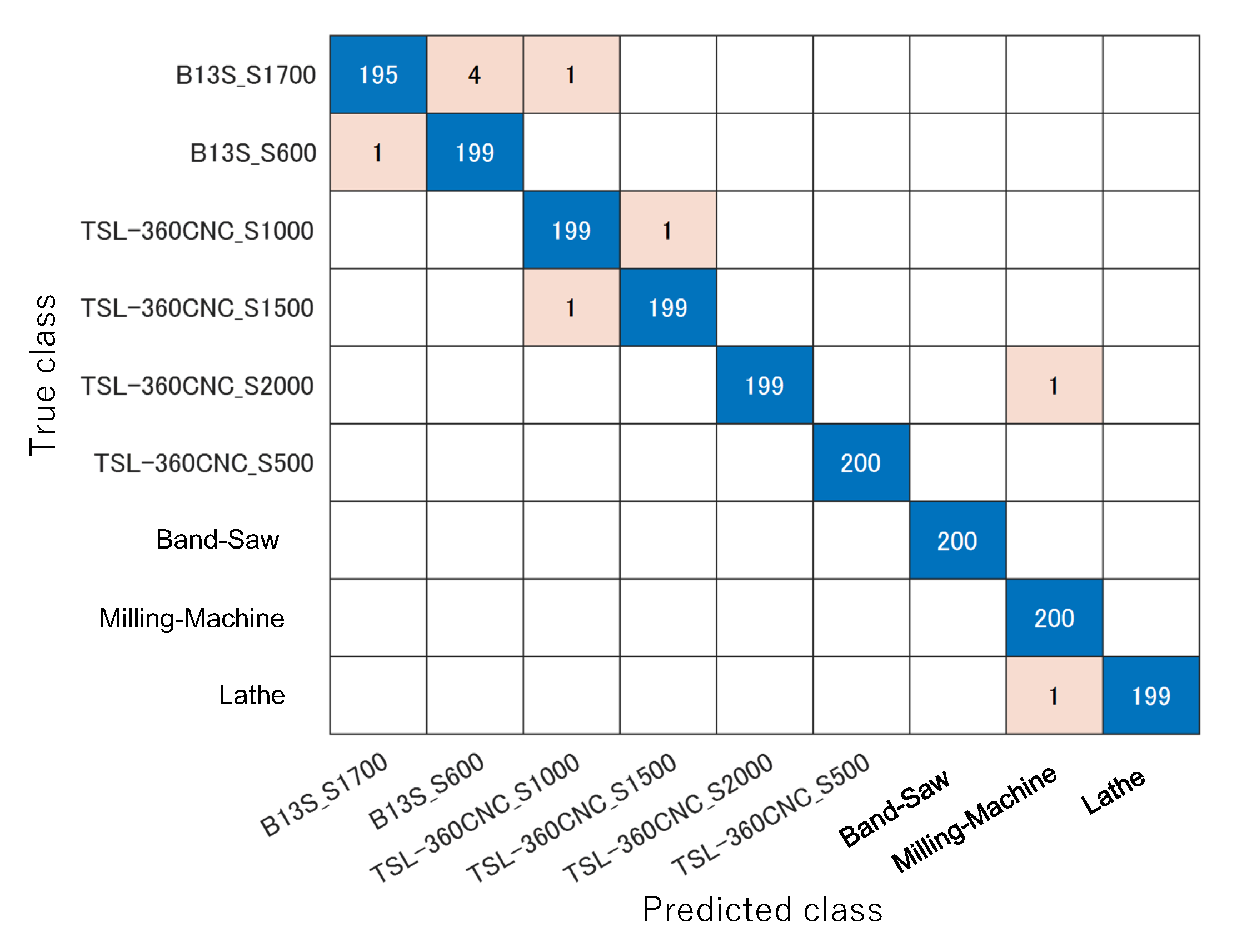
Compared with the above FCDD as an identifier, in Section 3.1, neural networks were applied to a classification task of nine kinds of SB data shown in Table 1 and were basically evaluated, in which the designed 1D CNN performed 99.5% classification result as shown in Figure 15, but some misclassifications were observed. It seems that continuous additional training is also necessary for 1D CNN to enhance its generalization ability. Also, as described at the end of Section 3.1, although 1D CNN can be used for binary classification, i.e., as an identifier or anomaly detector, post-processing such as Grad-CAM and Occlusion Sensitivity is additionally required for visualization of understanding.

Figure 15. Classification result of test SB data shown in Table 1 by the trained 1D CNN (confusion matrix).

5. Conclusions

The authors have been developing a design, training and building application with a user-friendly operation interface for CNN, CAE, SVM, YOLOX, SOLOv2, FCDD, and so on, which can be used for the defect detection of various kinds of industrial products even without deep skills and knowledge concerning information technology. In those models, images are basically used for training data. In this paper, an intelligent anomaly diagnosis system for CNC machine tools is considered, i.e., what structures of neural networks should be applied to the task. Mechanical sound and vibration generated from machine tools themselves or machining sound and vibration generated from router bits, i.e., end mill cutters, are recorded as wave files and used for training data. Extracted SB data from wave files are used for training NN models. It is confirmed from experiments that a 1D CNN and an autoencoder are effective for classification and identification of SB data, respectively. Then, an SB data-based FCDD model is further proposed for anomaly sound detection of removal machining by CNC machine tools and its concurrent visualization, in which time series data such as SB data can be directly applied to training and testing without converting them to other domains such as frequency. The effectiveness of the proposed method is shown through experiments.

In this paper, the dataset only consists of time-series SB data extracted from limited numbers of machine tools’ operating sounds. In future work, the proposed SB data-based FCDD model is planned to be applied to real-time monitoring of abnormality during endmill cutting by other CNC machine tools and their concurrent visualizations of understandings.