Applying Acoustic Scattering Layer Descriptors to Depict Mid-Trophic Pelagic Organisation: The Case of Atlantic African Large Marine Ecosystems Continental Shelf

Abstract

To identify key nonspecific organisational characteristics of the mid-trophic pelagic communities, which remain a challenge, we work with sound scattering layers (SSLs). Application was tested in the three African Atlantic Large Marine Ecosystems (AALMEs) to assess the utility of adapting and developing new acoustic variables. Our methodology allowed comparison between Large Marine Ecosystems (LMEs) based on 14 morphological, spatial and acoustic variables to characterize SSLs over time. These original variables were effective in monitoring and comparing the LMEs, and even allowed us to discriminate different organisations inside the Canary Current LME. Common traits identified for all AALMEs included the importance of the shallowest SSL. However, we identified an unexpected night-time pattern in SSL distributions in the Benguela Current LME which reflect a major difference in diel vertical migration mechanisms relative to other AALMEs. We also highlighted the predominance of elementary sampling unit (ESUs) with a single SSL and an unoccupied tiny layer close to the bottom, even if some ESUs presented up to six SSLs. Inter-annual changes in SSL organisation are highlighted by adaptation of original variables as the proportion of the water column occupied by SSLs and the relative importance of the shallowest SSL. SSL variables have been used mostly in deep water; here, we applied them on the continental shelf. SSL variables can be used to standardize the monitoring of marine ecosystems and capture change in spatial structure and function of mid-trophic pelagic marine ecosystems worldwide, even in data-poor areas where species identification of lower-trophic pelagic organism remains a challenge.

1. Introduction

Fisheries acoustics is effective for better understanding marine [1,2] and freshwater [3] ecosystems. Acoustic sensors are routinely used in scientific studies and monitoring programs [4,5,6]. For a long time, pelagic echo layers (or sound-scattering layers, SSLs) were considered as background noise when interpreting acoustics to study marine ecosystems [7]. Often, the acoustic reflections of fish schools had to be extracted or filtered from acoustic backscatter data to be analyzed properly [8,9].

Biological aggregations have been widely studied to understand what species aggregate, how and why aggregation form, and how we can study them [10]. There is a large variety of aggregations, from top predators to phytoplankton. In this study, we focus on SSLs, which can be produced by aggregations of a variety of pelagic species [11], such as aggregations of zooplankton [12,13], micronekton [14,15], gelatinous macronekton [16] and even phytoplankton [17,18,19]. These structures can be found in all oceans [20] and many studies address specific aspects of SSL, such as organisation and interactions [21] or their impact as biological pump [22]. Nonetheless, SSLs might react strongly to anthropogenic impacts and environmental fluctuations to create changes through SSL descriptors, mostly due to their short life cycle [23,24]. Some studies analyze SSLs to better understand a geographic area and their relationship with environmental data [25,26], with or without biological sampling. The early study of acoustic properties of SSLs started in the 1940s [20] and continue to today [27,28], especially with the use of narrow-band echo-sounding systems [29].

The present study takes advantage of previous studies and in particular on the work of Proud et al. [28], who worked on the standardization of metrics characterizing SSL. Our study advances and shows a new methodological approach to monitor Large Marine Ecosystems (LMEs) using SSLs without biological data. Diel Vertical Migration (DVM) is highly informational on vertical structuring and biocenoses function [26,28,30]. We used DVM in parts of the three African Atlantic Large Marine Ecosystems (AA LMEs) to demonstrate their utility to discriminate changes within an LME as well as differences and similarities between LMEs. We expect to observe DVM of type I [31] in the studied areas.

The aim of this study is to show the utility of our methodology based on SSLs in its ability to monitor and compare AA LMEs in the context of data-poor areas. The application on AA LME allows illustration of the efficiency of the method on a large dataset. Previous studies on these areas provided the ecological context [32,33,34,35,36,37,38]. We expect to observe differences within and between AA LMEs [33] applying our methodology. Interannual changes occur [35,39,40], so we can expect reported SSL changes over years. We compare SSL signals from AA LMEs to determine which variables might be useful for monitoring temporal change. To do this, we identified innovative SSL variables to describe SSL organization over the continental shelf of AA LMEs by first exploring spatial features using a dataset from several sea surveys carried out using the same research vessel and methods. Then, we analyzed the following: (i) temporal variability of SSL organization relative to short, diel-scale processes, i.e., to record DVMs of plankton, [41,42] and then (ii) document SSL’s inter-annual variation.

2. Materials and Methods

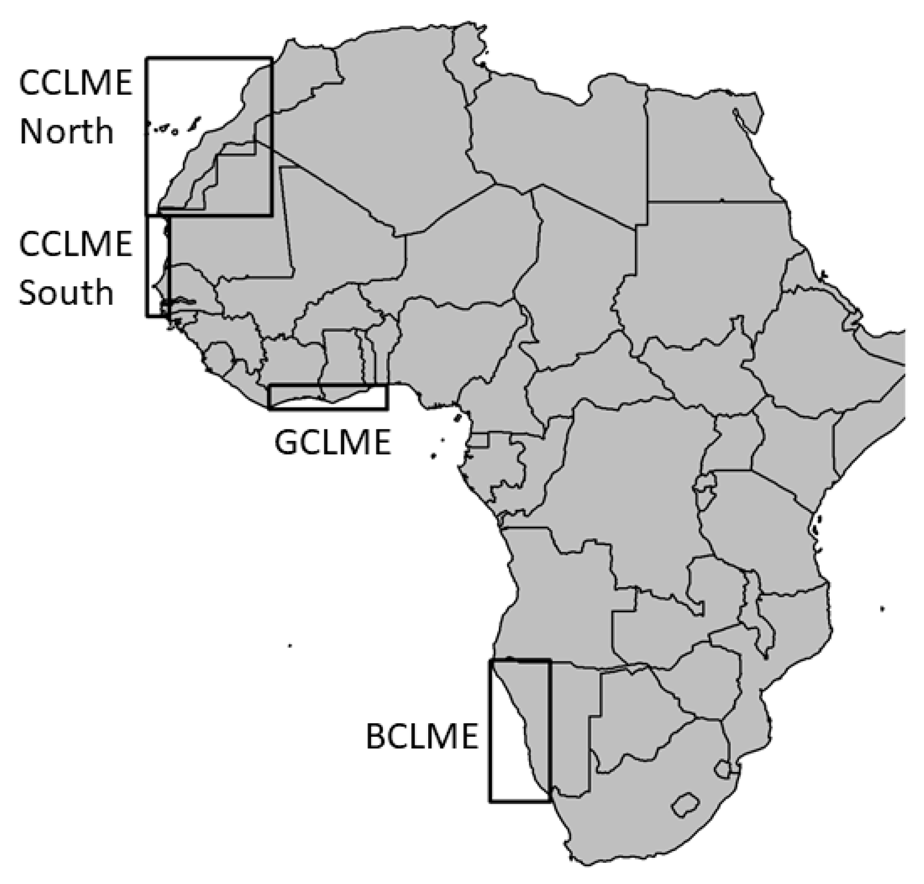
2.1. Material: Annual Acoustics Survey in African Atlantic Large Marine Ecosystems

Acoustic data were recorded using a 38 kHz echosounder [2] from 10 to 500 m depth on board the RV Dr Fridtjof Nansen. We used an ES38-B transceiver, hull mounted at a depth of 5.5 m, with an absorption coefficient of 8.7 dB km⁻¹, a pulse length of 1.024 ms and a maximum used transmission power of 2000 watts [43]. The echosounder was calibrated following classic calibration procedures [44]. Several authors have shown that the acoustic density measured at 38 kHz is a good indicator of micronektonic abundance [45,46,47]; this frequency is currently used in fisheries acoustic studies. SSLs have already been usually studied in deeper sea, e.g., [48,49,50]. In this study, we consider data on the continental shelf, i.e., with a depth under 150 m, to monitor changes in areas less studied than the high sea.

We recorded data over the continental shelf of the AA LMEs (Figure 1): the Canary Current Large Marine Ecosystem (CCLME), the Guinea Current Large Marine Ecosystem (GCLME) and the Benguela Current Large Marine Ecosystem (BCLME) [51] (Figure 1,

Table 1. Characteristics of acoustic surveys conducted in three African Atlantic Large Marine Ecosystems (LMEs). Annual surveys conducted in the Canary Current LME (n = 14) occurred in 1994–2006, 2011, 2015, in the Guinea Current LME (n = 8) in 1999-2006 and in the Benguela Current LME (n = 8) in 1994–2001. Transect lengths for each LME represent the total linear distance of all surveys conducted within the same LME; the Elementary Sampling Unit (ESU) is set at 0.1 nmi in length (during the same season and at depth < 150 m).

LME	Geographic Position	Sampled Years	Transect (nmi)	Number of Analysed ESU
Canary Current	34° N; 7° W to 12° N; 17° W	1994–2006, 2011, 2015	96,788	588,459
Canary Current North	20.8° N; 7.2° W to 34.1° N; 17.7° W	1994–2006, 2011, 2015	58,965	368,782
Canary Current South	12.2° N; 16.1° W to 20.8° N; 17.7° W	1994–2006, 2011, 2015	37,822	219,677
Guinea Current	4° N; 8° W to 6° N; 3° E	1999–2006	12,908	86,841
Benguela Current	17° S; 9° E to 31° S; 17° E	1994–2001	39,368	1086

). The CCLME extended from the Strait of Gibraltar (36° N, 5° W) to south of Guinea-Bissau (11° N, 16° W), with our study area encompassing coastal waters from 34° N, 7° W to 12° N, 17° W. This area was sub-divided into two ecologically distinct regions for sampling and analyses: North and South of Cape Blanc [52]. The area north of Cape Blanc exhibited continuous upwelling, while upwelling in the area to the south was seasonal [53]. We used data from 14 surveys in the CCLME from 1995 to 2015 totalling 99,788 nmi.

The GCLME extended from Bissagos Island (Guinea Bissau) in the north (11° N, 16° W) to Cape Lopez (Gabon) in the south (0° S, 8° E) [36]; our study area encompassed coastal waters from 4° N, 8° W to 6° N, 3° E. The dataset from the GCLME consisted of eight surveys from 1999 to 2006, totalling 12,908 nmi.

The BCLME occurs along the coast of south western Africa, stretching from the border between Namibia and Angola in the north (17° S, 11° W) southwards to the east of the Cape of Good Hope (South Africa) (29° S, 17° E) [37]. Our study area encompassed the coastal waters from 17° S, 9° E to 31° S, 17° E. Eight surveys were conducted in the BCLME from 1994 to 2001, totalling 39,368 nmi.

All survey designs were similar over years. Finally, we consider four marine ecosystems: CCLME North, CCLME South, GCLME and BCLME. A seasonal upwelling is present in both the southern Canary Current LME and the Guinea Current LME [34,54,55,56], whereas the upwelling in the northern Canary Current LME and the Benguela Current LME occurs year-round [53]. We used data from surveys not carried out during the seasonal upwelling.

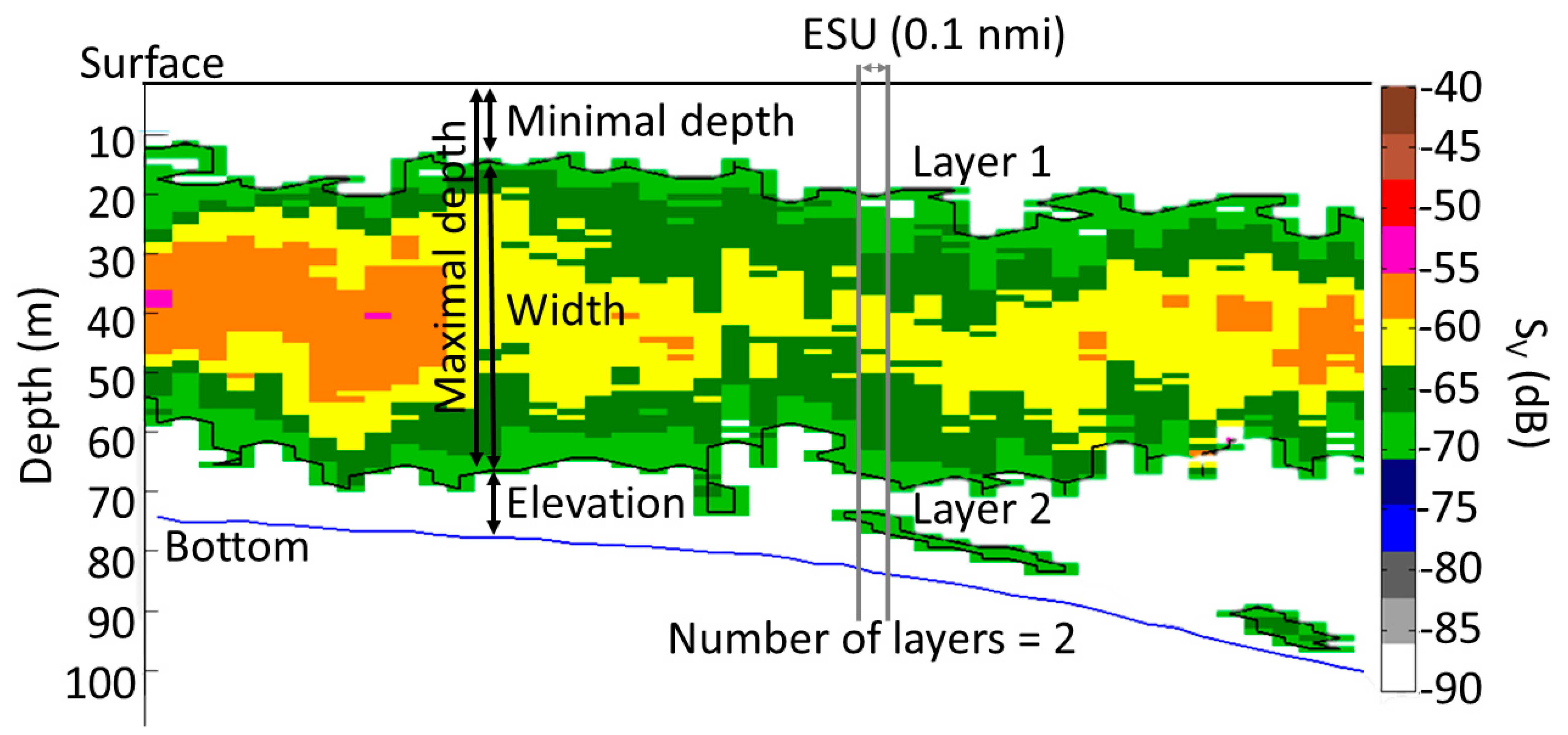
2.2. Methods: Fisheries Acoustics and Sound Scattering Layers

Acoustic data were converted and cleaned using Matecho [57]. We used the echo-integrated data at a spatial resolution of 0.1 nmi by 1 m depth. To extract SSLs, we post-processed data with a segmentation algorithm within Matecho at an echo level threshold of −70 dB re 1 m⁻¹ (noted dB from here). To characterize the SSLs in the water column, we computed SSLs variables for each elementary sampling unit (ESU) of 0.1 nmi length. We used the −70 dB value as the lower threshold defining micronektonic SSLs [31,58]. Because there was no upper threshold, SSLs included zooplankton, micronekton and all other pelagic organisms. To assess SSL spatial pattern variability at the inter-annual level, we used mean volume backscattering strength (S_v in dB) [6] as a proxy for relative pelagic abundance [58]. Before data analysis, we removed data related to transition periods in diel vertical migration patterns. Transition periods (dawn and dusk) were linked to sun azimuth data, i.e., by sun elevation, determined by data date, hour and geospatial position [59]. Hereafter, data from northern CCLME, southern CCLME, GCLME and BCLME were studied independently and named here after the respective marine ecosystems. Therefore, there are three LMEs and four marine ecosystems used in this study. We assumed that spatial auto-correlation in data along transects was negligible [14,60,61].

We used Matecho to compute six variables per ESU “j” for each SSL “i” (Figure 2): minimal depth (đ_i,j) [62], maximal depth (Đ_i,j) [62], width (Ẇ_i,j) [28,62], S_v (S_v,i,j) [6], s_A (s_A,i,j) [6] and the number of SSLs (Ŋ_j) [30,62,63]. We focused on variables related to the shallowest SSL (i.e., SSL_1,j), and all SSLs, from the shallowest to the deepest (SSL_all,j). We choose to focus on the shallowest SSL because they to have a major importance in our marine ecosystems, according to expert experience. Presented variables come directly from Matecho, i.e., đ_1,j, Đ_1,j, Ẇ_i,j, S_v,1,j, s_A,1,j, and we calculated đ_all,j, Đ_all,j, Ẇ_all,j, S_v,all,j, s_A,all,j.

From this set of variables, we inferred new variables: the elevation of the shallowest SSL (Å_1,j) and all SSLs (Å_all,j) [62]; the proportion of water column occupied by the shallowest SSL (Ṗ_1,j) and by all SSLs (Ṗ_all,j); and the relative importance of the shallowest SSL compared to all SSLs (Ċ_1,j). All calculations are detailed in

Table 2. List of all sound scattering layer (SSL) variables, symbol, unit and formulae. Sv is the volume backscattering coefficient in dB, sA is the area backscattering coefficient (m² nmi⁻²) [6]. N/A means category is not applicable. The term “i” is the SSL number, starting at 1 for the shallowest SSL and called “all” when including all SSLs. The term “j” is the ESU number.

Calculated Variable	Symbol	Unit	Formula	Reference(s)
Bottom depth at ESU j	Dj	m	N/A	-
Number of SSL at ESU j	Ŋj	-	N/A	[30,62,63]
Minimum depth of all SSLs at ESU j	đall,j	m	N/A	[62,64]
Maximum depth of the shallowest SSL at ESU j	Đ1,j	m	N/A	Adapted from [62,64]
Maximum depth of all SSLs at ESU j	Đall,j	m	${\displaystyle {\displaystyle \sum }_{i=1}^{\mathrm{Ŋ}}}{\mathrm{Đ}}_i$	Adapted from [62]
Minimal elevation of the shallowest SSL at ESU j	Å1,j	m	$D_j-{\mathrm{Đ}}_{i,j}$	Adapted from [62,65]
Minimal elevation of all SSLs at ESU j	Åall,j	m	$D_j-{\mathrm{Đ}}_{all,j}$	Adapted from [62,65]
Width of shallowest SSL at ESU j	Ẇ1,j	m	${\mathrm{Đ}}_{i,j}-{\text{đ}}_{i,j}$	[28,62]
Sv of shallowest SSL at ESU j	Sv, 1,j	dB re 1 m−1	$10 {\log }_{10}{s}_v$	Adapted from [6]
Mean Sv of all SSLs at ESU j	Sv, all,j	dB re 1 m−1	$10{\log }_{10}\frac{{\sum }_{i=1}^{\mathrm{Ŋ}}{10}^{\raisebox{1ex}{$S_{v,i,j}$}\!\left/ \!\raisebox{-1ex}{$10$}\right.}}{\mathrm{Ŋ}}$	Adapted from [6]
sA of shallowest SSL at ESU j	sA, 1,j	m2 nmi−2	$4 \pi \left(1852\right)²s_a$	Adapted from [6]
Mean sA of all SSLs at ESU j	sA, all,j	m2 nmi−2	$\frac{{\sum }_{i=1}^{\mathrm{Ŋ}}{s}_{A,i,j}}{N}$	Adapted from [6]
Proportion of the water column occupied by the shallowest SSL at ESU j	Ṗ1,j	%	$\frac{{\mathrm{Ẇ}}_j}{D_j}$	Present study
Proportion of the water column occupied by all SSLs at ESU j	Ṗall,j	%	${\displaystyle {\displaystyle \sum }_{i=1}^n}{\mathrm{Ṗ}}_{i,j}$	Adapted from [30]
Contribution of the shallowest SSL in the proportion of the water column occupied at ESU j	Ċ1,j	-	$\frac{{\mathrm{Ṗ}}_{i,j}}{{\mathrm{Ṗ}}_{all,j}}$	Present study

. In total, we worked with 14 variables.

We used the same SSL variable set for all AA LMEs, allowing us to compare ecosystems and analyse their diel migrations and inter-annual variabilities. Two of the SSL variables (number of SSLs and proportion of the water column occupied) that we used had already been used by [30,63,66], whereas two others (proportion of the water column occupied by the shallowest SSL and contribution of shallowest SSL in the proportion of the water column occupied) are new ones. The mixed layers, minimum oxygen and euphotic zone depths should influence both variables involved in calculating proportional occupancy of the water column. Other variables used have traditionally characterized acoustic pelagic fish school using, e.g., “shoal echo-integration” [62] and adapted here to SSL.

We calculated all statistics using R version 3.4.3 [67]. We used boxplots to compare medians and data distributions of continuous variables associated with the four marine ecosystems. We used ANOVA and the Wilcoxon test to compare non-parametric distributions of data between paired LMEs. For the comparison of more than two LMEs, we tested the marine ecosystems by pair. Differences were considered significant if the probability (p-value) of the statistical test was < 0.05. We used kernel density estimates [68] to scrutinize differences in distributions identified by the Wilcoxon tests. The resolution of each variable was used to define bandwidth parameters in the kernel density function. For discrete variables, we drew barplots and applied Chi-square tests (p-value < 0.05) to examine the extent of independence between variables [69].

To analyse differences between day and night in the four marine ecosystems, we drew two boxplots for each variable, one for daylight conditions and one for night-time conditions. A Wilcoxon test was used to compare means between day and night for each ecosystem and each variable. For discrete variables, we used the Chi-square test (p-value < 0.05) to compare values between day and night. To estimate inter-annual change, we applied a linear regression (p-value < 0.05) incorporating the mean value for each variable for each year. Polynomial regressions were also tested up to order 3.

A principal component analysis (PCA) was run to summarise multi-dimensional information and identify correlations between variables. The package “FactoMineR” [70] was used to run the PCA with standardized data.

Results are organised to present (i) the spatial variability between marine ecosystems, (ii) differences in diel vertical migrations organisations and (iii) changes over years.

3. Results

3.1. Spatial Variability of Sound Scattering Layers

When we compared the northern and southern areas of CCLME, we found that measurements of the variables for these two marine ecosystems differed significantly from one another (Supplementary Material S1). At a larger scale, i.e., among all AA LMEs, we found that 83 ANOVA tests were significant among 84 and, which indicates that variables were significantly different from one another according to Wilcoxon test results (see Supplementary Material S1 for descriptors not presented here), except s_A, _all between CCLME North and GCLME.

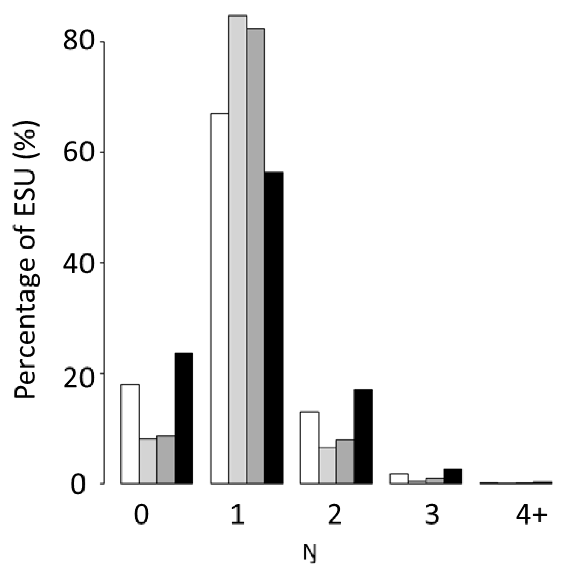
3.1.1. Number of Sound Scattering Layers (Ŋ) in the Water Column

The number of SSLs per ESU (Ŋ) differed significantly among marine ecosystems (Figure 3). CCLME south and GCLME had the highest number of ESUs (Ŋ) within a single SSL (more than 80%), whereas CCLME north and BCLME had the highest number of ESUs with either no SSLs (Ŋ = 0) or more than one SSL (Ŋ > 1). However, CCLME north and BCLME did not have the same mean number of SSLs. BCLME had more ESUs without any SSLs (Ŋ = 0) than any other marine ecosystem, but it also had the lowest proportion of ESUs with a single SSL (Ŋ = 1).

The analyses highlighted that ESUs with Ŋ = 1 are the majority whatever the marine ecosystems considered. In all marine ecosystems studied, Ŋ ≤ 6. Six layers (Ŋ = 6) where found in 90 ESUs, usually in waters of 100–140 m bottom depth.

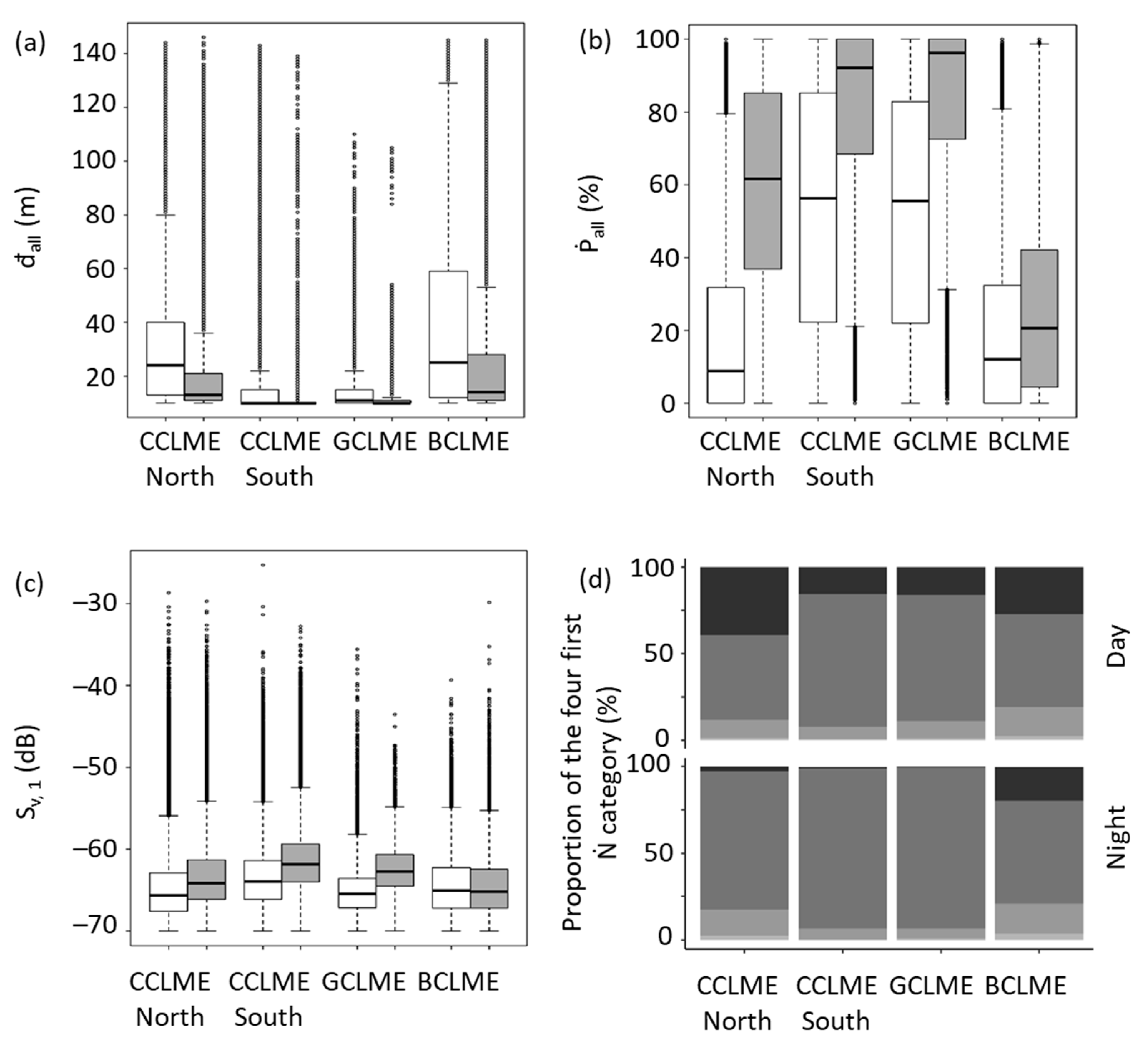
3.1.2. Minimum Depth of All SSLs (đ_all)

Minimum depths of all SSLs (đ_all) differed significantly among marine ecosystems (Figure 4a). Boxplots showed a strong difference in đ_all between the northern and southern CCLME marine ecosystems (Figure 4). The northern part of CCLME presented more important values of median and standard error (15 ± 16 m) for this variable than did the southern part (10 ± 7 m). However, density peaks of minimal depth of SSLs of the marine ecosystems occurred at similar depths (Figure 4b). Only size of the peak differed. Boxplots and density curves for the BCLME were similar to those of the northern CCLME, whereas data for GCLME were similar to the southern CCLME. The data showed that the four marine ecosystems conformed to two basic types: one type with a distinctive, high-density peak (CCLME south and CGLME), and a second type with a lower, less distinct density peak (CCLME north and BCLME).

3.1.3. Proportion of Water Column Occupied (Ṗ_all)

The proportion (in volume) of the water column occupied by all SSLs (Ṗ_all) differed significantly among marine ecosystems; boxplots highlighted variations for these differences (Figure 5a). Density curves for SSLs were bimodal and the peak density values differed between the northern and southern CCLMEs (Figure 5b). The highest peak (on the right side of Figure 5b, for Ṗ_all close to 100%), showed that for most ESUs (except in BCLME), the water column was filled more than 90% by SSLs. CCLME north and the BCLME were similar to each other and much different from the other two marine ecosystems relative to the proportion of the water column (by volume) occupied by SSLs. Indeed, only BCLME (and northern CCLME to a lesser extent) showed a density peak representing a sparsely filled water column (Ṗ_all close to 0–10%).

3.1.4. Mean Volume Backscattering Strength of First Sound Scattering Layer (S_{v, 1})

S_{v, 1} differed significantly among studied marine ecosystems (Figure 6a). Density curves of all marine ecosystems showed similar shapes, but they peaked at slightly different values (about −65.0/−60.0 dB). The peak backscattering strength for CCLME north was a bit lower than for CCLME south. The peak for CCLME north, at −65.6 dB, is close to the peak for BCLME (−66.6 dB), whereas the peak of CCLME south (−63.5 dB,) is similar to the peak for GCLME (−64.0 dB). However, mean S_{v, 1} values are quite similar among marine ecosystems.

3.2. Comparative Analysis of Diel Differences among Marine Ecosystems

All pelagic marine ecosystems in this study differed in their SSL spatial organisation over a diel cycle. All variables measured among marine ecosystems during daytime and night-time differed significantly (Figure 7), except for the maximum depth of the shallowest SSL (Đ₁) in BCLME (other variables, whose Đ₁, are shown in Supplementary Material S2 as statistical tests).

In all four marine ecosystems, đ_all (minimum depth of all SSLs) was deeper during the day than at night and included a more extensive range of depths (Figure 8a). The water column was also more filled with organisms at night than during the day. S_{v, 1} (mean volume backscattering strength of the shallowest SSL) was higher at night, except for water mass BCLME, where S_{v, 1} was similar during day and night. The number of ESUs (Ŋ) without SSLs was lower for all ecosystems at night. In CCLME north and BCLME, the proportion of ESUs with four SSLs or more was higher at night.

3.3. Inter-Annual Variability and Trends in the Atlantic African Large Marine Ecosystems

Testing variables to detect annual changes (1995–2015) in each marine ecosystems independently (Figure 8,

Table 3. Summary of the significance tests of the linear regression for change over time (y) for sound-scattering layer (SSL) variables collected from African Atlantic Large Marine Ecosystems. “NS” represents a non-significant p-values > 0.05. In each cell, the order of the polynomial regression and the adjusted R-squared (R²) are written, followed by the associated p-value in brackets.

Sound-Scattering Layers Variables (SSL)	CCLME		GCLME	BCLME
	North	South
Minimum depth of all SSLs (đall)	R2 = 7.45 × 10−3 (p < 2.2 × 10−16)	R2 = 4.56 × 10−3 (p < 2.2 × 10−16)	NS	NS
Maximum depth of first SSL (Đ1)	R2 = 3.46 × 10−3 (p < 2.2 × 10−16)	NS	NS	NS
Width of first SSL (Ẇ1)	R2 = 1.35 × 10−2 (p < 2.2 × 10−16)	NS	NS	NS
Minimum elevation of first SSL (Å1)	NS	R2 = 7.19 × 10−3 (p < 2.2 × 10−16)	NS	NS
Minimum elevation of all SSLs (Åall)	NS	R2 = 5.11 × 10−3 (p < 2.2 × 10−16)	NS	NS
Mean volume backscattering strength of first SSL (Sv, 1)	NS	NS	R2 = 2.71 × 10−2 (p < 2.2 × 10−16)	NS
Mean volume backscattering strength of all SSLs (Sv, all)	R2 = 4.73 × 10−3 (p = 0.090)	NS	R2 = 2.76 × 10−2 (p < 2.2 × 10−16)	NS
Nautical area scattering strength of first SSL (sA, 1)	NS	NS	NS	NS
Mean nautical area scattering strength of all SSLs (sA, all)	NS	NS	NS	NS
Proportion of the water column occupied by first SSL (Ṗ1)	R2 = 4.60 × 10−2 (p < 2.2 × 10−16)	NS	R2 = 2.37 × 10−2 (p < 2.2 × 10−16)	R2 = 6.64 × 10−2 (p < 2.2 × 10−16)
Proportion of the water column occupied by all SSLs (Ṗall)	R2 = 4.45 × 10−2 (p < 2.2 × 10−16)	R2 = 4.22 × 10−3 (p = 0.084)	R2 = 1.81 × 10−2 (p < 2.2 × 10−16)	R2 = 7.18 × 10−2 (p < 2.2 × 10−16)
Contribution of first SSL in the proportion of the water column occupied by (Ċ1)	R2 = 8.43 × 10−3 (p < 2.2 × 10−16)	NS	R2 = 3.80 × 10−3 (p < 2.2 × 10−16)	NS
Number of SSLs (Ŋ)	R2 = 2.55 × 10−3 (p = 4.83 × 10−3)	R2 = 2.37 × 10−3 (p = 0.0242)	NS	NS

), we found few SSL variables significantly responding. We report two types of inter-annual variations: without or with trend over years.

For the northern CCLME, the mean volume backscattering strength of all SSLs (S_{v, all}) and the number of SSLs (Ŋ) were the only two variables which decreased and increased, respectively, over the years (Figure 8c,i). The same variable (Ŋ) significantly increased over years in the southern CCLME (Figure 8j). In the southern CCLME, there was a significant increase in the proportion of the water column occupied by all SSL (Ṗ_all). The GCLME possessed three variables that showed significant changes over years: the proportion of the water column occupied by the shallowest SSL (Ṗ₁), the proportion occupied by all SSLs (Ṗ_all) (Figure 8f), and the proportion of the water column occupied by the shallowest SSL relative to the proportion occupied by all SSLs (the ratio Ċ₁). All the above-described variables increased over the time period examined. BCLME did not show any significant trend in variables over the period examined. All significant regressions are presented in Supplementary Material S3.

Regressions were initially tested using the whole dataset, but only means by years have been graphically represented. Significant variables using means by year were also significant using averaged data.

3.4. Global Analyse of Correlations between SSL Variables

The two first dimensions of the PCA captured 49% of the variability (Figure 9). Based on the vectors of the PCA diagram, we classified variables into four groups: (1) Ŋ, Å₁ and Å_all, (2) Đ_all, Đ₁ and Ẇ₁, (3) Ċ₁, Ṗ₁ and Ṗ_all and (4) all acoustic variables. The variable đ_all is located between group 1 and 2, with low correlation with other variables.

4. Discussion

4.1. Relevance of Choice of Variables

SSL variables provided insights into spatio-temporal distributions of mid-trophic pelagic organisms. Some variables appeared to be correlated with one other (e.g., Ṗ₁ with Ṗ_all and S_{v, 1} with S_{v, all}), which suggests a high importance of the shallowest SSL in the four marine ecosystems studied. Indeed, this SSL drove a high part of the variability and there was often a single SSL in the water column. The PCA analysis gave a general idea of correlations and groupings within the data. This PCA captured 49% of the variability, which highlighted the diversity of variables. The two main axes were not able to capture the diversity. However, although all of the variables we examined were useful in revealing distributions of pelagic organisms, other SSL variables might prove more important in other marine ecosystems or were the ecosystems studied to become altered. Innovative variables presented here were found to be efficient to monitor the ecosystems, and especially to detect trends over time, e.g., the number of SSLs. An ecosystem can be monitored with fewer variables by deleting some of the variables that auto-correlate, but one must be careful to retain some variables capable of detecting ecosystem change, i.e., some variables may become more important than others in altered systems. In any case, the set of variables that we used in this study appeared to be capable of distinguishing differences both within and between marine pelagic ecosystems. Indeed, the marine ecosystem studied are already known to exhibit different system organisation [51]. SSL variables appeared efficient to characterize on various and heterogeneous marine pelagic ecosystems even if future application on other case studies would require specific adaptations.

4.2. Comparative Analysis of Sound-Scattering-Layer Variables within and between Atlantic African Large Marine Ecosystems

SSL variables were used to compare marine ecosystems inside LME, such as CCLME North and South, and between AA-LMEs. As expected, we found significant differences, which can be explained by specific processes already described in the literature.

Previous studies explored differences between SSLs from northern and southern CCLME [34], which could be explained by the upwelling effect. In fact, upwelling in both the southern Canary Current LME and the Guinea Current LME were seasonal [34,54,55,56], whereas the upwelling in the northern Canary Current LME and the Benguela Current LME occurred year-round [53]. These differences were captured by our methodology, which highlights its efficiency. Upwelling involves many changes in biocenoses, especially in abundance and species occurrence. This phenomenon has been studied for plankton in all the AA LME [32,35,38]. Thus, the differences in functioning within the CCLME are well documented (e.g., [34,71]) and especially the difference between North and South parts [31,40]. In our results, GCLME function was close to the southern CCLME one. GCLME plankton was very sensitive to upwelling presence [72]. The upwelling regime of southern CCLME and GCLME lead micronekton populations in the same direction in both LMEs. BCLME, with functioning closer to northern CCLME, was quite different from other marine ecosystems. In fact, this area was characterised by extensive mixing and variability, which strongly influences the dynamics of the system [73]. SSLs were intrinsically linked to environmental parameters, and this high variability influences number and composition of micronekton population, which involves different water-column organisations.

Our SSL variables were influenced by the oceanographic conditions found in the different marine ecosystems and were therefore suitable to discriminate different marine ecosystems. For example, CCLME south and GCLME characterized by seasonal upwelling had the highest number of ESUs with only one SSL, while CCLME north and BCLME, where the upwelling is permanent, had the highest number of ESUs with no SSLs. The same pattern has been observed for S_{v, 1} (S_{v, 1} peak for northern CCLME, and BCLME was a bit lower than CCLME South and GCLME). Indeed, SSLs need stable hydrological conditions to form and persist [74,75]. For instance, in Monterey Bay (California), a decline in acoustic backscatter intensity was observed in the upper part of the water column immediately following an upwelling event [76].

Changes in the SSLs’ elevation (Å_all, distance between the deepest SSL and the sea floor) were not explained by the location of the euphotic zone because changes are also found in shallow parts of the shelf. Thus, the height of a SSL above the sea floor is likely related to physiochemical phenomena (e.g., water turbulence, internal wave effects on the bottom, or the existence of a bottom layer [77] possessing different physiochemical characteristics than the overlying water column). An alternative explanation for changing heights of SSLs above the sea floor could be due to the behaviour of pelagic mid-tropic organisms, linked or not [78] with physical or environmental characteristics. Variations might also be explained by the high biodiversity of the AA LME [79,80], especially in light of the intense upwelling area near latitude 26–27° South, just off Lüderitz Bay [39,73]. All zooplankton systems within Atlantic African LME are dominated by copepods [81]; phytoplankton are dominated by diatoms and there are few endemic species. Species composition can largely change over season and years linked to environmental parameters. Therefore, we speculate that the differences we observed among LMEs are likely due to physical and biogeochemical characteristics of the pelagic habitat [72].

All variations detected by SSL variables have a biological reality and an explanation previously studied. This highlights the efficiency of our method to monitor ecosystem and capture their variability using SSL variables.

4.3. Comparison of Diel Vertical Migration

The SSL variables, efficient for comparing marine ecosystems, also are useful to perform comparisons within the same ecosystem, such as variation in diel organisations. Therefore, SSLs were more distributed throughout the water column at night than during the day, with a higher proportion of the water column occupied by organisms (and wider SSLs) at night in the whole CCLME. In addition, SSLs were closer to the surface during the night, a characteristic typical of nocturnal ascendant diel vertical migration (DVM) behaviour [82]. DVM is a behavioural mechanism generally characterized by an ascent during the night to feed and a descent to avoid predation by visual predators during the day [22,59]. Higher acoustic densities (S_v and s_A) at night than during the day in the CCLME and GCLME can be explained by the diel migration, which involved populations with different aggregative behaviour between day and night. This difference of acoustic density could also be explained by the behaviour of some species, which could be too close to bottom or to surface during the day to be detected by acoustic tools and to be visible in the water column only during the night. In contrast, the BCLME exhibited different DVM behaviour, with similar values for acoustic variables during day and night and no difference in the maximum depth of the shallowest SSL, which could be explained by other populations, who present different diel behaviour. Moreover, the proportion of ESUs without SSL was much higher at night in the BCLME than in the other LME systems that we examined. We conclude that the mid-trophic compartment is more scattered throughout the water column at night than during the day. Therefore, we assume that the difference in the DVM movements in the BCLME were due to predator–prey interactions rather than physical or biogeochemical differences. Indeed, our results showed that during daytime, SSL variables were similar to those recorded in the northern CCLME.

4.4. Annual Variability and Trends in Atlantic African Large Marine Ecosystems

SSLs are known to present high variability over years [35]. This variability is known to be linked with some environmental parameters, such as sea surface temperature (SST) [35] or wind stress [38]. We find this variability in several regressions of second or third order, which did not present a trend, but highlights high inter-annual variability.

Moreover, we also observed trends in our study, which are out of usual inter-annual variability. Indeed, CCLME north had the highest number of ESUs, with no SSLs, whereas CCLME south had the highest number of ESUs, with only one SSL. These differences in SSL number observed between the north and the south could be explained by the differences in the upwelling regime between both areas. Indeed, the CCLME north is characterised by a permanent upwelling that remains intense throughout the year [56], whereas the CCLME south is characterised by a seasonal upwelling in winter [53]. SSLs formation requires stable conditions in the water column [31]. SSLs form and persist under stable conditions allowing stratification (thermocline, pycnocline, halocline), i.e., in the absence of turbulence, caused by intense upwelling [83,84]. Our observations are also consistent with those of other studies highlighting trends, for environmental parameters, such as SST [31,85], and in some fishes and plankton populations [31,38,72]. In the mid-trophic compartment, the northern and southern CCLME were therefore impacted in the same way over the study period. Indeed, data suggest a substantial increase in upwelling intensity off northwest Africa [86,87,88], which could explain the changing distributions of organisms in the water column. Furthermore, Sarré et al. [52] reported during the same study period northward shifts in the distribution of Sardinella and other small pelagic species in the CCLME. This change in distribution has been attributed to low thermal tolerance species to high warming trends in the southern part of CCLME. The number of SSLs (Ŋ) increased during the study period in both parts of CCLME. In the northern part, we also noticed an increase in S_{v, all}. In the southern part of CCLME, the filling rate of the water column is increasing. These trends can be attribute to the increase in upwelling intensity.

Three variables increased significantly in the GCLME (Ṗ₁, Ṗ_all, Ċ₁) during the study period and all were linked to the proportion of the water column occupied by the SSLs. This result highlights an increase in the proportion of the occupied water column, especially by the shallowest SSL. The growing importance of this SSL can be explained by an environmental change, favourable to particular pelagic species living in the upper part of the water column.

There are a few possible hypothesis for there being no change in SSL distributions in the BCLME: (1) there were no ecosystem changes during the decadal study period, (2) the SSL variables were not able to detect change, or (3) the BCLME was not spatially homogeneous and should have been partitioned into two or more homogeneous systems [79,89]. Indeed in the BCLME, the northern and southern area [52] were difficult to partition due to our sampling design. Moreover, there is few minor seasonal upwelling cells in the northern Benguela [73,79], and a high heterogeneity (different currents and natural borders), relating different function [79]. This phenomenon could require a special survey design.

The water column was inhabited by both vertically migrating and non-migrating species during the transition periods, which were not included in this study and would, if their compositions were known, provide important information regarding the structure and species composition of the ecosystems represented by the SSLs. Indeed, in absence of taxonomic data, which is often non-existent in sub-systems of the AA LMEs, the insights that we obtained on the temporal and spatial behaviours of the DVM still allowed us differentiate migrating from non-migrating species [90]. Future work should focus on examining alterations in DVM patterns as indicators of ecosystem change. Such information is needed for better understanding the role of micronekton and macrozooplankton on the biological pump [14,91].

5. Conclusions

In the AA LME, surveys covered a large area, with an important temporal range, which allow us to compare systems and to monitor them. The method developed here allows us to synthetically describe the pelagic component of these ecosystems and monitor them without additional data, e.g., biological sampling. Innovative descriptors, such as number of SSL or proportion of the water column occupied by shallowest SSL, complete existing SSL variables [6,28,30,48,62,63]. Half (7/14) of the variables presented in this work can be extracted directly by the Matecho open software.

The structures of SSLs are dynamic from diel to annual temporal scales and could be associated with specific water bodies as shown in this study. Even when species composition appears to be stable within a system, the acoustic relative biomass of the SSLs temporally and spatially vary quantitatively [92]. It is challenging, time-consuming and often difficult to obtain an integrated view of an ecosystem including SSL roles and effects. However, SSL variables can provide composite and synthetic indices of pelagic conditions. Where the availability of data is “poor”, or when logistical means are not available, a standardized method for collecting information on SSL provides data relevant for obtaining elementary information of the organisation of pelagic organisms over time. This method can monitor the functioning of the pelagic habitats over the continental shelf as in the high sea [48]. Such a method can be used to monitor changes in particular processes, e.g., changes in SSLs during DVMs [93]. Future work should concentrate on fine-scale processes [31,94] to provide new perspectives on interactions among indicators associated with processes occurring at the mixed layer depth, oxygen minimum zone, and other indicators associated with vertical structure in the water column, e.g., peak fluorescence, pycnocline [31]. A common spatial trait relative to all the systems we studied was the importance of ESUs with a single SSL compared to ESU with two or more SSLs. That is, the shallowest SSL is often unique in the water column and if not, it stays the most important, i.e., bigger and with higher acoustic density. The SSLs over the shelf were rarely multiple, but sometimes can reach six. In this work, the limitation to the shallowest SSL should not hide the interest of this new SSL variable to be applied in the high sea, where multiple layers often occur.

We also report the existence of a singular “empty layer” between the sea floor and the deepest part of the deepest SSL. This phenomenon can likely be characterised by as a yet unknown process(es), certainly of bio-physical origin, underlying once again the interest of such new descriptors of the SSL in marine sciences.

References

1. Brehmer, P.A.J.-P. Fisheries Acoustics: Theory and Practice, 2nd ed. Fish Fish. 2006, 7, 227–228. [Google Scholar] [CrossRef]
2. Simmonds, E.J.; MacLennan, D.N. Fisheries Acoustics: Theory and Practice, 2nd ed.; Fish and Aquatic Resources Series; Blackwell Science: Oxford, UK; Ames, IA, USA, 2005; ISBN 978-0-632-05994-2. [Google Scholar]
3. Draštík, V.; Godlewska, M.; Balk, H.; Clabburn, P.; Kubečka, J.; Morrissey, E.; Hateley, J.; Winfield, I.J.; Mrkvička, T.; Guillard, J. Fish Hydroacoustic Survey Standardization: A Step Forward Based on Comparisons of Methods and Systems from Vertical Surveys of a Large Deep Lake. Limnol. Oceanogr. Methods 2017, 15, 836–846. [Google Scholar] [CrossRef]
4. Sund, O. Echo Sounding in Fishery Research. Nature 1935, 135, 953. [Google Scholar] [CrossRef]
5. Klemas, V. Fisheries Applications of Remote Sensing: An Overview. Fish. Res. 2013, 148, 124–136. [Google Scholar] [CrossRef]
6. MacLennan, D.N.; Fernandes, P.G.; Dalen, J. A Consistent Approach to Definitions and Symbols in Fisheries Acoustics. ICES J. Mar. Sci. 2002, 59, 365–369. [Google Scholar] [CrossRef] [Green Version]
7. Ballón, M.; Bertrand, A.; Lebourges-Dhaussy, A.; Gutiérrez, M.; Ayón, P.; Grados, D.; Gerlotto, F. Is There Enough Zooplankton to Feed Forage Fish Populations off Peru? An Acoustic (Positive) Answer. Prog. Oceanogr. 2011, 91, 360–381. [Google Scholar] [CrossRef]
8. Cabreira, A.G.; Madirolas, A.; Brunetti, N.E. Acoustic Characterization of the Argentinean Short-Fin Squid Aggregations. Fish. Res. 2011, 108, 95–99. [Google Scholar] [CrossRef]
9. Korneliussen, R.J.; Ona, E. An Operational System for Processing and Visualizing Multi-Frequency Acoustic Data. ICES J. Mar. Sci. 2002, 59, 293–313. [Google Scholar] [CrossRef] [Green Version]
10. Ritz, D.A.; Hobday, A.J.; Montgomery, J.C.; Ward, A.J.W. Chapter Four—Social Aggregation in the Pelagic Zone with Special Reference to Fish and Invertebrates. In Advances in Marine Biology; Lesser, M., Ed.; Advances in Marine Biology; Academic Press: Cambridge, MA, USA, 2011; Volume 60, pp. 161–227. [Google Scholar]
11. Remond, B. Les Couches Diffusantes Du Golfe de Gascogne: Caractérisation Acoustique, Composition Spécifique et Distribution Spatiale. Ph.D. Thesis, Université Pierre et Marie Curie, Paris, France, 2015. [Google Scholar]
12. Greene, C.H.; Wiebe, P.H.; Pelkie, C.; Benfield, M.C.; Popp, J.M. Three-Dimensional Acoustic Visualization of Zooplankton Patchiness. Deep Sea Res. Part II Top. Stud. Oceanogr. 1998, 45, 1201–1217. [Google Scholar] [CrossRef]
13. Lawson, G.L.; Wiebe, P.H.; Ashjian, C.J.; Gallager, S.M.; Davis, C.S.; Warren, J.D. Acoustically-Inferred Zooplankton Distribution in Relation to Hydrography West of the Antarctic Peninsula. Deep. Sea Res. Part II Top. Stud. Oceanogr. 2004, 51, 2041–2072. [Google Scholar] [CrossRef]
14. Béhagle, N.; du Buisson, L.; Josse, E.; Lebourges-Dhaussy, A.; Roudaut, G.; Ménard, F. Mesoscale Features and Micronekton in the Mozambique Channel: An Acoustic Approach. Deep Sea Res. Part II Top. Stud. Oceanogr. 2014, 100, 164–173. [Google Scholar] [CrossRef]
15. Peña, M.; Olivar, M.P.; Balbín, R.; López-Jurado, J.L.; Iglesias, M.; Miquel, J. Acoustic Detection of Mesopelagic Fishes in Scattering Layers of the Balearic Sea (Western Mediterranean). Can. J. Fish. Aquat. Sci. 2014, 71, 1186–1197. [Google Scholar] [CrossRef]
16. Warren, J.D.; Smith, J.N. Density and Sound Speed of Two Gelatinous Zooplankton: Ctenophore (Mnemiopsis leidyi) and Lion’s Mane Jellyfish (Cyanea capillata). J. Acoust. Soc. Am. 2007, 122, 574–580. [Google Scholar] [CrossRef] [Green Version]
17. Benoit-Bird, K.J.; Moline, M.A.; Waluk, C.M.; Robbins, I.C. Integrated Measurements of Acoustical and Optical Thin Layers I: Vertical Scales of Association. Ecol. Oceanogr. Thin Plankton Layers 2010, 30, 17–28. [Google Scholar] [CrossRef] [Green Version]
18. Bok, T.-H.; Na, J.; Paeng, D.-G. Diel Variation in High-Frequency Acoustic Backscatter from Cochlodinium Polykrikoides. J. Acoust. Soc. Am. 2013, 134, EL140–EL146. [Google Scholar] [CrossRef] [Green Version]
19. Churnside, J.H.; Marchbanks, R.D.; Lee, J.H.; Shaw, J.A.; Weidemann, A.; Donaghay, P.L. Airborne Lidar Detection and Characterization of Internal Waves in a Shallow Fjord. J. Appl. Remote Sens. 2012, 6, 063611. [Google Scholar] [CrossRef] [Green Version]
20. Marshall, N.B. Bathypelagic Fishes as Sound Scatterers in the Ocean. J. Mar. Res. 1951, 10, 1–17. [Google Scholar]
21. Benoit-Bird, K.J.; Moline, M.A.; Southall, B.L. Prey in Oceanic Sound Scattering Layers Organize to Get a Little Help from Their Friends: Schooling within Sound Scattering Layers. Limnol. Oceanogr. 2017, 62, 2788–2798. [Google Scholar] [CrossRef]
22. Bianchi, D.; Stock, C.; Galbraith, E.D.; Sarmiento, J.L. Diel Vertical Migration: Ecological Controls and Impacts on the Biological Pump in a One-Dimensional Ocean Model. Glob. Biogeochem. Cycles 2013, 27, 478–491. [Google Scholar] [CrossRef]
23. Hays, G.C.; Richardson, A.J.; Robinson, C. Climate Change and Marine Plankton. Trends Ecol. Evol. 2005, 20, 337–344. [Google Scholar] [CrossRef]
24. Richardson, A.J.; Bakun, A.; Hays, G.C.; Gibbons, M.J. The Jellyfish Joyride: Causes, Consequences and Management Responses to a More Gelatinous Future. Trends Ecol. Evol. 2009, 24, 312–322. [Google Scholar] [CrossRef]
25. Boersch-Supan, P.H.; Rogers, A.D.; Brierley, A.S. The Distribution of Pelagic Sound Scattering Layers across the Southwest Indian Ocean. Deep Sea Res. Part II Top. Stud. Oceanogr. 2017, 136, 108–121. [Google Scholar] [CrossRef] [Green Version]
26. D’Elia, M.; Warren, J.D.; Rodriguez-Pinto, I.; Sutton, T.T.; Cook, A.; Boswell, K.M. Diel Variation in the Vertical Distribution of Deep-Water Scattering Layers in the Gulf of Mexico. Deep Sea Res. Part Oceanogr. Res. Pap. 2016, 115, 91–102. [Google Scholar] [CrossRef]
27. Bertrand, A.; Grados, D.; Habasque, J.; Fablet, R.; Ballon, M.; Castillo, R.; Gutierrez, M.; Chaigneau, A.; Josse, E.; Roudaut, G.; et al. Routine Acoustic Data as New Tools for a 3D Vision of the Abiotic and Biotic Components of Marine Ecosystem and Their Interactions. In Proceedings of the 2013 IEEE/OES Acoustics in Underwater Geosciences Symposium, Rio de Janeiro, Brazil, 24–26 July 2013; pp. 1–3. [Google Scholar]
28. Proud, R.; Cox, M.J.; Wotherspoon, S.; Brierley, A.S. A Method for Identifying Sound Scattering Layers and Extracting Key Characteristics. Methods Ecol. Evol. 2015, 6, 1190–1198. [Google Scholar] [CrossRef] [Green Version]
29. Demer, D.A.; Andersen, L.N.; Bassett, C.; Berger, L.; Chu, D.; Condiotty, J.; Cutter, G.R., Jr.; Hutton, B.; Korneliussen, R.; Le Bouffant, N.; et al. 2016 USA–Norway EK80 Workshop Report: Evaluation of a Wideband Echosounder for Fisheries and Marine Ecosystem Science; ICES Cooperative Research Report 336; International Council for the Exploration of the Sea: Copenhagen, Denmark, 2017. [Google Scholar] [CrossRef]
30. Urmy, S.S.; Horne, J.K.; Barbee, D.H. Measuring the Vertical Distributional Variability of Pelagic Fauna in Monterey Bay. ICES J. Mar. Sci. 2012, 69, 184–196. [Google Scholar] [CrossRef] [Green Version]
31. Diogoul, N.; Brehmer, P.; Demarcq, H.; El Ayoubi, S.; Thiam, A.; Sarre, A.; Mouget, A.; Perrot, Y. On the Robustness of an Eastern Boundary Upwelling Ecosystem Exposed to Multiple Stressors. Sci. Rep. 2021, 11, 1908. [Google Scholar] [CrossRef] [PubMed]
32. Berraho, A.; Somoue, L.; Hernández-León, S.; Valdés, L. Zooplankton in the Canary Current Large Marine Ecosystem. In Oceanographic and Biological Features in the Canary Current Large Marine Ecosystem; Valdés, L., Déniz-Gonzalez, I., Eds.; Paris IOC Technical Series; IOC-UNESCO: Paris, France, 2015; pp. 183–195. [Google Scholar]
33. Sambe, B.; Tandstad, M.; Caramelo, A.M.; Brown, B.E. Variations in Productivity of the Canary Current Large Marine Ecosystem and Their Effects on Small Pelagic Fish Stocks. Environ. Dev. 2016, 17, 105–117. [Google Scholar] [CrossRef]
34. Arístegui, J.; Barton, E.D.; Álvarez-Salgado, X.A.; Santos, A.M.P.; Figueiras, F.G.; Kifani, S.; Hernández-León, S.; Mason, E.; Machú, E.; Demarcq, H. Sub-Regional Ecosystem Variability in the Canary Current Upwelling. Prog. Oceanogr. 2009, 83, 33–48. [Google Scholar] [CrossRef] [Green Version]
35. Wiafe, G.; Yaqub, H.B.; Mensah, M.A.; Frid, C.L.J. Impact of Climate Change on Long-Term Zooplankton Biomass in the Upwelling Region of the Gulf of Guinea. ICES J. Mar. Sci. 2008, 65, 318–324. [Google Scholar] [CrossRef] [Green Version]
36. Binet, D.; Marchal, E. The Large Marine Ecosystem of Shelf Areas in the Gulf of Guinea: Long-Term Variability Induced by Climatic Changes. In Large Marine Ecosystems: Stocks, Mitigation and Sustainability; Shermon, K., Alexander, L.M., Gold, B.D., Eds.; Institut de Recherche pour le Développement: Paris, France, 1993; pp. 104–118. [Google Scholar]
37. Shannon, V.; Hempel, G.; Malanotte-Rizzoli, P.; Moloney, C.; Woods, J. (Eds.) Benguela: Predicting a Large Marine Ecosystem; Elsevier Science: Amsterdam, The Netherlands, 2006; Volume 14, ISBN 978-0-444-52759-2. [Google Scholar]
38. Verheye, H.M.; Lamont, T.; Huggett, J.A.; Kreiner, A.; Hampton, I. Plankton Productivity of the Benguela Current Large Marine Ecosystem (BCLME). Environ. Dev. 2016, 17, 75–92. [Google Scholar] [CrossRef]
39. Hagen, E.; Feistel, R.; Agenbag, J.J.; Ohde, T. Seasonal and Interannual Changes in Intense Benguela Upwelling (1982–1999). Oceanol. Acta 2001, 24, 557–568. [Google Scholar] [CrossRef] [Green Version]
40. Mason, E.; Colas, F.; Molemaker, J.; Shchepetkin, A.F.; Troupin, C.; McWilliams, J.C.; Sangrà, P. Seasonal Variability of the Canary Current: A Numerical Study. J. Geophys. Res. Oceans 2011, 116. [Google Scholar] [CrossRef] [Green Version]
41. Brierley, A.S. Diel Vertical Migration. Curr. Biol. 2014, 24, R1074–R1076. [Google Scholar] [CrossRef] [PubMed] [Green Version]
42. Fock, H.O.; Matthiessen, B.; Zidowitz, H.; Westernhagen, H.v. Diel and Habitat-Dependent Resource Utilisation by Deep-Sea Fishes at the Great Meteor Seamount: Niche Overlap and Support for the Sound Scattering Layer Interception Hypothesis. Mar. Ecol. Prog. Ser. 2002, 244, 219–233. [Google Scholar] [CrossRef]
43. Krakstad, J.-O.; Olsen, M.; Sarré, A.; Mbye, E.M. Survey of the Pelagic Fish Resources off North West Africa; Institute of Marine Research: Sénégal, The Gambia, 2006; p. 54. [Google Scholar]
44. Foote, K.G. Calibration of Acoustic Instruments for Fish Density Estimation: A Practical Guide; International Council for the Exploration of the Sea: Copenhagen, Denmark, 1987. [Google Scholar]
45. Bertrand, A.; Borgne, R.L.; Josse, E. Acoustic Characterisation of Micronekton Distribution in French Polynesia. Mar. Ecol. Prog. Ser. 1999, 191, 127–140. [Google Scholar] [CrossRef]
46. Kloser, R.J.; Ryan, T.E.; Young, J.W.; Lewis, M.E. Acoustic Observations of Micronekton Fish on the Scale of an Ocean Basin: Potential and Challenges. ICES J. Mar. Sci. 2009, 66, 998–1006. [Google Scholar] [CrossRef]
47. McClatchie, S.; Dunford, A. Estimated Biomass of Vertically Migrating Mesopelagic Fish Off New Zealand. Deep Sea Res. Part I Oceanogr. Res. Pap. 2003, 50, 1263–1281. [Google Scholar] [CrossRef]
48. Cade, D.E.; Benoit-Bird, K.J. An Automatic and Quantitative Approach to the Detection and Tracking of Acoustic Scattering Layers. Limnol. Oceanogr. Methods 2014, 12, 742–756. [Google Scholar] [CrossRef]
49. Burd, B.J.; Thomson, R.E.; Jamieson, G.S. Composition of a Deep Scattering Layer Overlying a Mid-Ocean Ridge Hydrothermal Plume. Mar. Biol. 1992, 113, 517–526. [Google Scholar] [CrossRef]
50. Opdal, A.F.; Godø, O.R.; Bergstad, O.A.; Fiksen, Ø. Distribution, Identity, and Possible Processes Sustaining Meso- and Bathypelagic Scattering Layers on the Northern Mid-Atlantic Ridge. Deep Sea Res. Part II Top. Stud. Oceanogr. 2008, 55, 45–58. [Google Scholar] [CrossRef]
51. Sherman, K. The Large Marine Ecosystem Concept: Research and Management Strategy for Living Marine Resources. Ecol. Appl. 1991, 1, 349–360. [Google Scholar] [CrossRef]
52. Sarré, A.; Demarcq, H.; Faye, S.; Brehmer, P.; Krakstad, J.-O.; Thiao, D.; Elayoubi, S. Climate-Driven Shift of Sardinella Aurita Stock in Northwest Africa Ecosystem as Evidenced by Robust Spatial Indicators. Presented at the ICAWA: International Conference AWA, Dakar, Senegal, 13–15 December 2016. [Google Scholar]
53. Benazzouz, A.; Mordane, S.; Orbi, A.; Chagdali, M.; Hilmi, K.; Atillah, A.; Lluís Pelegrí, J.; Hervé, D. An Improved Coastal Upwelling Index from Sea Surface Temperature Using Satellite-Based Approach—The Case of the Canary Current Upwelling System. Cont. Shelf Res. 2014, 81, 38–54. [Google Scholar] [CrossRef]
54. Capet, X.; Estrade, P.; Machu, E.; Ndoye, S.; Grelet, J.; Lazar, A.; Marié, L.; Dausse, D.; Brehmer, P. On the Dynamics of the Southern Senegal Upwelling Center: Observed Variability from Synoptic to Superinertial Scales. J. Phys. Oceanogr. 2017, 47, 155–180. [Google Scholar] [CrossRef]
55. Houghton, R.W. Seasonal Variations of the Subsurface Thermal Structure in the Gulf of Guinea. J. Phys. Oceanogr. 1983, 13, 2070–2081. [Google Scholar] [CrossRef] [Green Version]
56. Ndoye, S.; Capet, X.; Estrade, P.; Sow, B.; Machu, E.; Brochier, T.; Döring, J.; Brehmer, P. Dynamics of a “Low-Enrichment High-Retention” Upwelling Center over the Southern Senegal Shelf. Geophys. Res. Lett. 2017, 44, 5034–5043. [Google Scholar] [CrossRef]
57. Perrot, Y.; Brehmer, P.; Habasque, J.; Roudaut, G.; Behagle, N.; Sarré, A.; Lebourges-Dhaussy, A. Matecho: An Open-Source Tool for Processing Fisheries Acoustics Data. Acoust. Aust. 2018, 46, 241–248. [Google Scholar] [CrossRef]
58. Béhagle, N.; Cotté, C.; Ryan, T.E.; Gauthier, O.; Roudaut, G.; Brehmer, P.; Josse, E.; Cherel, Y. Acoustic Micronektonic Distribution Is Structured by Macroscale Oceanographic Processes across 20–50° S Latitudes in the South-Western Indian Ocean. Deep Sea Res. Part I Oceanogr. Res. Pap. 2016, 110, 20–32. [Google Scholar] [CrossRef]
59. Lehodey, P.; Conchon, A.; Senina, I.; Domokos, R.; Calmettes, B.; Jouanno, J.; Hernandez, O.; Kloser, R. Optimization of a Micronekton Model with Acoustic Data. ICES J. Mar. Sci. 2015, 72, 1399–1412. [Google Scholar] [CrossRef] [Green Version]
60. Domokos, R. Environmental Effects on Forage and Longline Fishery Performance for Albacore (Thunnus alalunga) in the American Samoa Exclusive Economic Zone. Fish. Oceanogr. 2009, 18, 419–438. [Google Scholar] [CrossRef]
61. Sabarros, P.S.; Ménard, F.; Lévénez, P.; Tew-Kai, P.; Ternon, J.F. Mesoscale Eddies Influence Distribution and Aggregation Patterns of Micronekton in the Mozambique Channel. Mar. Ecol. Prog. Ser. 2009, 395, 101–107. [Google Scholar] [CrossRef] [Green Version]
62. Weill, A.; Scalabrin, C.; Diner, N. MOVIES-B: An Acoustic Detection Description Software. Application to Shoal Species’ Classification. Aquat. Living Resour. 1993, 6, 255–267. [Google Scholar] [CrossRef]
63. Woillez, M.; Poulard, J.-C.; Rivoirard, J.; Petitgas, P.; Bez, N. Indices for Capturing Spatial Patterns and Their Evolution in Time, with Application to European Hake (Merluccius merluccius) in the Bay of Biscay. ICES J. Mar. Sci. 2007, 64, 537–550. [Google Scholar] [CrossRef] [Green Version]
64. Bez, N.; Rivoirard, J. Transitive Geostatistics to Characterise Spatial Aggregations with Diffuse Limits: An Application on Mackerel Ichtyoplankton. Fish. Res. 2001, 50, 41–58. [Google Scholar] [CrossRef]
65. Benoit-Bird, K.J.; Au, W.W.L. Prey Dynamics Affect Foraging by a Pelagic Predator (Stenella Longirostris) over a Range of Spatial and Temporal Scales. Behav. Ecol. Sociobiol. 2003, 53, 364–373. [Google Scholar] [CrossRef]
66. Lawson, G.L.; Barange, M.; Fréon, P. Species Identification of Pelagic Fish Schools on the South African Continental Shelf Using Acoustic Descriptors and Ancillary Information. ICES J. Mar. Sci. 2001, 58, 275–287. [Google Scholar] [CrossRef] [Green Version]
67. R Core Team. R: A Language and Environment for Statistical Computing; R Foundation for Statistical Computing: Vienna, Austria, 2019. [Google Scholar]
68. Sheather, S.J.; Jones, M.C. A Reliable Data-Based Bandwidth Selection Method for Kernel Density Estimation. J. R. Stat. Soc. Ser. B Methodol. 1991, 53, 683–690. [Google Scholar] [CrossRef]
69. McHugh, M.L. The Chi-Square Test of Independence. Biochem. Med. 2013, 23, 143–149. [Google Scholar] [CrossRef] [Green Version]
70. Lê, S.; Josse, J.; Husson, F. FactoMineR: An R Package for Multivariate Analysis. J. Stat. Softw. 2008, 25, 1–18. [Google Scholar] [CrossRef] [Green Version]
71. Hempel, G. The Canary Current: Studies of an Upwelling System. In Proceedings of the Rapports et Procès-Verbaux de Réunions, Las Palmas, Spain, 11 April 1978; Volume 180, p. 10. [Google Scholar]
72. Wiafe, G.; Dovlo, E.; Agyekum, K. Comparative Productivity and Biomass Yields of the Guinea Current LME. Environ. Dev. 2016, 17, 93–104. [Google Scholar] [CrossRef]
73. Hutchings, L.; van der Lingen, C.D.; Shannon, L.J.; Crawford, R.J.M.; Verheye, H.M.S.; Bartholomae, C.H.; van der Plas, A.K.; Louw, D.; Kreiner, A.; Ostrowski, M.; et al. The Benguela Current: An Ecosystem of Four Components. Prog. Oceanogr. 2009, 83, 15–32. [Google Scholar] [CrossRef]
74. Baussant, T.; Ibanez, F.; Dallot, S.; Etienne, M. Diurnal Mesoscale Patterns of 50-Khz Scattering Layers across the Ligurian Sea Front (NW Mediterranean-Sea). Oceanol. Acta 1992, 15, 3–12. [Google Scholar]
75. Marchal, E.; Gerlotto, F.; Stequert, B. On the Relationship between Scattering Layer, Thermal Structure and Tuna Abundance in the Eastern Atlantic Equatorial Current System. Oceanol. Acta 1993, 16, 261–272. [Google Scholar]
76. Urmy, S.S.; Horne, J.K. Multi-Scale Responses of Scattering Layers to Environmental Variability in Monterey Bay, California. Deep Sea Res. Part I Oceanogr. Res. Pap. 2016, 113, 22–32. [Google Scholar] [CrossRef]
77. Zabala, M.; Riera, T.; Gili, J.M.; Barange, M.; Lobo, A.; Peñuelas, J. Water Flow, Trophic Depletion, and Benthic Macrofauna Impoverishment in a Submarine Cave from the Western Mediterranean. Mar. Ecol. 1989, 10, 271–287. [Google Scholar] [CrossRef]
78. Brehmer, P.; Gerlotto, F.; Laurent, C.; Cotel, P.; Achury, A.; Samb, B. Schooling Behaviour of Small Pelagic Fish: Phenotypic Expression of Independent Stimuli. Mar. Ecol. Prog. Ser. 2007, 334, 263–272. [Google Scholar] [CrossRef] [Green Version]
79. Cochrane, K.L.; Augustyn, C.; Fairweather, T.; Japp, D.; Kilongo, K.; Iitembu, J.; Moroff, N.; Roux, J.-P.; Shannon, L.; Van Zyl, B.; et al. Benguela Current Large Marine Ecosystem—Governance and Management for an Ecosystem Approach to Fisheries in the Region. Coast. Manag. 2009, 37, 235–254. [Google Scholar] [CrossRef]
80. Sakko, A.L. The Influence of the Benguela Upwelling System on Namibia’s Marine Biodiversity. Biodivers. Conserv. 1998, 7, 419–433. [Google Scholar] [CrossRef]
81. Shannon, L.V.; Pillar, S.C. The Benguela Ecosystem. Part III. Plankton. In Oceanography and Marine Biology, 1st ed.; CRC Press: Boca Raton, FL, USA, 1986; Volume 24, pp. 65–170. [Google Scholar]
82. Tiedemann, M.; Brehmer, P. Larval Fish Assemblages across an Upwelling Front: Indication for Active and Passive Retention. Estuar. Coast. Shelf Sci. 2017, 187, 118–133. [Google Scholar] [CrossRef]
83. Dekshenieks, M.; Donaghay, P.; Sullivan, J.; Rines, J.; Osborn, T.; Twardowski, M. Temporal and Spatial Occurrence of Thin Phytoplankton Layers in Relation to Physical Processes. Mar. Ecol. Prog. Ser. 2001, 223, 61–71. [Google Scholar] [CrossRef]
84. McManus, M.; Alldredge, A.; Barnard, A.; Boss, E.; Case, J.; Cowles, T.; Donaghay, P.; Eisner, L.; Gifford, D.; Greenlaw, C.; et al. Characteristics, Distribution and Persistence of Thin Layers over a 48 Hour Period. Mar. Ecol. Prog. Ser. 2003, 261, 1–19. [Google Scholar] [CrossRef] [Green Version]
85. Demarcq, H. Trends in Primary Production, Sea Surface Temperature and Wind in Upwelling Systems (1998–2007). Prog. Oceanogr. 2009, 83, 376–385. [Google Scholar] [CrossRef]
86. Bakun, A. Coastal Ocean Upwelling. Science 1990, 247, 198–201. [Google Scholar] [CrossRef] [Green Version]
87. Barton, E.D.; Field, D.B.; Roy, C. Canary Current Upwelling: More or Less? Prog. Oceanogr. 2013, 116, 167–178. [Google Scholar] [CrossRef] [Green Version]
88. McGregor, H.V.; Dima, M.; Fischer, H.W.; Mulitza, S. Rapid 20th-Century Increase in Coastal Upwelling off Northwest Africa. Science 2007, 315, 637–639. [Google Scholar] [CrossRef]
89. Lamont, T.; García-Reyes, M.; Bograd, S.J.; van der Lingen, C.D.; Sydeman, W.J. Upwelling Indices for Comparative Ecosystem Studies: Variability in the Benguela Upwelling System. J. Mar. Syst. 2018, 188, 3–16. [Google Scholar] [CrossRef]
90. Ariza, A.; Landeira, J.M.; Escánez, A.; Wienerroither, R.; Aguilar de Soto, N.; Røstad, A.; Kaartvedt, S.; Hernández-León, S. Vertical Distribution, Composition and Migratory Patterns of Acoustic Scattering Layers in the Canary Islands. J. Mar. Syst. 2016, 157, 82–91. [Google Scholar] [CrossRef] [Green Version]
91. Sarmiento, J.L.; Gruber, N. Ocean Biogeochemical Dynamics; Princeton University Press: Princeton, NJ, USA, 2006; ISBN 978-0-691-01707-5. [Google Scholar]
92. Klevjer, T.A.; Irigoien, X.; Røstad, A.; Fraile-Nuez, E.; Benítez-Barrios, V.M.; Kaartvedt, S. Large Scale Patterns in Vertical Distribution and Behaviour of Mesopelagic Scattering Layers. Sci. Rep. 2016, 6, 19873. [Google Scholar] [CrossRef] [Green Version]
93. Brehmer, P.; Demarcq, H.; Béhagle, N.; Tiedemann, M.; Perrot, Y.; Mouget, A.; Migayrou, C.; Kouassi, A.M.; Uanivi, U.; El Ayoubi, S.; et al. Comparative Analyses of Spatiotemporal Macrozooplankton Distributions Along Three LMEs of the West Coast of Africa Related to Environmental Parameters; Horizon IRD: Brest, France, 2018; p. 148. [Google Scholar]
94. Bertrand, A.; Grados, D.; Colas, F.; Bertrand, S.; Capet, X.; Chaigneau, A.; Vargas, G.; Mousseigne, A.; Fablet, R. Broad Impacts of Fine-Scale Dynamics on Seascape Structure from Zooplankton to Seabirds. Nat. Commun. 2014, 5, 5239. [Google Scholar] [CrossRef]
Figure 1. Geographic locations of the study areas sampled over the continental shelf of the African Atlantic Large Marine Ecosystems (LMEs). Rectangles represent study areas situated in the northern and southern Canary Current LME (CCLME), Guinea Current LME (GCLME) and Benguela Current LME (BCLME).
Fishes 07 00086 g001
Figure 2. Schema showing typical sound-scattering layers (SSLs) variables exported under Matecho. Maximum depth of shallowest SSL (Đ1 in m), minimum depth of shallowest SSL (đ1 in m), vertical width of shallowest SSL (Ẇ1 in m), elevation above the sea floor of shallowest SSL (Å1 in m) and total number of SSLs (Ŋ) present (here, n = 2) in the water column. The right axis depicts mean volume backscattering strength (Sv in dB) and left axis depicts local bottom depth. SSLs were extracted and contoured by a black curve. Black bold line represents sea surface; the sea bottom is represented by a blue line. A single elementary sampling unit (ESU) of 0.1 nmi is shown as example, outlined by two vertical grey lines.
Fishes 07 00086 g002
Figure 3. Barplots of number (Ŋ) of sound-scattering layers (SSL) in percentage exhibited by four marine ecosystems off West Africa: the Canary Current Large Marine Ecosystem north (white) and south (in light grey), Guinea Current Large Marine Ecosystem (dark grey) and the Benguela Current Large Marine Ecosystem (black). ESU denotes elementary sampling units (0.1 nmi). The value 4+ includes ESUs with at least four SSL in the water column.
Fishes 07 00086 g003
Figure 4. Variations in means and densities of minimal depth of sound-scattering layers (đall) for four marine ecosystems off West Africa. Panels for the northern Canary Current Large Marine Ecosystem (CCLME), southern CCLME, Guinea Current Large Marine Ecosystem (GCLME) and Benguela Current Large Marine Ecosystem (BCLME): Panels: (a) boxplots showing the median, first and third quartiles (central box) of minimum depth (đall), with external lines representing data range (the upper point is the maximum or the sum of the third quartile and 1.5 times the amplitude between first and third quartile, whereas other points are outliers) and (b) density curves for minimum depth (đall) for CCLME north (full black line), CCLME south (dotted black line), GCLME (full grey line) and BCLME (dotted grey line). The top right of panel (b) is a blow-up of the density curves at the lower left over a depth range from 8 to 16 m.
Fishes 07 00086 g004
Figure 5. Variations in percent of the water column occupied by all sound-scattering layers for four marine ecosystems off West Africa. Panels for the northern Canary Current Large Marine Ecosystem (CCLME), southern CCLME, Guinea Current Large Marine Ecosystem (GCLME) and Benguela Current Large Marine Ecosystem (BCLME). Panels: (a) boxplots depicting the median, first and third quartiles (central box) of percent of water column occupied by all sound-scattering layers (Ṗall), with external lines representing data range (the upper is the maximum or the sum of the third quartile and 1.5 times the amplitude between first and third quartile, whereas the other points are outliers). (b) Density curves for percent of water column occupied by all sound-scattering layers (Ṗall) in CCLME north (full black line), CCLME south (dotted black line), GCLME (full grey line) and BCLME (dotted grey line).
Fishes 07 00086 g005
Figure 6. Variations in backscattering strength of the shallowest sound-scattering layers (Sv, 1) of four marine ecosystems off northern Canary Current Large Marine Ecosystem (CCLME), southern CCLME, Guinea Current Large Marine Ecosystem (GCLME) and Benguela Current Large Marine Ecosystem (BCLME). Panels: (a) boxplots showing the median, first and third quartiles (central box) of backscattering strength of the shallowest SSL (Sv, 1), with external lines representing data range (the upper is the maximum or the sum of the third quartile and 1.5 times the amplitude between first and third quartile, whereas the other points are outliers). (b) Density curves for backscattering strength of the shallowest SSL (Sv, 1) in CCLME north (full black line), CCLME south (dotted black line), GCLME) (full grey line) and BCLME (dotted grey line).
Fishes 07 00086 g006
Figure 7. Variations in characteristics of sound-scattering layers (SSLs) from four marine ecosystems off West Africa. Panels for the Canary Current Large Marine Ecosystem North (CCLME north) and South (CCLME south), Guinea Current Large Marine Ecosystem (GCLME) and Benguela Current Large Marine Ecosystem. Panels: (a) boxplots of daytime (white) and at night (grey) depicting minimum depth of shallowest SSL (đall). (b) Boxplots of daytime (white) and at night (grey) of the proportion of the water column occupied by all SSLs (Ṗall). (c) Boxplots of daytime (white) and at night (grey) of mean volume backscattering strength of shallowest SSL (Sv, 1). (d) Bar chart for proportion (Ŋ) of SSLs in an elemental sampling unit (black = no SSL; dark grey = one SSL; grey = two SSLs; light grey = three SSLs; very light grey = four SSLs or more). Boxplots depict the median, first and third quartiles in the central box. External lines represented data range (the upper point is the maximum or the sum of the third quartile and 1.5 times the amplitude between first and third quartiles). Other points are outliers.
Fishes 07 00086 g007
Figure 8. Selected significant variables for sound-scattering layers (SSLs) of four marine ecosystems off West Africa. Panels for (a,c,e,i) the northern Canary Current Large Marine Ecosystem (CCLME), (b,f,j) southern CCLME, (d,g) Guinea Current Large Marine Ecosystem (GCLME) and (h) Benguela Current Large Marine Ecosystem (BCLME). Panels present mean by year and significant trend for (a,b) minimal depth (đ1) in m; (c,d) Mean volume backscattering strength of all sound-scattering layers (SSLs) (Sv, all) in dB; (eh) Proportion of the water column occupied by all SSLs (Ṗall) in %; (i,j) Number of SSLs (Ŋ). Non-significant regressions have not been plotted.
Fishes 07 00086 g008
Figure 9. Principal component analysis diagram derived from survey data collected from the Atlantic African Large Marine Ecosystems including all the 14 SSL (Sound-scattering Layers) variables.
Fishes 07 00086 g009