
Article

Quantification of Opercular Pigmentation Changes in Farmed Atlantic Salmon: A Novel Application for Computer Vision in Fish Welfare Assessment

1
Faculty of Life Sciences, Norwegian University of Life Sciences (NMBU), 1433 Ås, Norway
2
Institute of Marine Research (IMR), 5005 Bergen, Norway
3
Stingray Marine Solutions, 0975 Oslo, Norway
4
Faculty of Science and Technology (Realtek), Norwegian University of Life Sciences (NMBU), 1433 Ås, Norway
*
Author to whom correspondence should be addressed.
Fishes 2026, 11(5), 271; https://doi.org/10.3390/fishes11050271

Submission received: 8 April 2026 / Revised: 28 April 2026 / Accepted: 30 April 2026 / Published: 2 May 2026
(This article belongs to the Special Issue Computer Vision Applications for Fisheries and Aquaculture)

Abstract

Intensive salmon farming is associated with high mortality rates, highlighting the need for new welfare indicators that can detect adverse conditions earlier and less invasively than many current approaches. Existing animal-based indicators used in the industry typically depend on subjective scoring and provide information mostly after welfare problems have already developed, thereby raising questions about their efficacy. Examples include emaciation, wounds, or scale loss, etc. Preliminary data and ongoing investigation suggest that melanin-based skin pigmentation may change dynamically with stress and condition in salmonid fishes. In this study, we present a semi-automated methodology for assessing changes in the grayscale intensity of melanin-based skin spots within the operculum region of adult Atlantic salmon (Salmo salar) kept in seawater. The pipeline combines computer vision models to detect the operculum, segment individual spots, and extract grayscale-based features for spot-level analysis over time. The method was applied to out-of-water images collected before and after exposure to a confinement episode. The results showed an overall shift in grayscale intensity from black to pigmentation fading after the challenge, although responses varied among individuals. These findings indicate that the proposed methodology can detect temporal changes in opercular melanin-based spots under applied experimental conditions. We therefore present this work as proof of principle for using computer vision to quantify changes in melanin-based skin spots as a potentially useful, non-invasive indicator of stress and welfare in Atlantic Salmon.
Key Contribution: We present a methodological pipeline based on custom computer vision algorithms for quantifying changes in the melanin-based operculum spots of Atlantic salmon. In addition, we provide labeled datasets for the detection and segmentation of opercular regions and the spots contained within them. Lastly, we describe an experimental setup designed for dataset collection under confinement stress conditions.

1. Introduction

The aquaculture industry is facing persistently high mortality rates in farmed Atlantic salmon, highlighting the need for improved welfare assessment tools and management practices. In Norway, approximately 70 million salmon were lost during the sea phase of production in 2023, of which 62.8 million were recorded as dead, corresponding to a sea-phase mortality of 16.7%, the highest level reported in recent years [1,2]. These losses are associated with multiple health and welfare challenges in aquaculture production, including delousing-related injuries, complex gill disease, winter ulcers, and stress associated with management procedures such as delousing and handling [3,4,5,6]. This context has stimulated considerable scholarly interest in the development of advanced welfare indicators for assessing welfare parameters across diverse production systems [5,6,7,8].
Many welfare indicators currently used in salmon farming are invasive, labor-intensive, or become informative only after a welfare problem has already developed. External indicators such as emaciation, wounds, and scale loss are useful, but they are retrospective in nature and may not provide an early warning signal. Physiological indicators, including plasma cortisol, mucus cortisol, and fecal cortisol metabolites, may offer additional insight, but their collection and interpretation remain challenging in practical aquaculture settings [6]. Even when sample collection is considered minimally invasive, handling itself may influence the stress response, and the temporal dynamic of cortisol-related measures can complete the interpretation [9]. These limitations motivate the search for alternative indicators that are less invasive and more easily integrated into imaging-based monitoring approaches.
Melanin-based skin pigmentation may represent one such alternative. In Atlantic salmon and other salmonids, dark spots are formed by the aggregation of chromatophores such as melanophores that store and produce eumelanin and are responsible for their black appearance [10]. Eumelanin has been associated with a wide range of ecological and physiological functions, including photoprotection, camouflage, and communication in vertebrates [11,12,13,14,15,16]. Previous studies in salmonids have further suggested that melanin-based spot patterns may be associated with individual physiological and behavioral differences. For example, in strains of Atlantic salmon (Salmo salar) and rainbow trout (Oncorhynchus mykiss), individuals with a higher number of spots have been reported to show reduced cortisol responsiveness, faster recovery of feeding after transfer to novel environments, and lower ectoparasitic sea lice burdens [17,18,19].
More broadly, body coloration in fish can reflect both long-term and short-term physiological states and changes associated with behavior and environment. Coloration has been linked to social status, reproductive signaling, and agonistic interactions and can also change in response to the environment background for camouflage [20,21,22]. It is known that the centrifugal dispersion of melanosomes regulated by the melanocyte-stimulating hormone (MSH) makes the fish appear darker; conversely, the centripetal aggregation regulated by melanin-concentrating hormone (MCH) makes the appearance paler or lighter [23,24]. Higher MCH and higher cortisol levels have been associated with salmon infected with pathogens. Additionally, body coloration changes have been observed, specifically in fish showing greater visual distinctness against black backgrounds and lower visual distinctness against white backgrounds [25]. However, the physiological pathways involved in color changes in skin-based spots under stress (depicted by high cortisol levels) are not yet well understood.
At the same time, advances in computer vision [26] provide new opportunities for quantitative, image-based assessment of external phenotypes in fish. Existing applications in aquaculture have focused primarily on disease detection, lice monitoring, wound identification, fish counting, and individual re-identification based on body patterns [27,28,29,30,31]. These studies demonstrate the utility of automated and semi-automated image analysis for detecting visual features in fish, but relatively little work has explored whether similar approaches can be used to quantify temporal changes in melanin-based pigmentation features relevant to welfare research.
In the present study, we investigated whether changes in the grayscale appearance of melanin-based skin spots on the operculum of Atlantic salmon can be quantified from images collected before and after exposure to a confinement episode. To do this, a semi-automated computer vision pipeline was developed that combines operculum detection, spot segmentation, and grayscale-based feature extraction. The aim of the study is not to establish a validated stress biomarker but rather to examine whether this imaging-based methodology can detect measurable temporal changes in opercular spots under the applied experimental conditions. Therefore, this work is presented as a proof-of-principle study that may support future research on non-invasive, image-based welfare assessment in Atlantic salmon.
The main contributions of our work are as follows:
  • A computer vision-based methodology is applied to quantify melanin-based skin spots on the operculum of Atlantic salmon (Salmo salar).
  • A semi-automated methodological pipeline is proposed for operculum detection, spot segmentation, and grayscale-based quantification of temporal changes in spot appearance.
  • An imaging and annotation workflow is described for supporting future studies of opercular pigmentation dynamics in salmon.
The rest of the paper is divided into four 4 main sections: Section 2 introduces related work, Section 3 explains data collection and the methodology, Section 4 explains the results, and finally, Section 5 highlights the main points of the conducted study.

2. Related Works

Existing studies primarily focus on fish detection, monitoring, and re-identification using skin spot patterns. Therefore, the literature is divided into the aforementioned categories.

2.1. Fish Disease Detection

A pipeline composed of image processing [32], feature engineering [33], and subsequent machine learning techniques [34] have demonstrated promising potential for disease-infected salmon identification [27]. Object detection models [35] used for identifying salmon lice in seawater during the pre-infectious stage have shown promising results for early lice management and assisting in salmon welfare [28]. Convolutional neural network [36] customized architecture for accurately classifying wounds and lice in underwater images of Atlantic salmon while catering to varying illumination conditions with image pre-processing has achieved superior performance [29], outperforming state-of-the-art networks such as VGG16/19 [37]. A hybrid approach [38] based on a multi-layer fusion [39], attention mechanism [40], and online sequential extreme learning machine [41] has shown improved training and performance in the identification of a wide range of fish diseases.

2.2. Fish Detection and Monitoring

An automated approach [30] based on YOLOv4 [42] has delivered higher counting accuracy of wild fish in sea cages as compared to manual counting underlying the application of object detection models in automated fish monitoring under varying lighting conditions. The lateral line scales in fish are considered an important phenotype in species identification [43]; an automated approach [44] utilizing a modified version of YOLOv5 [45,46] with spatial attention [40] has shown promising results in lateral line scale detection and counting. The mortality rate is an important fish welfare indicator in retrospect; references [47,48] have implemented a real-time detection and alert system utilizing edge-computing [49], the Internet of Things [50], and an object detection model such as Yolov7 [51] for mortality monitoring in fish tanks. A three-staged approach [52] composed of the Gaussian mixture model (GMM) [53], object detectors such as Mask-RCNN [54], and wavelet kernel extreme learning machine (WKELM) [55] is presented for fish detection and classification.

2.3. Fish Re-Identification

A previous study [31] has presented a short-term identification approach based on convolutional neural networks [56] and long-term identification based on Euclidean distance [57] utilizing histogram of gradients (HOGs) [58] features. Both approaches utilize the body spots of salmon for the re-identification of salmon across images taken in different photography sessions. Another study [59] utilized salmon body scales as an alternate phenotype to body spots and presented a methodology based on image processing (morphological techniques [32]) for salmon re-identification. The brook trout re-identification framework [60] consists of (i) a Faster-RCNN [61] with ResNet-50 [62] backbone trained on an open source dataset [63,64] for region-of-interest extraction containing brook trout, (ii) morphological operations and spectrum-based filtering [32] for extracting foreground (brook trout) and pigmentation patterns, respectively, (iii) followed by a deep neural network such as ResNet-152 [62] for generating feature vectors, and (iv) finally, the cosine similarity measure [57] for identification of the same brook trout specimen feature vectors obtained across different images has shown promising results by adopting this multistage framework. In another study [65], authors implemented a training framework based on contrastive learning [66] for training ResNet-152 used as an encoder model [67]. The model was then used to generate temporally aware features utilizing masu salmon lateral line parr marks. Finally, the cosine similarity measure for these features was adopted for identification of the same salmon in images collected over the span of 2 years.
Our methodology is partially based on fish detection and identification domains, employing object detectors and transformer-based segmentation models for the operculum region and melanin-based skin spot segmentations within those regions, respectively. The objective of this research is to test a methodology for quantifying visual changes in the melanin spots under confinement stress episodes and to automate spot detection and segmentation, since previous studies on melanin-based skin spots have relied on manual workflows [17,18]. Therefore, in this study, we propose a semi-automated methodology based on computer vision and image processing for confinement episode-induced visual changes quantification in melanin-based skin spots on the operculum region of Atlantic salmon.

3. Materials and Methods

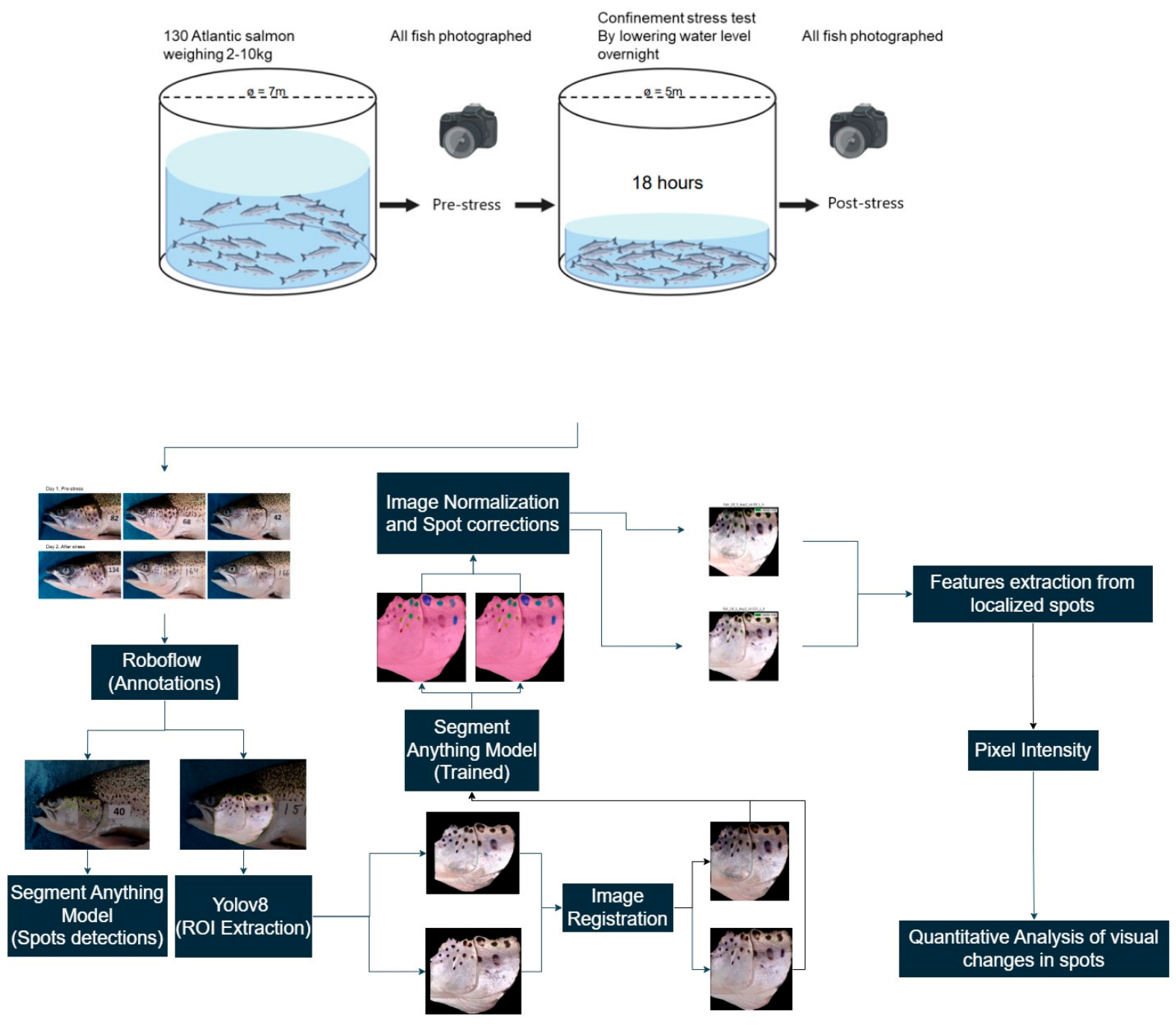
This section describes the experimental setup for data collection, the annotation process used to identify operculum regions and spots, and the use of image augmentation techniques to expand the annotated dataset. It also explains the fine-tuning of models using these annotations for operculum and spot segmentation, followed by the inference process with the fine-tuned models to assess visual changes in the spots. The methodology pipeline can be seen in Figure 1.

3.1. Experimental Setup and Dataset

A total of 130 Atlantic salmon from a commercial breeding program (Aquagen AS, Trondheim, Norway), with a mean age of approximately 2.2 years and body mass ranging between 2 and 10 kg, were used in this experiment. The fish were kept in a circular tank (7 m diameter) with dark green coloration and a continuous supply of UV-light-illuminated seawater pumped from a depth of 90 m, maintained at a constant temperature of 8.9 °C at the Matre Research Station, Institute of Marine Research (IMR), Matredal, Norway.
On the first day, unstressed control fish (n = 8) were captured individually by netting and administered a lethal dose of anesthetic (unbuffered MS-222; 1 g/L). We were only able to use eight unstressed control fish in our experiment, because netting itself can cause stress. They were photographed on both sides of the body, and close-up images of the head were also captured using an Olympus Corporation TG-6 camera model with settings set to auto. The camera was mounted on top of an improvised photo booth made from a wooden frame, with white tarpaulin covering the top, back, and both sides and a fluorescent light source providing illumination from above. The front of the booth was open, so ambient natural sunlight could affect the interior illumination. The remaining fish (n = 122) were sedated and photographed in the same manner as the control fish. Following photography, these fish were transferred to a new tank and subjected to confinement stress overnight (approximately 18 h) by lowering the water level. During confinement, the water depth was approximately 10–15 cm at the edge of the tank. In most fish, the dorsal fins were above the water surface, and the largest individuals were unable to remain upright when attempting to swim near the tank wall.
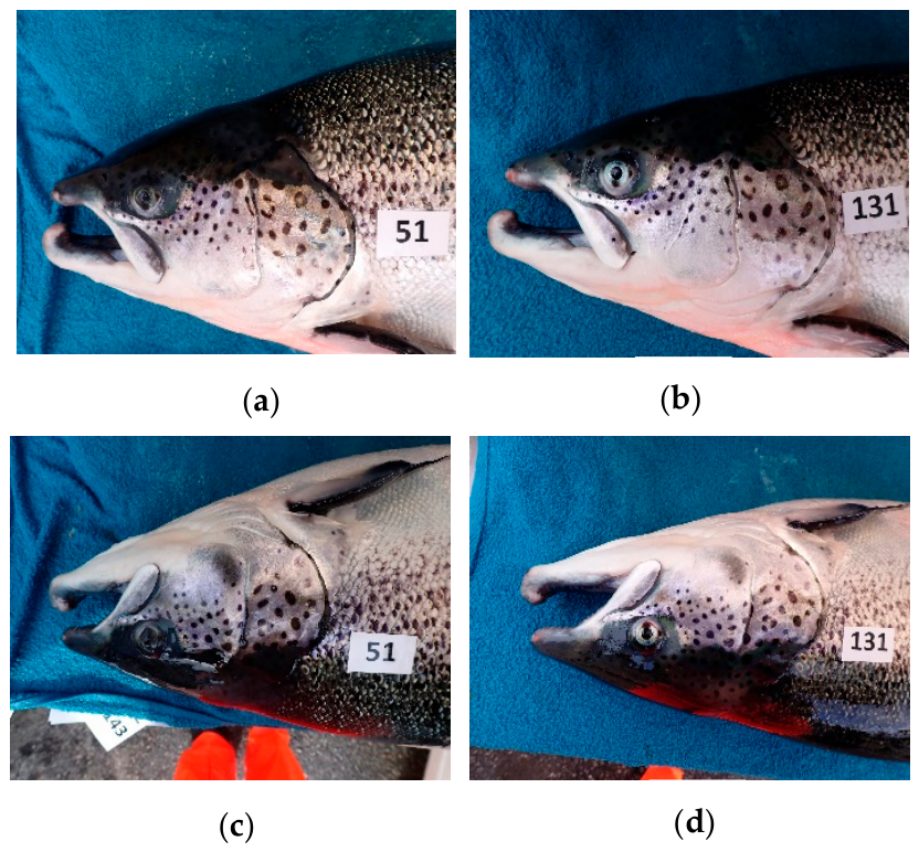
After overnight confinement stress, fish were captured individually using a net, and groups of five to six fish at a time were placed in a 1 m3 container with seawater, after which they were administered a lethal dose of anesthetic and photographed. A total of 1040 images were captured, comprising eight images per salmon, and were further categorized into head and body images. In this study, only the 520 head images were utilized, as these clearly captured the operculum region at close range and allowed spots to be distinctly visible. Only operculum spots were selected due to their prominence and suitability for semi-automated methodology. The pre- and post-stress head images of the same salmon specimen can be seen in Figure 2.

3.2. Image Annotations and Augmentations

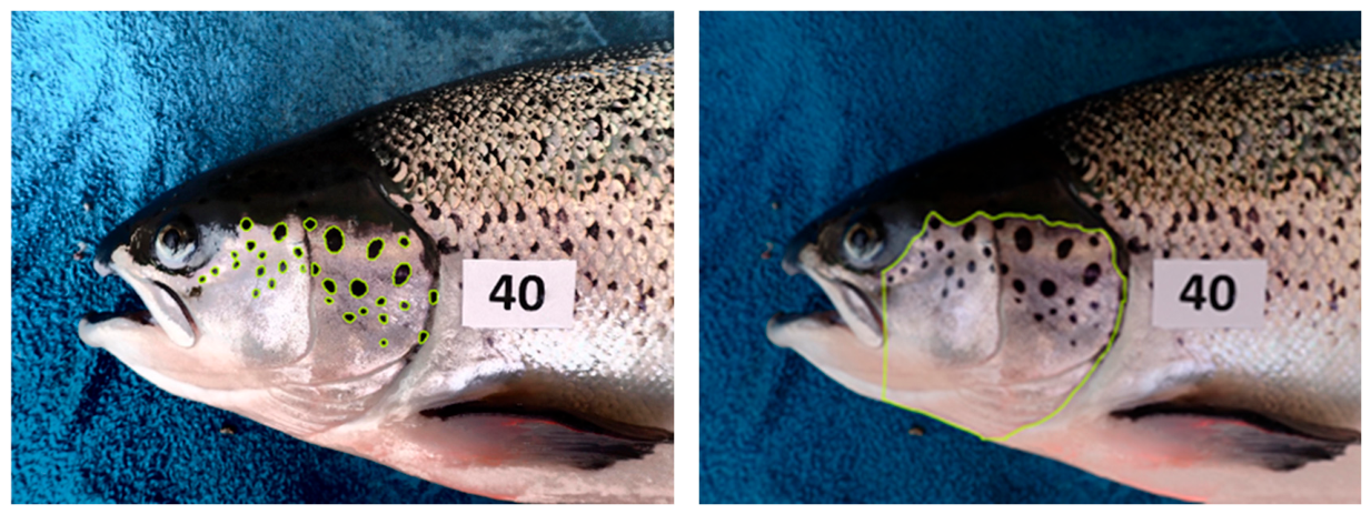
The training of the pretrained models for detection and segmentation of operculum regions and spots was supported by annotating the operculum (Figure 3; right) and spots regions (Figure 3; left) in 275 close-up head images using Roboflow’s annotation toolkit [68]. Spots were annotated based on an instance segmentation strategy aiming to handle variations in shape, size, and texture. Moreover, to facilitate both the detection and semantic segmentation of spots [69], the operculum region was annotated using standard polygon tool; similarly, spots on the operculum were annotated with both standard and smart polygon tools (based on Segment Anything Model (SAM) [70]). A total of 9000 spots (32 spots per fish) and 275 operculum regions were annotated. The annotated operculum regions were split into 70% training (193 images), 20% validation (55 images), and 10% testing (27 images) sets. Geometric and pixel intensity transformation [71]-based augmentations available in Roboflow were applied to the annotated spots images. The motivation behind applying augmentation was to build a dataset with increased variation in shape, size, and texture of spots. The explanation against the augmentation strategies used are as follows.

3.2.1. Geometric Transformations

  • Reflection: Clockwise, counterclockwise, and upside-down reflections were generated with their respective transformation matrices using the following equation:
I m a g e x , y = c e n t e r + i = 0 w i d t h j = 0 h e i g h t I m a g e i , j c e n t e r × M 1 2 3
where c e n t e r = [ w i d t h 2 , H e i g h t 2 ] and M 1 =   0 1 1 0 ,   M 2 = 0 1 1 0 ,   M 3 = 1 0 0 1 are the clockwise, counterclockwise, and upside-down reflection transformation matrices, respectively, and the image spatial resolution is width = 1080, height = 1080.
  • Rotation: Images were randomly rotated using angles (ϴ) randomly sampled from a given range = [−15°, 15°] using the following transformation equation:
I m a g e x , y = c e n t e r + i = 0 w i d t h j = 0 h e i g h t I m a g e i , j c e n t e r × M r o t
where M r o t = c o s ( ϴ ) s i n ( ϴ ) s i n ( ϴ ) c o s ( ϴ ) is the rotation transformation matrix.
  • Shear: Shearing was applied in both horizontal and vertical directions using angles (ϴ) randomly sampled from a given range= [−10°, 10°].
  • Crops: Crops were generated with a randomly sampled zoom factor percentage (zf_perc) within a given range= [0, 10%] using the following transformation:
i d x = I N T w × h × z f _ p e r c w
C r o p = I [ i d x : w + i d x ,   i d x : h + i d x ]
where idx is the zoom factor index along which pixels in horizontal (w) and vertical (h) directions of the image ( I ) are sampled for the crop.

3.2.2. Pixel Intensity Transformations

  • Exposure: Image exposure in both directions was randomly adjusted by randomly sampling a threshold from a given range = [−2%, 2%] using the following transformation equations:
I L A B c v t C o l o r L A B ( I R G B )
I L ; I A ; I B s p l i t ( I L A B )
e x p o s u r e = t h r e s h o l d 255
I L _ a d j u s t e d ± e x p o s u r e
I L A B m e r g e ( I L _ a d j u s t e d ; I A ; I B )
I R G B c v t C o l o r ( I L A B )
where cvtColor, spit, and merge are the color space conversion, channel-wise splitting, and channel-wise merging OpenCV [72] functions. I R G B is the image in RGB color space [73], and I L A B is the variant of the same image in LAB color space [73].
  • Brightness: Brightness adjustment was the same as exposure adjustment, except instead of utilizing the LAB color space, the RGB images were converted to HSV color space [73], and the value channels of the converted images were adjusted.
  • Blur and Noise: Blur was introduced using a Gaussian filter [74], while for noise, salt-and-pepper noise [75] was used.
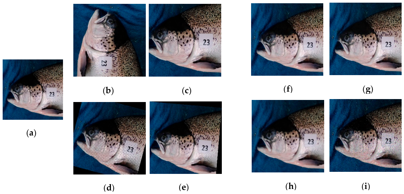
The augmentations (Figure 4) were applied randomly to training images. Geometric transformations such as reflection, rotation, and shearing render the model invariant to camera orientation-related variations, while cropping improves model resilience to variations in the size and positioning of the spots and operculum regions. Pixel intensity transformations such as exposure, brightness, and blur were used to improve model robustness to varying lighting conditions and resilience to camera focus. Lastly, noise was added to help the model against adversarial attacks [76]. The augmented spots training set consisted of 1065 images (approximately representing 35,000 spots), while the validation and test sets were left unaugmented. These augmentations were applied to improve the robustness of the model to variation in spot characteristics (size, pixel intensities, structure, texture, etc.).

3.3. Detection and Segmentation of the Operculum Region and Spots

YOLOv8 [77] and Segment Anything 2 (SAM 2) [78] object detection and segmentation models were used for segmentation of operculum regions and spots within those regions, respectively. YOLOv8 is an object detector comprising three primary components: (i) a backbone, (ii) a neck, (iii) and a head. (i) The backbone includes convolutional blocks, C2f blocks, and a spatial pyramid pooling block. Convolutional block consists of a convolutional layer [36], batch normalization layer [79], and SiLU activation layer [80]. C2f block is further composed of a convolutional block, channel-wise feature map splitting, bottleneck blocks, feature map concatenation, and finally, a convolutional block. The bottleneck block is made up of convolutional blocks with residual connections [62]. Spatial pyramid pooling block [81] consists of a convolutional block, maxpooling layers [36], residual connections, and finally, feature map concatenation followed by a convolutional block. (ii) The neck component is composed of convolutional blocks, c2f blocks, concatenation layers, and transposed convolutional layers [82] for upsampling the spatial resolution of the feature maps. (iii) The head is made up of convolutional blocks and convolutional layers. C2f blocks enable residual learning, which helps mitigate the vanishing gradient problem [62]; it is also responsible for learning a hierarchical representation of the data that captures both textural and semantic information. The spatial pyramid pooling block is responsible for learning multi-scale features, which renders the model invariant to differently sized and scaled objects. The neck is responsible for further refining the multi-scale features for better detections. Finally, the head component is responsible for predicting bounding box coordinates [83], segmentation masks [83], and class labels [83] against the detections. State-of-the-art segmentation model, Segment Anything 2 (SAM 2), is composed of the following architectural components: (i) image encoder, (ii) memory attention, (iii) mask decoder, (iv) prompt encoder, (v) memory encoder, and (vi) memory bank. (i) Image encoder is based on Hiera image encoder [84], which is mainly composed of 4 hierarchical vision transformers (ViT) [85] termed as 4 stages of the architecture. Two of those stages’ feature maps are fused using a feature pyramid network [86] to produce embeddings against an input image. (ii) Memory attention block is made up of a stack of transformers [87] responsible for self-attention [88] and follow-up cross-attention [89] with memory embeddings. (iii) Prompt encoder follows [70] encoder-enabling prompts through clicks, bounding boxes, and masks. (iv) Mask decoder architecture also largely follows [70] a decoder with its bi-directional transformer blocks approach to prompt self-attention and cross-attention between prompt-to-image embedding and vice versa. (v) Memory encoder reuses the image embedding generated by the image encoder and fuses it with the downsampled version of the previously generated mask to generate a memory. (vi) Memory bank is based on the first-in-first-out (FIFO) queue of previously generated memories (including images (frames) and prompts) against previously predicted objects. Image encoder generates image embeddings for a given image, which is conditioned on previous frames and their respective predictions by the memory attention block. Mask decoder takes prompt information along with information provided by the memory attention block for generating a prediction for a given image.

YOLOv8 and SAM2.1 Training

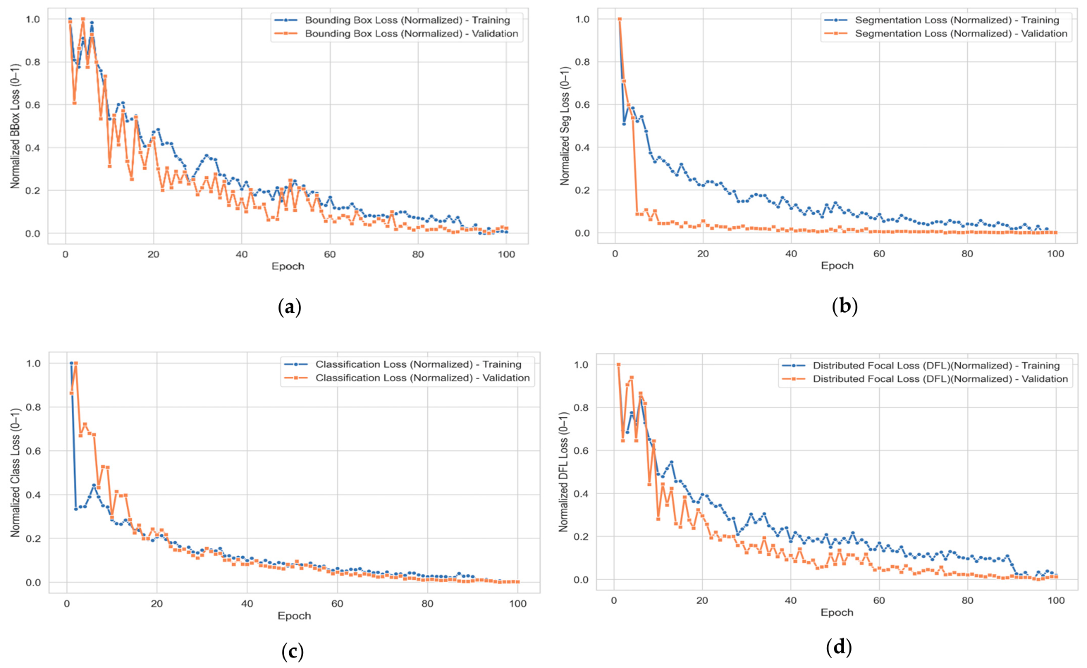
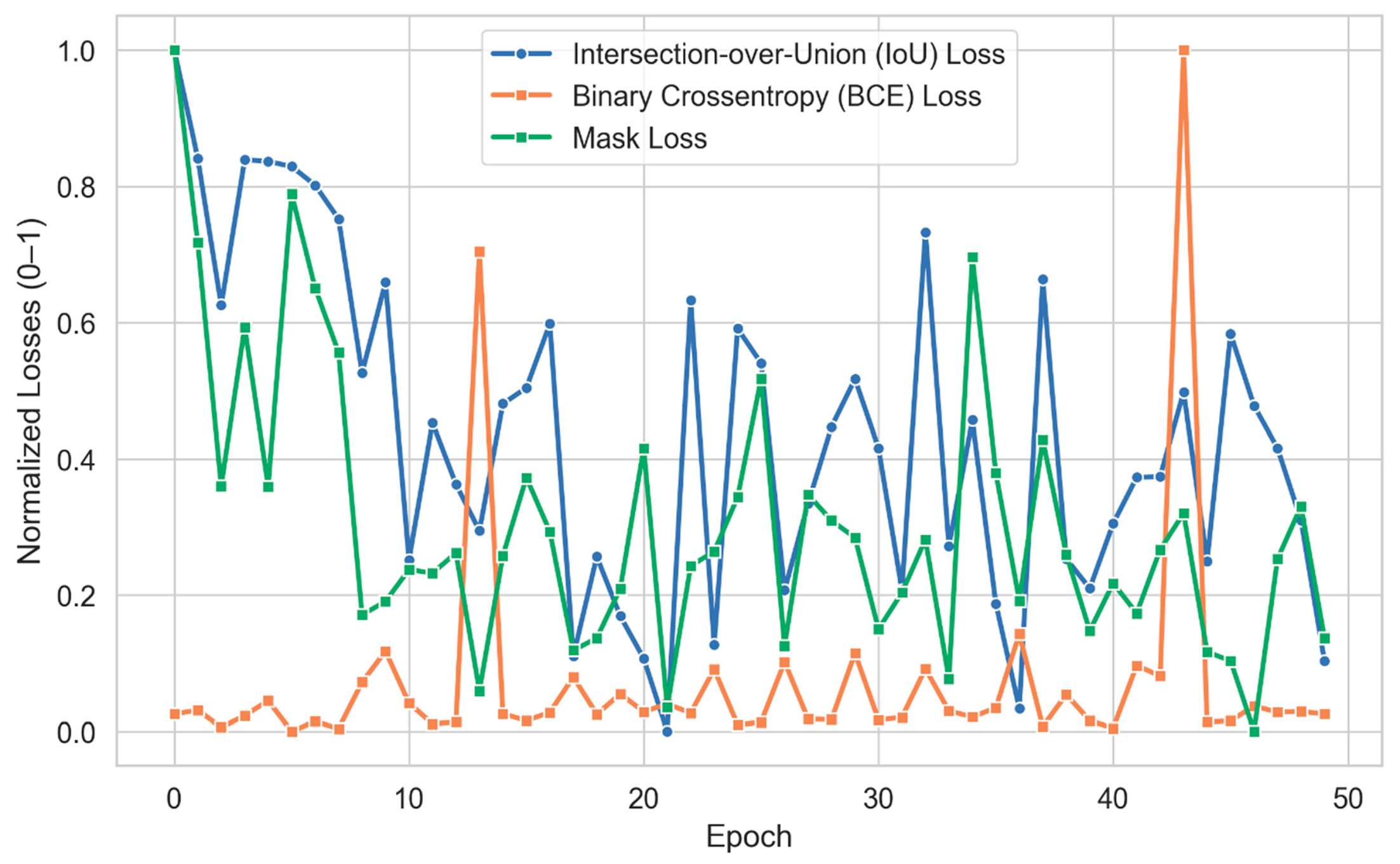
Pretrained Yolov8 [63] for operculum region segmentation was retrained on non-augmented operculum images dataset with Ultralytics [45] library. During retraining, a spatial resolution of 1080 × 1080 was adopted with a batch size of 4. The whole training duration lasted 100 epochs, with training epochs set to 100, with 25 early stopping rounds for mitigating overfitting [90], along with a dropout rate of 20%. Adam optimizer [91] with a learning rate of 0.002 and momentum of 0.99 was used for fine-tuning the model. The default data augmentations via the albumentations library [92] such as Gaussian blur, CLAHE, grayscale conversion, and an 8 × 8 tile-size adjustment were used during fine-tuning. The comprehensive list of other data augmentations applied during training of the model can be seen in Table 1. The model was evaluated on a set aside validation set with metrics such as recall [93], precision [93], and mean average precision (mAP) [93]. The training and validation losses of the model can be seen in Figure 5 with segmentation loss exhibiting underfitting, which could be the consequence of using a 20% dropout rate. SAM2.1 (pretrained Hiera-B+ [84]) was fine-tuned with an augmented dataset of spots for 40 epochs. Precision (Equation (5)), recall (Equation (6)), and mean average precision (Equation (7)) metrics of YOLOv8 are mentioned in Table 2. Binary cross-entropy (Equation (8)) and intersection-over-union (Equation (9)) and mask losses average over 40 epochs of SAM are mentioned in Table 3. It can be seen in Figure 6 that the different losses of SAM2.1 model converged near the completion of the epochs.
R e c a l l = T P T P + F P  
P r e c i s i o n = T P T P + F N  
m e a n a v e r a g e   P r e c i s i o n = 1 C   i = 1 C t = 1 T ( R e c a l l t R e c a l l t 1 ) P r e c i s i o n t  
where TP, FP, and FN are true positives, false positives, and false negatives. C is the total number of classes (in our case, 1 roi—region of interest (operculum)), and T is the threshold on which the recall and precision are computed (typically set to 0.25).
B i n a r y   C r o s s e n t r o p y   B C E   L o s s = 1 N i = 1 N [ y i log p i + 1 y i log ( 1 p i ) ]  
I n t e r s e c t i o n o v e r U n i o n   I o U   L o s s = 1 N i = 1 N ( 1 B b o x g t 1   B b o x p r e d i B b o x g t 1   B b o x p r e d i )  
where y , p are the ground truth mask class labels and predicted probabilities against observations belonging to a class. N is total number of observations. B b o x p r e d ,   B b o x g t   are predicted and ground truth bounding boxes.

3.4. Inference

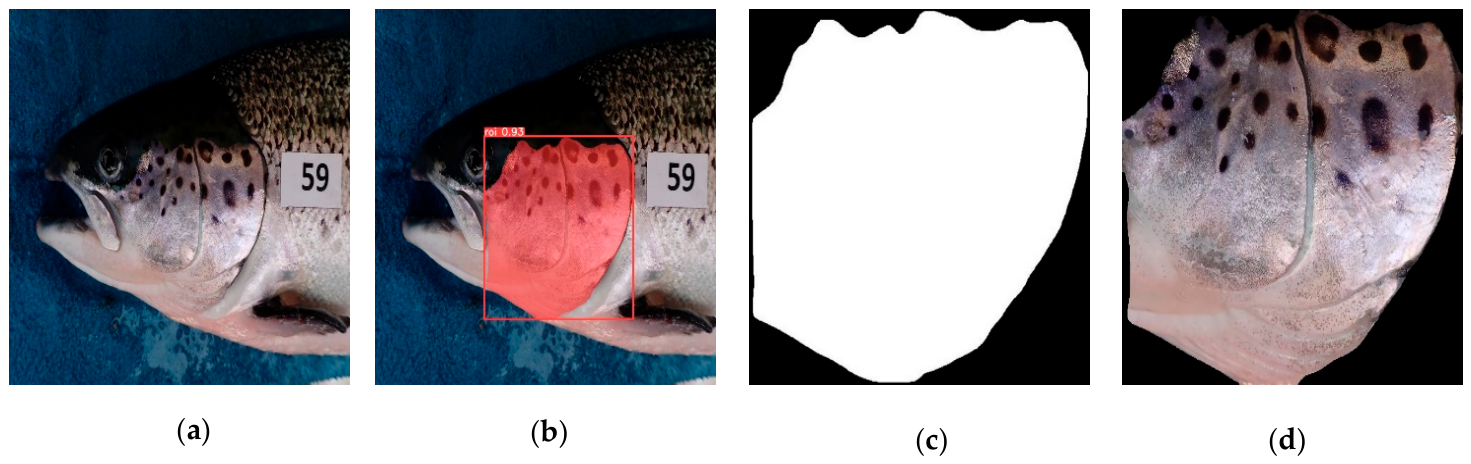
At inference, an unseen dataset consisting of 84 images collected from 21 stressed (treated) salmon specimens with each one photographed 4 times (left side: pre-, post-stress; right side: pre-, post-stress) was used. Operculum regions from these images were extracted through binary masks obtained from the trained YOLOv8 (Figure 7).

3.4.1. Operculum Regions Registration

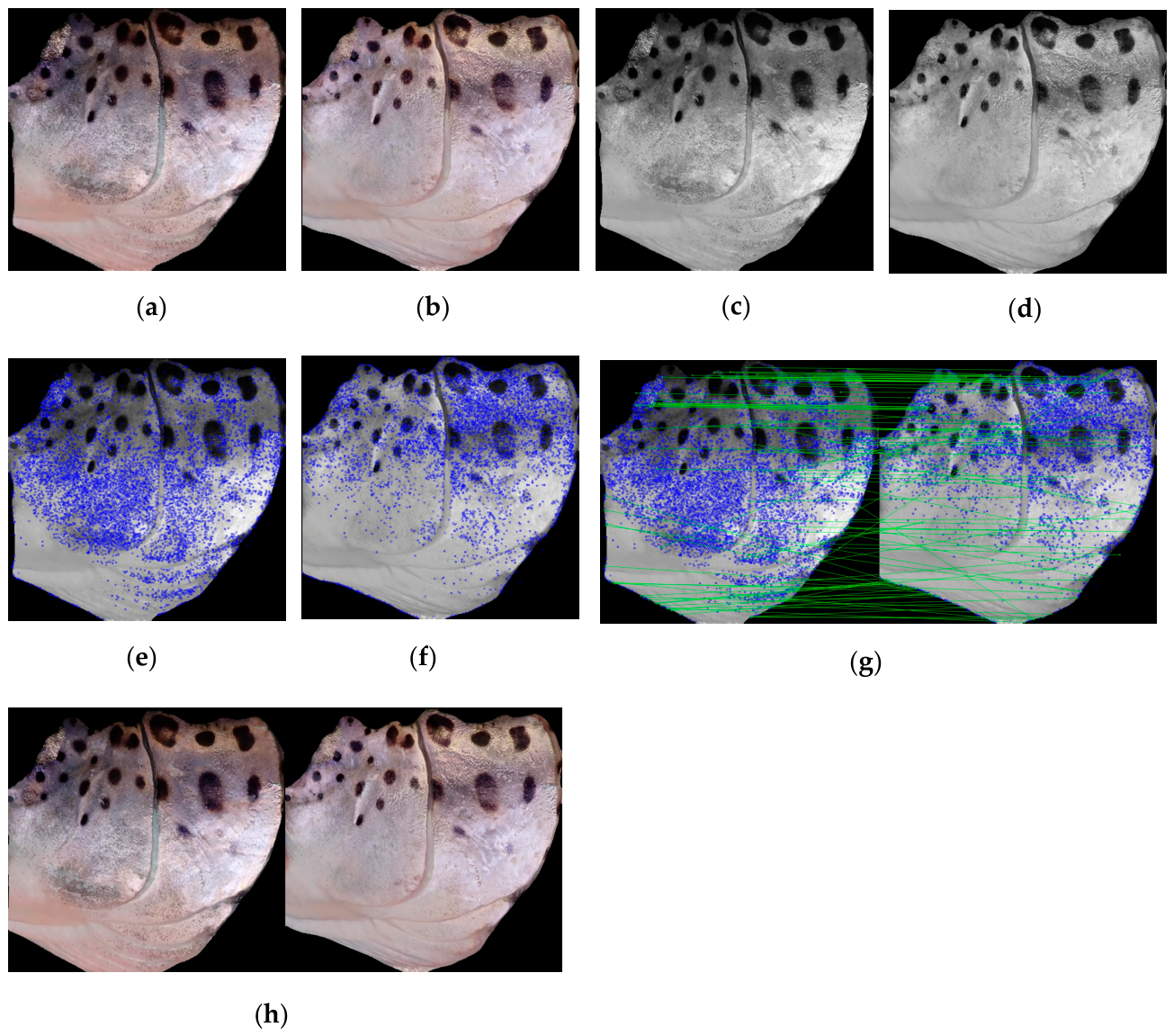
The extracted operculum regions were sorted into pre- and post-stress groups and registered to ensure some degree of 1 to−1 correspondence between them for pre- and post-stress visual changes in spots analysis later. The image registration pipeline is based on the OpenCV library [72]: (i) Pre- and post-stress regions sidewise (left and right) are converted to grayscale, (ii) scale-invariant feature transform (SIFT) [58] feature detector is used to detect and compute the feature keypoints and descriptors, respectively, in the pre- and post-stress grayscale regions, (iii) fast library for approximate nearest neighbors (FLANN) [94]-based matcher is used to match the feature descriptors, (iv) Lowe’s ratio test [58] is applied to sample the best matches for corresponding keypoint extraction, (v) the extracted keypoints with RANSAC [95] are used to compute the homography matrix [96], and (vi) the matrix is applied to the pre-stress region and aligned with the post-stress region. The different stages of the registration pipeline can be seen in Figure 8.

3.4.2. Operculum Regions Normalization

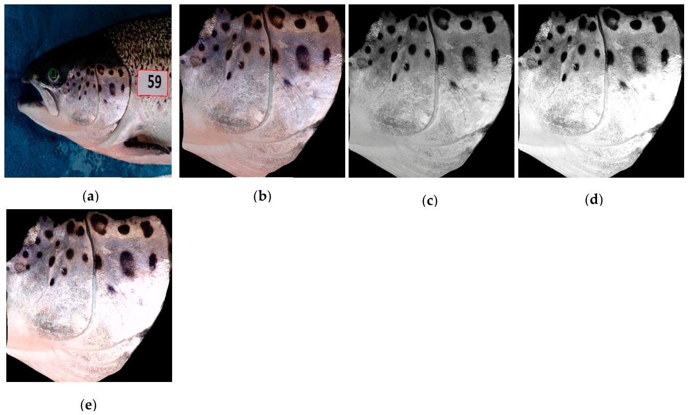
The unseen dataset was photographed in conditions similar to model training and evaluation datasets. The registered regions were normalized with grayscale adaptation of the white patch retinex algorithm [97,98]: (i) The eye and ID-tag regions of the salmon specimens were manually annotated with the smart polygon tool available in Roboflow [68]. (ii) Black pixels in segmented eye regions were sorted in ascending order, and 20% of pixels were sampled, averaged, and used as reference black pixels ( β ). (iii) White pixels in segmented ID-tag regions were sorted in descending order, and 20% of pixels were sampled, averaged, and used as reference white pixels ( α ). (iv) Each RGB salmon specimen operculum region image was converted to LAB color space, the luminance (L) channel was extracted, and bias correction was applied using averaged black reference pixels, while contrast was adjusted with averaged white reference pixels. (v) Furthermore, the pixels in L-channel were clipped between 0 and 255. (vi) Finally, the normalized L-channel of the image was merged back with the left-out channels (i.e., A and B) and converted back to RGB color space. The normalization algorithm output can be seen in Figure 9. The mathematical equation for image normalization can be seen in Equation (10).
I n o r m x , y = min max 0 , I i , j β α , 255        

3.4.3. Operculum Region Spots Segmentation

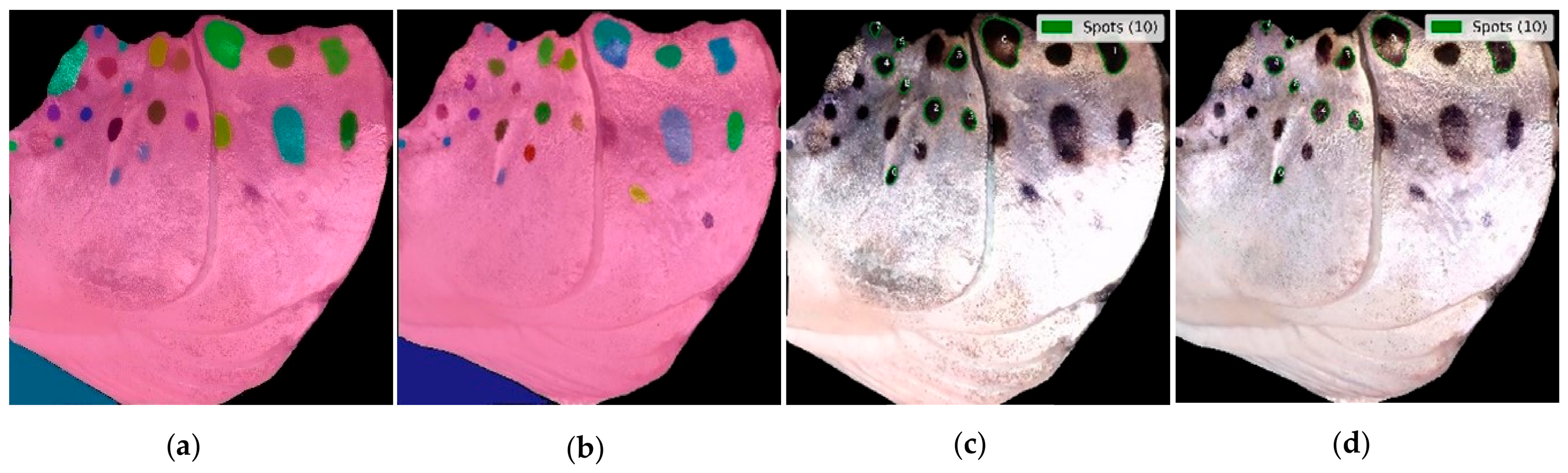
Registered and normalized operculum region images were used to obtain spot localization information (bounding boxes, masks) from the fine-tuned SAM. Spots (Figure 10) exhibiting specular highlights, complete occlusion due to mucus, and partial occlusion due to water droplets and reflective anomalies were removed from both pre- and post-stress operculum regions in Roboflow. Moreover, misaligned spot contours and missed spots were also manually corrected and annotated, respectively. After the removal of anomalous spots and annotation of missed spots, a total of 676 spots in 84 images corresponding to 21 salmon specimens were identified and rendered fit for grayscale pixel intensity-based spot-wise analysis. These spots were matched in both pre- and post-stress images using the following steps (Figure 11): (i) The center point of each bounding box localizing the spot was computed. (ii) Euclidian distances between pre-stress and post-stress spots were computed (in 1-to-many association). (iii) Minimum distances between pairs of pre- and post-stress spots were computed, and their corresponding labels (segmentation coordinates) were sorted accordingly. (iv) Some of the spots with inaccuracies were handled manually for matching.

3.4.4. Features Extraction

Matched and corrected spot segmentation polygon coordinates were utilized in constructing binary spot masks and were further utilized in feature extraction using the following steps: (i) Operculum images were converted to grayscale images, (ii) segmentation coordinates corresponding to spots in the operculum were used to construct spot binary masks, (iii) grayscale pixels localized by binary masks were sorted into 10 bins of size 0.1, and (iv) individual spot pixel intensities in their respective bins, as well as intensity means computed from all bins, were associated with the respective salmon specimens.

3.4.5. Statistical Analysis (Grayscale Intensity)

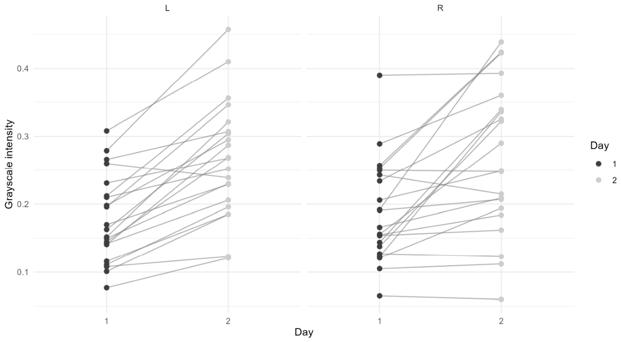
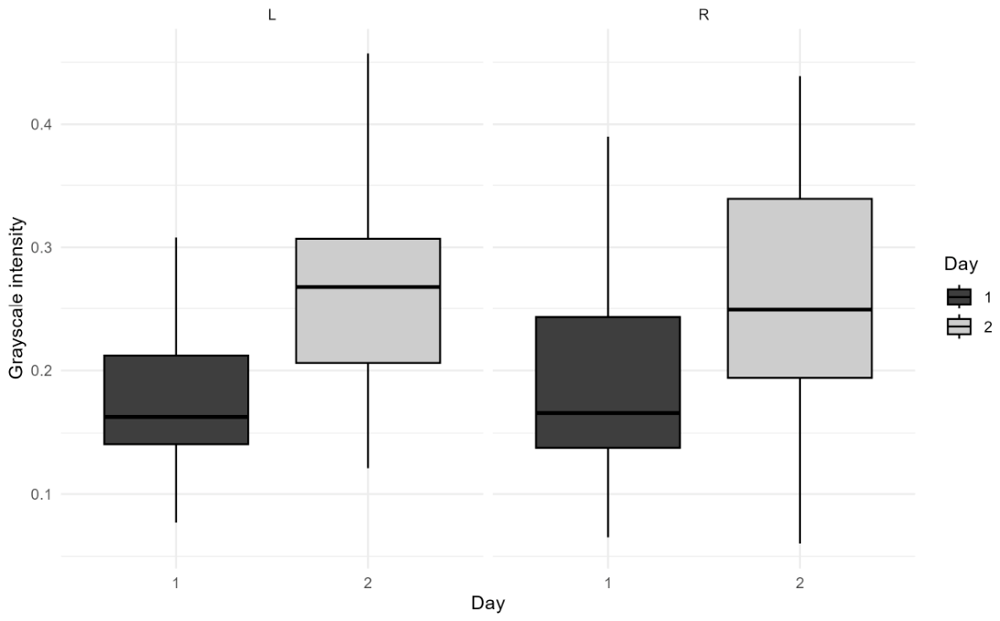
Grayscale pixel intensity was analyzed as a repeated-measure outcome in individual fish, with measurements taken on two different days and on both the left and right sides. Since the grayscale intensity is a continuous variable bounded between 0 and 1, and because repeated observations within fish are not independent, the data were modeled using a beta-mixed-effects model fit by maximum likelihood. The model included the day, side, and their interaction as fixed effects, with fish identity as a random intercept to account for within-fish correlation. The mean grayscale intensity increased from Day 1 to Day 2 on both left (0.178 to 0.266) and right sides (0.189 to 0.267). Consistent with this pattern, there was a significant effect of day ( β = 0.514, SE = 0.101,   z = 5.15, p-value = 2.66 × 10⁻⁷ ( p < 0.001), and 95% CI 0.320–0.714), indicating higher grayscale intensity at Day 2, whereas neither side ( β = 0.0585, p = 0.582) nor the day × side interaction ( β = −0.0653, p = 0.644) was statistically significant. Model-based estimated marginal means similarly showed higher grayscale intensity at Day 2 for both sides. Across paired observations, the mean absolute increase in grayscale intensity was 0.083 (95% CI 0.061–0.105), corresponding to a mean relative increase of 50.5% (95% CI 36.5–64.4). Together, these results indicate a clear temporal increase in grayscale intensity, with no evidence that the magnitude of change differed between the left and right sides. The likelihood-based mixed-model framework is appropriate for bounded repeated-measure data; the modest sample size and variability in individual-level change should be considered when interpreting the strength and generalizability of these findings. The individual trajectories and the boxplot of the grayscale intensities grouped by side and day can be seen in Figure 12 and Figure 13, respectively.

3.4.6. Cortisol Assay

Plasma cortisol concentrations were quantified using a commercially available enzyme-linked immunosorbent assay (DetectX® Cortisol ELISA Kit, Arbor Assays™, Ann Arbor, MI, USA) following the manufacturer’s protocol. Plasma samples (5 µL) were diluted 1:100 prior to analysis, and absorbance was measured at 450 nm using a microplate spectrophotometer (Epoch, Agilent Technologies, Santa Clara, CA, USA) with Gen5 v3.00 software. Concentrations were interpolated from duplicate eight-point standard curves (50–3200 pg mL−1) fitted using a four-parameter logistic model (R2 = 0.998). Assay precision was high (intra-assay coefficient of variation: 4.62 ± 0.57%, mean ± SEM), and antibody cross-reactivity was reported as 100% for cortisol and <20% for other steroids.
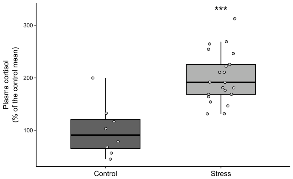
To facilitate comparisons among experimental treatments, cortisol values were standardized relative to the control group. Specifically, the mean cortisol concentration of control individuals was calculated, and all individual values (control and stress treatment) were expressed as a percentage of this mean. Subsequent analyses therefore focused on relative differences between treatments rather than absolute hormone concentrations.
Statistical Analysis (Plasma Cortisol)
Cortisol levels (percentage of control mean) were compared between control and stress treatments using a non-parametric Wilcoxon rank-sum test. Data are presented as medians and interquartile ranges (IQRs), and tests were two-tailed with α = 0.05.
Cortisol levels, expressed as a percentage of the control mean, were significantly higher in the stress treatment compared to the control group (Wilcoxon rank-sum test: W = 14, p < 0.001). Median cortisol values were approximately twofold higher in stressed individuals (median = 192%, IQR = 57.6) than in controls (median = 90.9%, IQR = 55.3), confirming that the stress treatment elicited a physiological stress response (Figure 14).

4. Results

4.1. Effect of Treatment on the Spot Pixel Intensities

The grayscale pixel intensities of the spots on Day 1 and Day 2 were averaged separately, and the change in mean pre-stress and post-stress spot pixel intensity in the operculum region was calculated using the following equation:
C h a n g e =   M e a n   P i x e l   I n t e n s i t y   D a y   2 M e a n   P i x e l   I n t e n s i t y   ( D a y   1 )   M e a n   P i x e l   I n t e n s i t y   ( D a y   1 )
As shown in Table 4, the response to treatment was heterogeneous across individuals. Several fish showed moderate increases in spot pixel intensity, whereas others showed very large increases, and a few showed negative changes, indicating reduced post-stress intensity relative to pre-stress values. The mean percentage change was positive on both sides, suggesting an overall treatment-associated increase in spot pixel intensity; the widespread values point to considerable inter-individual variation.

4.2. Grayscale Intensities of Treated and Control Groups

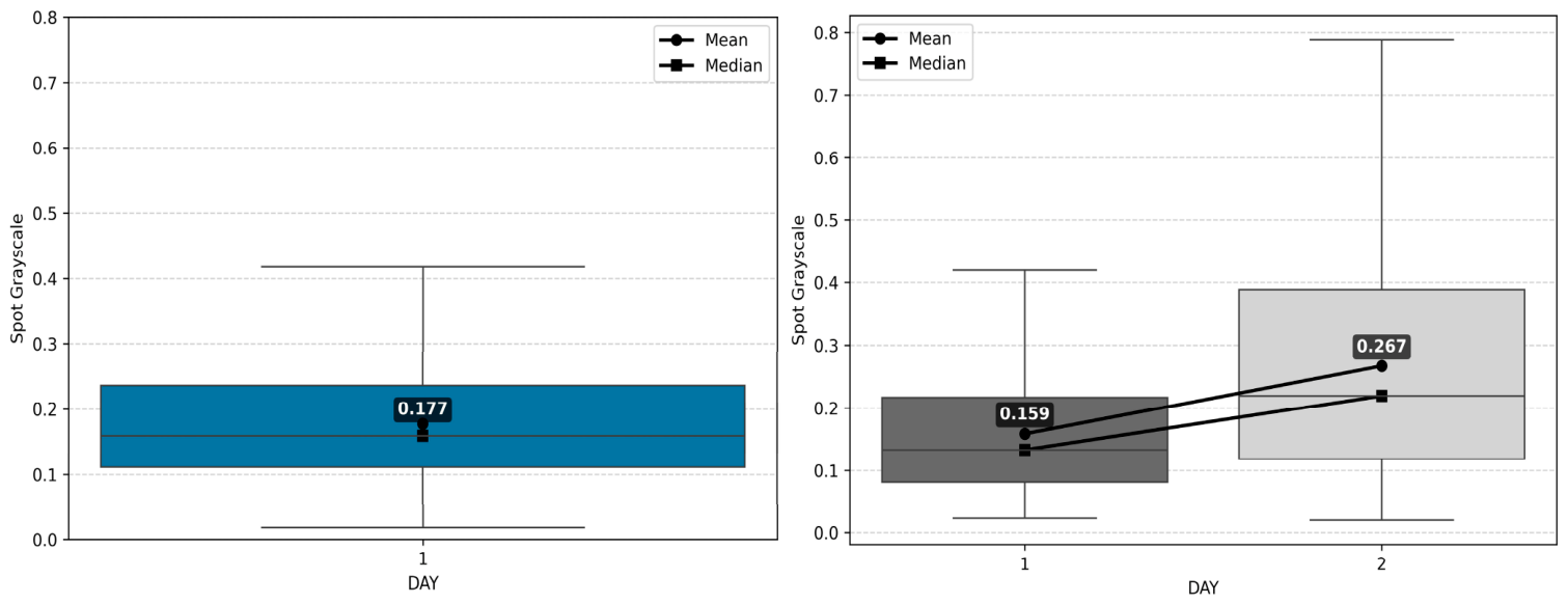
The spots sampled from eight control fish and 21 treated fish were analyzed for outlier removals. The lower bound and upper bound of the extracted features were computed using the following steps: (i) The interquartile range (IQR) was computed utilizing the Q1 (25th percentile) and Q3 (75th percentile) of the data, (ii) the lower (Q1—factor * IQR) and upper (Q3—factor * IQR) bounds were computed with a factor of 1.5, (iii) feature values falling below the lower bound or above the upper bound were identified and removed, and (iv) this process was repeated for 10 iterations to remove all of the outliers from the grayscale intensities. After the removal of outliers, the remaining grayscale intensities were plotted. In Figure 15, we can observe that the distribution of control and pre-stress spots exhibited a similar spread, with an interquartile range (IQR) of approximately 0.12. In contrast, increased variation is observed in the post-stress spots, indicating greater dispersion in grayscale intensity values. We can also observe that the mean value on Day 2 is higher than Day 1, indicating that, on average, the spots are becoming brighter on Day 2.

4.3. Neighborhood-Based Grayscale Intensity Analysis

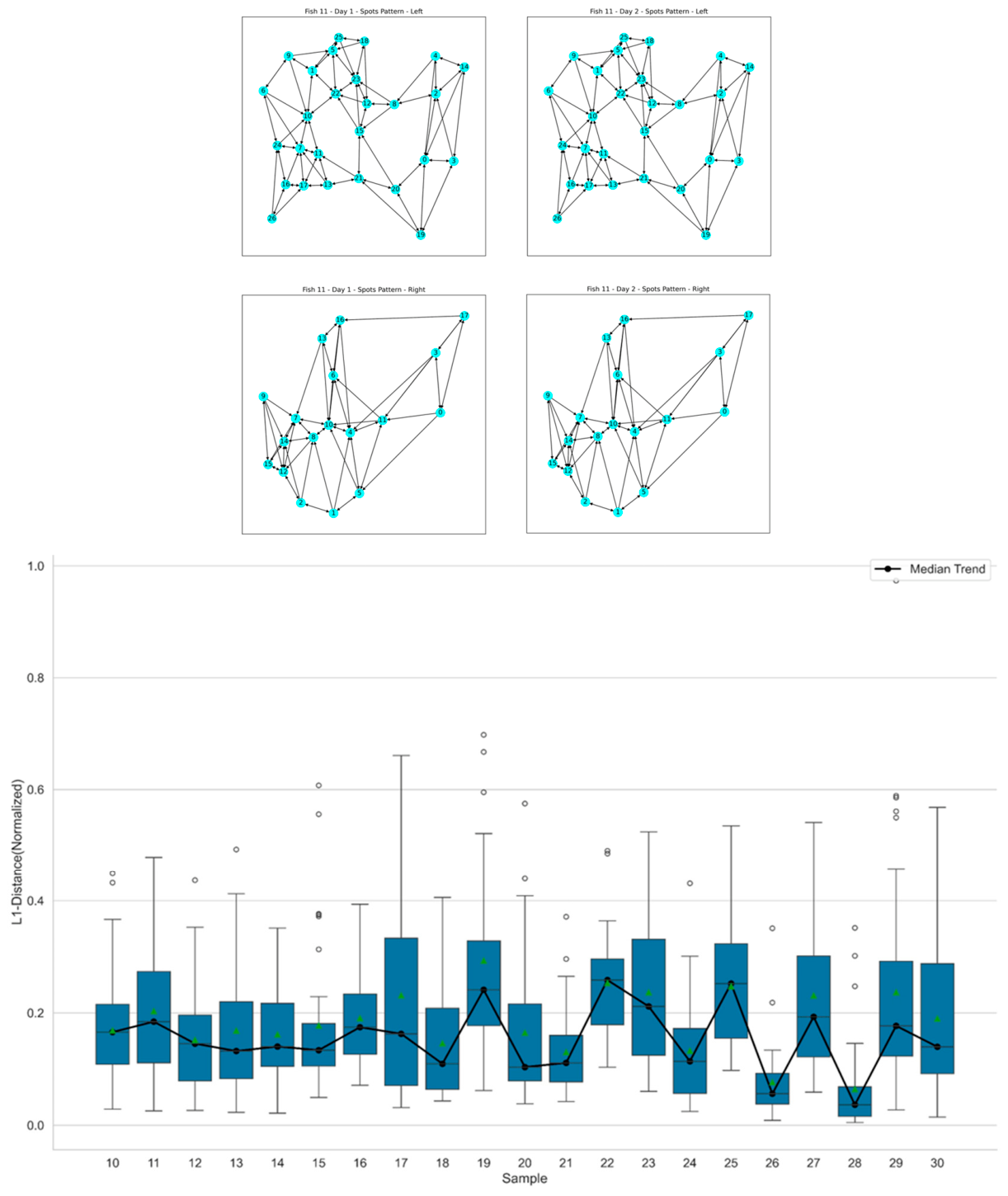
Grayscale pixel intensities of 676 spots and their neighbors were analyzed on Day 1 (pre-stress) and Day 2 (post-stress) using the following steps: (i) The center points of bounding boxes localizing spots were used to compute the Euclidean distances between a spot (source) and the remaining spots (targets) in each operculum region with respect to side and day (1: pre-stress; 2: post-stress). (ii) Distances between the source and target spots were sorted in ascending order, and four neighbors per spot were extracted. (iii) Coordinates of the source and neighboring spots were used to construct directed graph visualizations [99] (Figure 16; top) for each operculum–day–side combination. (iv) The differences in pixel intensities between the source and target spots for each operculum–day combination were formulated in source-wise 1-D vectors. (v) Normalized L1 distances [57] (0: similar; 1: completely different) between source vectors on Day 1 and Day 2 were computed. These normalized L1 distances were used to construct boxplots (Figure 16; bottom) for each salmon specimen. The variation observed within each specimen reflects the inter-individual differences in changes in spot intensities relative to their neighboring spots on Day 2.

4.4. Manual Scoring of Spots on a Grayscale by Observers

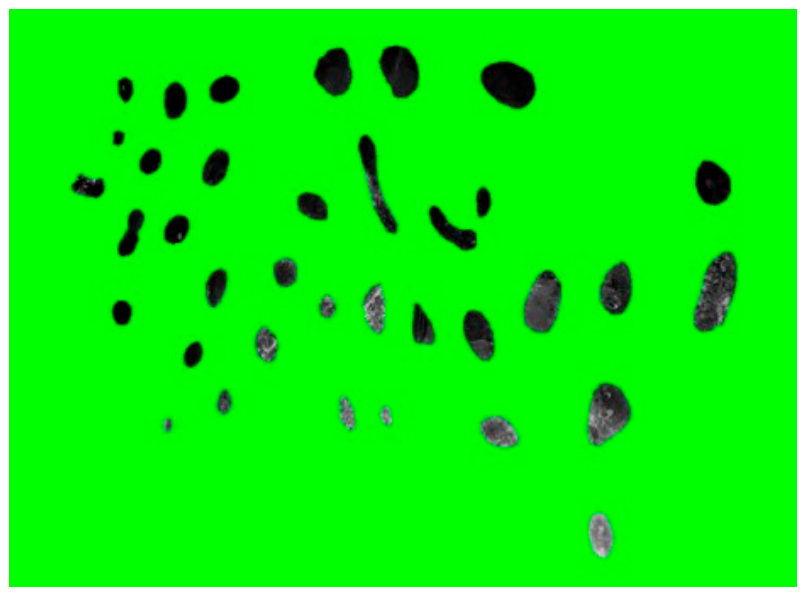
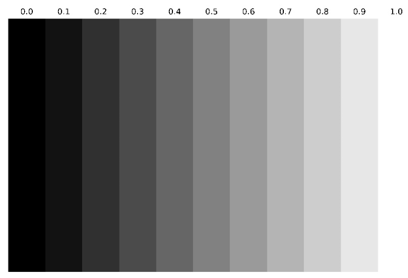
A composite–image generation pipeline was developed to visualize annotated spot regions across matched pre- and post-stress image sets. For each fish sample, four (left Day 1 and 2, right Day 1 and 2) grayscale images were loaded together with their polygon-based spot annotations. A parameter (nspots) was defined to include all annotated spots from each grayscale image, such that the full set of available spot regions in each image was incorporated into mask generation. Spot annotation coordinates, originally represented in normalized form, were transformed into pixel-space coordinates using the dimensions (height, width) of the corresponding source image. These polygons were subsequently rasterized to produce binary masks for each of the four images. To ensure adequate spot region representation, the resulting masks were evaluated against a minimum pixel-area criterion before inclusion in the final visualizations. The four grayscale images and their corresponding binary masks were then assembled into 2 × 2 stitched images. From these composites, a stitched green background, spot-placeholder image was rendered, with all annotated spots from the four images for each fish sample represented individually. The pre-stress spots on a green background can be seen in Figure 17.
The stitched images were printed on A4 sheets, and two observers manually scored the spots on a grayscale (Figure 18). It can be observed in Table 4 and Table 5 that algorithm-driven and manual grayscale change scores showed similar central tendencies on the left side, with mean values of 54.83 and 52.69 for the two observers and 54.5 for the algorithm. Agreement between the algorithm and manual scoring was moderate for left-sided spots, indicating that the automated method broadly captured the direction and magnitude of observer-assessed changes in the pre- and post-stress spots. In contrast, right-sided scores were substantially more variable, with wider ranges of values in the manual assessments. Although the algorithmic mean right-side value was 46.5 and the two manual means were 52.52 and 65.15, the concordance with manual scoring was weak. This discrepancy on the right side is interestingly unknown to us. However, the algorithm appeared to compress the range of scores, tending to overestimate low values and underestimate extreme values relative to human observers.
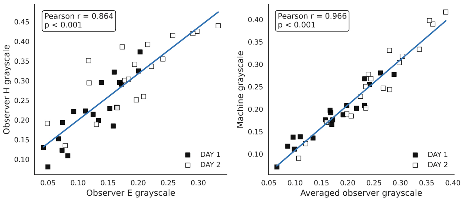
Furthermore, to reduce inter-observer variability, grayscale absolute values from the left and right sides were averaged for each observer and compared both between observers and against the machine-derived grayscale values averaged across sides using Pearson correlation analysis.
Pearson correlation analysis showed a strong positive association between Observer E’s and Observer H’s measurements (r = 0.864, p < 0.001), indicating strong inter-observer agreement. A stronger positive association was observed between the averaged observer measurements and machine-derived values (r = 0.966, p < 0.001), suggesting that the machine measurements closely matched the consensus manual assessment. These relationships were consistent across Day 1 and Day 2. The scatter plots for both analyses can be seen in Figure 19.

5. Discussion and Future Research

The main objective of this study was to investigate whether changes in the grayscale intensity of melanin-based skin spots on the operculum of Atlantic salmon could be detected using a semi-automated computer vision pipeline. The results indicate that such changes can be quantified from out-of-water images collected before and after the applied confinement episode. Across the analyzed fish, the mean grayscale intensity of opercular spots increased from Day 1 to Day 2, and the mixed-effects analysis supported a significant temporal effect. At the same time, responses varied substantially among individuals, indicating considerable heterogeneity in the magnitude and direction of change.
The findings suggest that the proposed methodology is sensitive to changes in spot appearance under the present experimental conditions. The confinement challenge was intended to elicit a stress response, and the independent physiological stress marker (plasma cortisol) was evaluated. It was observed that cortisol levels appeared elevated in the treated fish relative to controls, confirming that the experimental manipulation elicited a physiological stress response. The magnitude of this difference was lower than that reported in studies of acute confinement stress in Atlantic salmon, where marked increases in plasma cortisol are observed following short-term exposure (e.g., 30 min; [100]). This potentially reflects differences in sampling context. Cortisol responses are transient and can be rapidly induced by minor disturbances (e.g., netting and handling; [101]), such that control individuals may not represent true baseline levels but rather fish that were not exposed to the experimental stress challenge. In addition, the prolonged stress exposure applied here may have reduced the magnitude of the observed difference relative to acute stress paradigms.
In addition, the applied challenge may have involved confounding factors that could also have influenced pigmentation, including altered brightness conditions, body positioning, and context-dependent color responses. Fish coloration is known to vary for multiple reasons, including background adaptation, social signaling, and physiological state [11,20,22,25]. The present design does not fully separate these possible drivers. For this reason, the changes observed in this study should be interpreted as treatment-associated rather than as definitive evidence of a validated stress-specific response. Furthermore, another limitation concerns the control group. Although control fish were included, the sample size was small relative to the treated group, and the comparison between the two groups should therefore be interpreted cautiously. The present study is therefore best understood as a proof-of-principle investigation showing that opercular melanin-based spots appearances can change measurably across repeated imaging points under the applied confinement episode conditions.
Methodologically, the study demonstrates that semi-automated segmentation of the operculum and spot regions is feasible with high accuracy. The trained YOLOv8 model performed strongly for operculum segmentation, and the SAM-based approach enabled detailed spot extraction within the opercular region. These components were essential for constructing a pipeline capable of spot-level quantification. Similar developments in computer vision have already shown considerable promise in aquaculture applications, including wound detection, lice detection, fish monitoring, and pattern-based identification [27,28,29,30,31,60]. The manual correction steps required during inference nevertheless highlight that the workflow is not yet fully automated. Occlusion caused by mucus, water droplets, and reflections still required manual intervention, which limits current scalability and real-time applicability.
Another important consideration is the sensitivity of the entire workflow to imaging conditions. Because the analysis relies on grayscale intensity, any variation in lighting, exposure, focus, viewing angle, or reflective artifacts may influence the extracted features. To reduce this problem, image normalization and visual spots were screened for suitability prior to analysis. We also restricted the study to opercular spots, as these were generally more prominent and more consistently visible than spots in other body regions. Despite these precautions, residual variation related to image acquisition cannot be excluded. The weaker right-side agreement suggests that some aspects of image registration, segmentation consistency, or visual scoring remain insufficiently controlled. At the same time, the positive correlations between the observers and between the observers and the machine-derived grayscale values suggest that the algorithm is generally able to track the direction of change and shows an overall agreement with the manual assessment.
The neighborhood-based analysis provided additional descriptive information by examining changes in spot intensity relative to neighboring spots within the same operculum. The variability observed within and among fish indicates that the response was not spatially uniform. This may reflect local pigmentation dynamics, technical variability in image acquisition and matching, or a combination of both. From a biological perspective, this interpretation remains tentative. Previous work has shown that melanin-based pigmentation in salmonids may be associated with differences in stress responsiveness and other aspects of individual phenotypes [17,18,19], but the mechanisms underlying short-term visual changes in discrete opercular spots are still not completely understood. Although the observed spatial heterogeneity is intriguing, the present study was not designed to resolve the biological basis of localized spot change.
Overall, the results support the view that the image-based quantification of opercular spot appearance may be useful for welfare-related research in Atlantic salmon. The study does not establish opercular spot intensity as a validated biomarker for stress, but it does show that measurable changes in melanin-based spot appearance can be captured using computer vision methods under a defined experimental setup. In that sense, the work provides a methodological foundation for further studies on pigmentation dynamics in salmon.
In the future, we will focus on experimental validation and rigorous control of image acquisition conditions. This includes standardized lighting, camera settings, camera-to-subject distance, and fish positioning. Future experiments will also include larger and more balanced control groups, along with confinement conditions that minimize confounding effects from background adaptation and other coloration responses. In addition, the biological relevance of spot changes should be validated against established physiological stress indicators, such as cortisol and other endocrine or neurochemical markers. Finally, the method should be tested on more diverse datasets spanning multiple stocks, environments, and pigmentation phenotypes to access its generalizability and robustness.
In summary, this study should be viewed as proof-of-principle demonstration that melanin-based opercular spots in Atlantic salmon can be detected, segmented, and quantitatively analyzed using computer vision and that their grayscale appearance may change following exposure to confinement episodes. While the findings are promising, further validation is required before such changes can be interpreted confidently as a stress-specific welfare indicator or translated into practical monitoring applications.

6. Conclusions

This study provides a proof-of-principle demonstration that computer vision can be used to detect, segment, and quantify melanin-based opercular spots and treatment associated changes in their grayscale intensities in Atlantic salmon. The observed changes in grayscale intensity between pre- and post-confinement images show that the method can capture temporal changes in spot appearance under the present experimental conditions. However, the findings should be interpreted cautiously, as stress was not independently validated, and alternative causes of color change were not excluded in this study. Our work establishes a methodological basis for future studies on opercular pigmentation as a potential non-invasive welfare-related indicator.

Author Contributions

Conceptualization, T.L. and Ø.Ø.; Methodology, T.L. and H.U.; Software, T.L.; Validation, T.L., E.A.L.G., H.N.G., Ø.Ø. and H.U.; Formal analysis, T.L.; Investigation, T.L., Ø.Ø. and H.U.; Resources, Ø.Ø.; Data curation, O.F. and J.N.; Writing—original draft, T.L.; Writing—review and editing, T.L.; Visualization, T.L.; Supervision, M.G., Ø.Ø. and H.U.; Project administration, Ø.Ø.; Funding acquisition, Ø.Ø. All authors have read and agreed to the published version of the manuscript.

Funding

The study is funded by Research Council of Norway—NFR VISSIGN (NMBU Category 3 scholarship is NMBU co-funding as pr contract with NFR- Project number: 324571).

Institutional Review Board Statement

The experiment was conducted in accordance with current local legislation governing the use of live animals in research and was approved by the Norwegian Food Safety Authority under FOTS application ID30246, approval date: 18 April 2023.

Data Availability Statement

The data that support the findings of this study are available from the corresponding author upon request.

Acknowledgments

The authors would like to thank the Institute of Marine Research (IMR), Bergen, Norway, for providing the dataset that made this study possible and SINTEF Ocean, applied research, technology and innovation, for their supervisory interest in the Project. ChatGPT 5.3 was utilized during the preparation of this manuscript to assist with paraphrasing, grammar correction and improving overall readability. It was also used for code debugging. The content was reviewed and edited as necessary to ensure accuracy and alignment with the final published article.

Conflicts of Interest

Author Evelina Andrea Losneslokken Green was employed by the company Stingray Marine Solutions. The remaining authors declare that the research was conducted in the absence of any commercial or financial relationships that could be construed as a potential conflict of interest.

References

  1. Sommerset, I.; Wiik-Nielsen, J.; Moldal, T.; Oliveira, V.H.S.; Svendsen, J.C.; Haukaas, A.; Brun, E. Fish Health Report 2023; Norwegian Veterinary Institute: Ås, Norway, 2024; Available online: https://www.vetinst.no/rapporter-og-publikasjoner/rapporter/2024/fishhealthreport-2023 (accessed on 7 April 2026).
  2. Tvete, I.F.; Aldrin, M.; Jensen, B.B. Towards better survival: Modeling drivers for daily mortality in Norwegian Atlantic salmon farming. Prev. Vet. Med. 2023, 210, 105798. [Google Scholar] [CrossRef]
  3. Overton, K.; Dempster, T.; Oppedal, F.; Kristiansen, T.S.; Gismervik, K.; Stien, L.H. Salmon lice treatments and salmon mortality in Norwegian aquaculture: A review. Rev. Aquac. 2019, 11, 1398–1417. [Google Scholar] [CrossRef]
  4. Rey, S.O.N.I.A.; Little, D.A.V.I.D.; Ellis, M.A. Farmed Fish Welfare Practices: Salmon Farming as a Case Study; GAA Publications: Dublin, Ireland, 2019; Volume 2, p. 5. Available online: https://www.globalseafood.org/wp-content/uploads/2020/05/FarmedFishWelfarePractices_26_May_2020.pdf (accessed on 7 April 2026).
  5. Stien, L.H.; Tørud, B.; Gismervik, K.; Lien, M.E.; Medaas, C.; Osmundsen, T.; Kristiansen, T.S.; Størkersen, K.V. Governing the welfare of Norwegian farmed salmon: Three conflict cases. Mar. Policy 2020, 117, 103969. [Google Scholar] [CrossRef]
  6. Keihani, R.; Gomes, A.S.; Balseiro, P.; Handeland, S.O.; Gorissen, M.; Arukwe, A. Evaluation of stress in farmed Atlantic salmon (Salmo salar) using different biological matrices. Comp. Biochem. Physiol. Part A Mol. Integr. Physiol. 2024, 298, 111743. [Google Scholar] [CrossRef] [PubMed]
  7. Adams, C.E.; Turnbull, J.F.; Bell, A.; Bron, J.E.; Huntingford, F.A. Multiple determinants of welfare in farmed fish: Stocking density, disturbance, and aggression in Atlantic salmon (Salmo salar). Can. J. Fish. Aquat. Sci. 2007, 64, 336–344. [Google Scholar] [CrossRef]
  8. Volpato, G.L.; Gonçalves-de-Freitas, E.; Fernandes-de-Castilho, M. Insights into the concept of fish welfare. Dis. Aquat. Org. 2007, 75, 165–171. [Google Scholar] [CrossRef] [PubMed]
  9. Cao, Y.; Tveten, A.K.; Stene, A. Establishment of a non-invasive method for stress evaluation in farmed salmon based on direct fecal corticoid metabolites measurement. Fish Shellfish Immunol. 2017, 66, 317–324. [Google Scholar] [CrossRef]
  10. Bagnara, J.T.; Matsumoto, J. Comparative anatomy and physiology of pigment cells in nonmammalian tissues. In The Pigmentary System: Physiology and Pathophysiology; Blackwell Publishing Ltd.: Oxford, UK, 2006; pp. 11–59. [Google Scholar]
  11. Leclercq, E.; Taylor, J.F.; Migaud, H. Morphological skin colour changes in teleosts. Fish Fish. 2010, 11, 159–193. [Google Scholar] [CrossRef]
  12. Cesarini, J.P. Melanins and their possible roles through biological evolution. Adv. Space Res. 1996, 18, 35–40. [Google Scholar] [CrossRef]
  13. Riley, P.A. Melanin. Int. J. Biochem. Cell Biol. 1997, 29, 1235–1239. [Google Scholar] [CrossRef]
  14. Mackintosh, J.A. The antimicrobial properties of melanocytes, melanosomes and melanin and the evolution of black skin. J. Theor. Biol. 2001, 211, 101–113. [Google Scholar] [CrossRef] [PubMed]
  15. Roulin, A. The evolution, maintenance and adaptive function of genetic colour polymorphism in birds. Biol. Rev. 2004, 79, 815–848. [Google Scholar] [CrossRef]
  16. Hoekstra, H.E. Genetics, development and evolution of adaptive pigmentation in vertebrates. Heredity 2006, 97, 222–234. [Google Scholar] [CrossRef]
  17. Kittilsen, S.; Schjolden, J.; Beitnes-Johansen, I.; Shaw, J.C.; Pottinger, T.G.; Sørensen, C.; Braastad, B.; Bakken, M.; Øverli, Ø. Melanin-based skin spots reflect stress responsiveness in salmonid fish. Horm. Behav. 2009, 56, 292–298. [Google Scholar] [CrossRef]
  18. Kittilsen, S.; Johansen, I.B.; Braastad, B.O.; Øverli, Ø. Pigments, parasites and personalitiy: Towards a unifying role for steroid hormones? PLoS ONE 2012, 7, e34281. [Google Scholar] [CrossRef]
  19. Khan, U.W.; Øverli, Ø.; Hinkle, P.M.; Pasha, F.A.; Johansen, I.B.; Berget, I.; Silva, P.I.M.; Kittilsen, S.; Höglund, E.; Omholt, S.W.; et al. A novel role for pigment genes in the stress response in rainbow trout (Oncorhynchus mykiss). Sci. Rep. 2016, 6, 28969. [Google Scholar] [CrossRef] [PubMed]
  20. Höglund, E.; Balm, P.H.; Winberg, S. Skin darkening, a potential social signal in subordinate arctic charr (Salvelinus alpinus): The regulatory role of brain monoamines and pro-opiomelanocortin-derived peptides. J. Exp. Biol. 2000, 203, 1711–1721. [Google Scholar] [CrossRef] [PubMed]
  21. Maan, M.E.; Seehausen, O.; Söderberg, L.; Johnson, L.; Ripmeester, E.A.; Mrosso, H.D.; Taylor, M.I.; van Dooren, T.J.M.; van Alphen, J.J.M. Intraspecific sexual selection on a speciation trait, male coloration, in the Lake Victoria cichlid Pundamilia nyererei. Proc. R. Soc. Lond. Ser. B Biol. Sci. 2004, 271, 2445–2452. [Google Scholar] [CrossRef]
  22. Yasir, I.; Qin, J.G. Impact of background on color performance of false clownfish, Amphiprion ocellaris, Cuvier. J. World Aquac. Soc. 2009, 40, 724–734. [Google Scholar] [CrossRef]
  23. Logan, D.W.; Burn, S.F.; Jackson, I.J. Regulation of pigmentation in zebrafish melanophores. Pigment Cell Res. 2006, 19, 206–213. [Google Scholar] [CrossRef]
  24. Mills, M.G.; Patterson, L.B. Not just black and white: Pigment pattern development and evolution in vertebrates. In Seminars in cell & Developmental Biology; Academic Press: Cambridge, MA, USA, 2009; Volume 20, No. 1, pp. 72–81. [Google Scholar] [CrossRef]
  25. Yi, M.; Lu, H.; Du, Y.; Sun, G.; Shi, C.; Li, X.; Tian, H.; Liu, Y. The color change and stress response of Atlantic salmon (Salmo salar L.) infected with Aeromonas salmonicida. Aquac. Rep. 2021, 20, 100664. [Google Scholar] [CrossRef]
  26. Voulodimos, A.; Doulamis, N.; Doulamis, A.; Protopapadakis, E. Deep learning for computer vision: A brief review. Comput. Intell. Neurosci. 2018, 2018, 7068349. [Google Scholar] [CrossRef]
  27. Ahmed, M.S.; Aurpa, T.T.; Azad, M.A.K. Fish disease detection using image based machine learning technique in aquaculture. J. King Saud Univ.-Comput. Inf. Sci. 2022, 34, 5170–5182. [Google Scholar] [CrossRef]
  28. Zhang, C.; Bracke, M.; da Silva Torres, R.; Gansel, L.C. Rapid detection of salmon louse larvae in seawater based on machine learning. Aquaculture 2024, 592, 741252. [Google Scholar] [CrossRef]
  29. Gupta, A.; Bringsdal, E.; Knausgård, K.M.; Goodwin, M. Accurate wound and lice detection in Atlantic salmon fish using a convolutional neural network. Fishes 2022, 7, 345. [Google Scholar] [CrossRef]
  30. Banno, K.; Kaland, H.; Crescitelli, A.M.; Tuene, S.A.; Aas, G.H.; Gansel, L.C. A novel approach for wild fish monitoring at aquaculture sites: Wild fish presence analysis using computer vision. Aquac. Environ. Interact. 2022, 14, 97–112. [Google Scholar] [CrossRef]
  31. Cisar, P.; Bekkozhayeva, D.; Movchan, O.; Saberioon, M.; Schraml, R. Computer vision based individual fish identification using skin dot pattern. Sci. Rep. 2021, 11, 16904. [Google Scholar] [CrossRef]
  32. Chaki, J.; Dey, N. A Beginner’s Guide to Image Preprocessing Techniques; CRC Press: Boca Raton, FL, USA, 2018. [Google Scholar]
  33. Mohanaiah, P.; Sathyanarayana, P.; GuruKumar, L. Image texture feature extraction using GLCM approach. Int. J. Sci. Res. Publ. 2013, 3, 1–5. [Google Scholar]
  34. Sindhu Meena, K.; Suriya, S. A survey on supervised and unsupervised learning techniques. In Proceedings of the International Conference on Artificial Intelligence, Smart Grid and Smart City Applications; Springer International Publishing: Cham, Switzerland, 2019; pp. 627–644. [Google Scholar]
  35. Shetty, A.K.; Saha, I.; Sanghvi, R.M.; Save, S.A.; Patel, Y.J. A review: Object detection models. In Proceedings of the 2021 6th International Conference for Convergence in Technology (I2CT); IEEE: Piscataway, NJ, USA, 2021; pp. 1–8. [Google Scholar] [CrossRef]
  36. Wu, J. Introduction to Convolutional Neural Networks; National Key Lab for NovelSoftware Technology, Nanjing University: Nanjing, China, 2017; Volume 5, p. 495. [Google Scholar]
  37. Simonyan, K.; Zisserman, A. Very deep convolutional networks for large-scale image recognition. arXiv 2014, arXiv:1409.1556. [Google Scholar] [CrossRef]
  38. Huang, Y.P.; Khabusi, S.P. A CNN-OSELM multi-layer fusion network with attentionmechanism for fish disease recognition in aquaculture. IEEE Access 2023, 11, 58729–58744. [Google Scholar] [CrossRef]
  39. Liang, X.; Hu, P.; Zhang, L.; Sun, J.; Yin, G. MCFNet: Multi-layer concatenation fusion network for medical images fusion. IEEE Sens. J. 2019, 19, 7107–7119. [Google Scholar] [CrossRef]
  40. Vaswani, A.; Shazeer, N.; Parmar, N.; Uszkoreit, J.; Jones, L.; Gomez, A.N.; Kaiser, Ł.; Polosukhin, I. Attention is all you need. Adv. Neural Inf. Process. Syst. 2017, 30. [Google Scholar] [CrossRef]
  41. Huang, G.B.; Liang, N.Y.; Rong, H.J.; Saratchandran, P.; Sundararajan, N. On-line sequential extreme learning machine. Comput. Intell. 2005, 2005, 232–237. [Google Scholar]
  42. Bochkovskiy, A.; Wang, C.Y.; Liao, H.Y.M. Yolov4: Optimal speed and accuracy of object detection. arXiv 2020, arXiv:2004.10934. [Google Scholar] [CrossRef]
  43. Mogdans, J.; Bleckmann, H. Coping with flow: Behavior, neurophysiology and modeling of the fish lateral line system. Biol. Cybern. 2012, 106, 627–642. [Google Scholar] [CrossRef]
  44. Yu, H.; Wang, Z.; Qin, H.; Chen, Y. An automatic detection and counting method for fish lateral line scales of underwater fish based on improved YOLOv5. IEEE Access 2023, 11, 143616–143627. [Google Scholar] [CrossRef]
  45. Jocher, G.; Stoken, A.; Borovec, J.; NanoCode012; ChristopherSTAN; Liu, C.; Laughing; Tkianai; Hogan, A.; Lorenzomammana; et al. Ultralytics/Yolov5: V3.0; Zenodo: Geneva, Switzerland, 2020. [Google Scholar]
  46. Khanam, R.; Hussain, M. What is YOLOv5: A deep look into the internal features of the popular object detector. arXiv 2024, arXiv:2407.20892. [Google Scholar] [CrossRef]
  47. Ellis, T.; Berrill, I.; Lines, J.; Turnbull, J.F.; Knowles, T.G. Mortality and fish welfare. Fish Physiol. Biochem. 2012, 38, 189–199. [Google Scholar] [CrossRef] [PubMed]
  48. Ranjan, R.; Tsukuda, S.; Good, C. MortCam: An Artificial Intelligence-aided fish mortality detection and alert system for recirculating aquaculture. Aquac. Eng. 2023, 102, 102341. [Google Scholar] [CrossRef]
  49. Cao, K.; Liu, Y.; Meng, G.; Sun, Q. An overview on edge computing research. IEEE Access 2020, 8, 85714–85728. [Google Scholar] [CrossRef]
  50. Li, S.; Xu, L.D.; Zhao, S. The internet of things: A survey. Inf. Syst. Front. 2015, 17, 243–259. [Google Scholar] [CrossRef]
  51. Wang, C.Y.; Bochkovskiy, A.; Liao, H.Y.M. YOLOv7: Trainable bag-of-freebies sets new state-of-the-art for real-time object detectors. In Proceedings of the IEEE/CVF Conference on Computer Vision and Pattern Recognition, Vancouver, BC, Canada, 17–24 June 2023; pp. 7464–7475. [Google Scholar] [CrossRef]
  52. Al Duhayyim, M.; Alshahrani, H.M.; Al-Wesabi, F.N.; Alamgeer, M.; Hilal, A.M.; Hamza, M.A. Intelligent deep learning based automated fish detection model for UWSN. CMC-Comput. Mater. Contin. 2022, 70, 5871–5887. [Google Scholar] [CrossRef]
  53. Farnoosh, R.; Zarpak, B. Image segmentation using Gaussian mixture model. IUST Int. J. Eng. Sci. 2008, 19, 29–32. [Google Scholar]
  54. He, K.; Gkioxari, G.; Dollár, P.; Girshick, R. Mask r-cnn. In Proceedings of the IEEE International Conference on Computer Vision; IEEE: Piscataway, NJ, USA, 2017; pp. 2961–2969. [Google Scholar] [CrossRef]
  55. Ding, S.; Zhang, J.; Xu, X.; Zhang, Y. A wavelet extreme learning machine. Neural Comput. Appl. 2016, 27, 1033–1040. [Google Scholar] [CrossRef]
  56. O’shea, K.; Nash, R. An introduction to convolutional neural networks. arXiv 2015, arXiv:1511.08458. [Google Scholar] [CrossRef]
  57. Levy, A.; Shalom, B.R.; Chalamish, M. A guide to similarity measures. arXiv 2024, arXiv:2408.07706. [Google Scholar] [CrossRef]
  58. Lowe, D.G. Distinctive image features from scale-invariant keypoints. Int. J. Comput. Vis. 2004, 60, 91–110. [Google Scholar] [CrossRef]
  59. Bekkozhayeva, D.; Cisar, P. Image-based automatic individual identification of fish without obvious patterns on the body (scale pattern). Appl. Sci. 2022, 12, 5401. [Google Scholar] [CrossRef]
  60. Zhou, Z.; Hitt, N.P.; Letcher, B.H.; Shi, W.; Li, S. Pigmentation-based visual learning for salvelinus fontinalis individual re-identification. In Proceedings of the 2022 IEEE International Conference on Big Data (Big Data); IEEE: Piscataway, NJ, USA, 2022; pp. 6850–6852. [Google Scholar] [CrossRef]
  61. Ren, S.; He, K.; Girshick, R.; Sun, J. Faster r-cnn: Towards real-time object detection with region proposal networks. Adv. Neural Inf. Process. Syst. 2015, 28. [Google Scholar] [CrossRef]
  62. He, K.; Zhang, X.; Ren, S.; Sun, J. Deep residual learning for image recognition. In Proceedings of the IEEE Conference on Computer Vision and Pattern Recognition; IEEE: Piscataway, NJ, USA, 2016; pp. 770–778. [Google Scholar]
  63. Lin, T.Y.; Maire, M.; Belongie, S.; Hays, J.; Perona, P.; Ramanan, D.; Dollár, P.; Zitnick, C.L. Microsoft coco: Common objects in context. In Proceedings of the European Conference on Computer Vision; Springer International Publishing: Cham, Switzerland, 2014; pp. 740–755. [Google Scholar]
  64. Kuznetsova, A.; Rom, H.; Alldrin, N.; Uijlings, J.; Krasin, I.; Pont-Tuset, J.; Kamali, S.; Popov, S.; Malloci, M.; Kolesnikov, A.; et al. The open images dataset v4: Unified image classification, object detection, and visual relationship detection at scale. Int. J. Comput. Vis. 2020, 128, 1956–1981. [Google Scholar] [CrossRef]
  65. Shi, W.; Zhou, Z.; Letcher, B.H.; Hitt, N.; Kanno, Y.; Futamura, R.; Kishida, O.; Morita, K.; Li, S. Aging contrast: A contrastive learning framework for fish re-identification across seasons and years. In Proceedings of the Australasian Joint Conference on Artificial Intelligence; Springer Nature: Singapore, 2023; pp. 252–264. [Google Scholar]
  66. Chen, T.; Kornblith, S.; Norouzi, M.; Hinton, G. A simple framework for contrastive learning of visual representations. In Proceedings of the International Conference on Machine Learning; PmLR: Cambridge, MA, USA, 2020; pp. 1597–1607. [Google Scholar]
  67. Gehring, J.; Auli, M.; Grangier, D.; Dauphin, Y.N. A convolutional encoder model for neural machine translation. arXiv 2016, arXiv:1611.02344. [Google Scholar] [CrossRef]
  68. Dwyer, B.; Nelson, J.; Hansen, T. Roboflow (Version 1.0) [Software]. Computer Vision. 2025. Available online: https://blog.roboflow.com/inference-1-0/ (accessed on 7 April 2026).
  69. Hafiz, A.M.; Bhat, G.M. A survey on instance segmentation: State of the art. Int. J. Multimed. Inf. Retr. 2020, 9, 171–189. [Google Scholar] [CrossRef]
  70. Kirillov, A.; Mintun, E.; Ravi, N.; Mao, H.; Rolland, C.; Gustafson, L.; Xiao, T.; Whitehead, S.; Berg, A.C.; Lo, W.-Y.; et al. Segment anything. In Proceedings of the IEEE/CVF International Conference on Computer Vision, Paris, France, 1–6 October 2023; pp. 4015–4026. [Google Scholar] [CrossRef]
  71. Xu, M.; Yoon, S.; Fuentes, A.; Park, D.S. A comprehensive survey of image augmentation techniques for deep learning. Pattern Recognit. 2023, 137, 109347. [Google Scholar] [CrossRef]
  72. Bradski, G. The OpenCV Library. 2000. Available online: https://opencv.org/.
  73. Busin, L.; Vandenbroucke, N.; Macaire, L. Color spaces and image segmentation. Adv. Imaging Electron Phys. 2008, 151, 1. [Google Scholar]
  74. Nelson, J. The Importance of Blur as an Image Augmentation Technique. Roboflow Blog. 2020. Available online: https://blog.roboflow.com/using-blur-in-computer-vision-preprocessing/ (accessed on 7 April 2026).
  75. Azzeh, J.; Zahran, B.; Alqadi, Z. Salt and pepper noise: Effects and removal. JOIV Int. J. Inform. Vis. 2018, 2, 252–256. [Google Scholar] [CrossRef]
  76. Goodfellow, I.J.; Shlens, J.; Szegedy, C. Explaining and harnessing adversarial examples. arXiv 2014, arXiv:1412.6572. [Google Scholar] [CrossRef]
  77. Sohan, M.; Sai Ram, T.; Rami Reddy, C.V. A review on yolov8 and its advancements. In Proceedings of the International Conference on Data Intelligence and Cognitive Informatics; Springer: Singapore, 2024; pp. 529–545. [Google Scholar]
  78. Ravi, N.; Gabeur, V.; Hu, Y.T.; Hu, R.; Ryali, C.; Ma, T.; Khedr, H.; Rädle, R.; Rolland, C.; Gustafson, L.; et al. Sam 2: Segment anything in images and videos. arXiv 2024, arXiv:2408.00714. [Google Scholar] [CrossRef]
  79. Ioffe, S.; Szegedy, C. Batch normalization: Accelerating deep network training by reducing internal covariate shift. In Proceedings of the International Conference on Machine Learning; Pmlr: Cambridge, MA, USA, 2015; pp. 448–456. [Google Scholar]
  80. Yoon, K.; Lim, C. LayerAct: Advanced Activation Mechanism for Robust Inference of CNNs. AAAI Conf. Artif. Intell. 2025, 39, 22200–22207. [Google Scholar] [CrossRef]
  81. He, K.; Zhang, X.; Ren, S.; Sun, J. Spatial pyramid pooling in deep convolutional networks for visual recognition. IEEE Trans. Pattern Anal. Mach. Intell. 2015, 37, 1904–1916. [Google Scholar] [CrossRef]
  82. Zeiler, M.D.; Krishnan, D.; Taylor, G.W.; Fergus, R. Deconvolutional networks. In Proceedings of the 2010 IEEE Computer Society Conference on Computer Vision and Pattern Recognition; IEEE: Piscataway, NJ, USA, 2010; pp. 2528–2535. [Google Scholar] [CrossRef]
  83. Ren, J.; Bi, Z.; Niu, Q.; Liu, J.; Peng, B.; Zhang, S.; Peng, B.; Zhang, S.; Pan, X.; Wang, J.; et al. Deep Learning and Machine Learning--Object Detection and Semantic Segmentation: From Theory to Applications. arXiv 2024, arXiv:2410.15584. [Google Scholar] [CrossRef]
  84. Ryali, C.; Hu, Y.T.; Bolya, D.; Wei, C.; Fan, H.; Huang, P.Y.; Aggarwal, V.; Chowdhury, A.; Poursaeed, O.; Hoffman, J.; et al. Hiera: A hierarchical vision transformer without the bells-and-whistles. In Proceedings of the International Conference on Machine Learning; PMLR: Cambridge, MA, USA, 2023; pp. 29441–29454. [Google Scholar]
  85. Dosovitskiy, A.; Beyer, L.; Kolesnikov, A.; Weissenborn, D.; Zhai, X.; Unterthiner, T.; Dehghani, M.; Minderer, M.; Heigold, G.; Gelly, S.; et al. An image is worth 16x16 words: Transformers for image recognition at scale. arXiv 2020, arXiv:2010.11929. [Google Scholar] [CrossRef]
  86. Lin, T.Y.; Dollár, P.; Girshick, R.; He, K.; Hariharan, B.; Belongie, S. Feature pyramid networks for object detection. In Proceedings of the IEEE Conference on Computer Vision and Pattern Recognition; IEEE: Piscataway, NJ, USA, 2017; pp. 2117–2125. [Google Scholar] [CrossRef]
  87. Turner, R.E. An introduction to transformers. arXiv 2023, arXiv:2304.10557. [Google Scholar] [CrossRef]
  88. Shaw, P.; Uszkoreit, J.; Vaswani, A. Self-attention with relative position representations. arXiv 2018, arXiv:1803.02155. [Google Scholar] [CrossRef]
  89. Gheini, M.; Ren, X.; May, J. Cross-attention is all you need: Adapting pretrained transformers for machine translation. arXiv 2021, arXiv:2104.08771. [Google Scholar] [CrossRef]
  90. Li, Q.; Yan, M.; Xu, J. Optimizing convolutional neural network performance by mitigating underfitting and overfitting. In 2021 IEEE/ACIS 19th International Conference on Computer and Information Science (ICIS); IEEE: Piscataway, NJ, USA, 2021; pp. 126–131. [Google Scholar] [CrossRef]
  91. Kingma, D.P.; Ba, J. Adam: A method for stochastic optimization. arXiv 2014, arXiv:1412.6980. [Google Scholar] [CrossRef]
  92. Buslaev, A.; Iglovikov, V.I.; Khvedchenya, E.; Parinov, A.; Druzhinin, M.; Kalinin, A.A. Albumentations: Fast and flexible image augmentations. Information 2020, 11, 125. [Google Scholar] [CrossRef]
  93. Padilla, R.; Passos, W.L.; Dias, T.L.; Netto, S.L.; Da Silva, E.A. A comparative analysis of object detection metrics with a companion open-source toolkit. Electronics 2021, 10, 279. [Google Scholar] [CrossRef]
  94. Muja, M.; Lowe, D.G. Fast approximate nearest neighbors with automatic algorithm configuration. VISAPP 2009, 2, 331–340. [Google Scholar]
  95. Fischler, M.A.; Bolles, R.C. Random sample consensus: A paradigm for model fitting with applications to image analysis and automated cartography. Commun. ACM 1981, 24, 381–395. [Google Scholar] [CrossRef]
  96. Dubrofsky, E. Homography Estimation. Bachelor’s Thesis, Univerzita Britské Kolumbie, Vancouver, BC, Canada, 2009; p. 5. [Google Scholar]
  97. Ramanath, R.; Drew, M.S. White balance. In Computer Vision; Springer: Boston, MA, USA, 2014; pp. 885–888. [Google Scholar]
  98. Larsen, S. Objective Analysis of Melanin Spots as Welfare Signals in Atlantic Salmon Using AI-Based Computer Vision. Master’s Thesis, Norwegian University of Science and Technology (NTNU), Trondheim, Norway, 2024. Available online: https://hdl.handle.net/11250/3154352 (accessed on 7 April 2026).
  99. Eades, P.; Xuemin, L. How to draw a directed graph. In Proceedings of the 1989 IEEE Workshop on Visual Languages; IEEE: Piscataway, NJ, USA, 1989; pp. 13–17. [Google Scholar] [CrossRef]
  100. Vindas, M.A.; Johansen, I.B.; Folkedal, O.; Höglund, E.; Gorissen, M.; Flik, G.; Kristiansen, T.S.; Øverli, Ø. Brain serotonergic activation in growth-stunted farmed salmon: Adaption versus pathology. R. Soc. Open Sci. 2016, 3, 160030. [Google Scholar] [CrossRef]
  101. Wendelaar Bonga, S.E. The stress response in fish. Physiol. Rev. 1997, 77, 591–625. [Google Scholar] [CrossRef] [PubMed]
Figure 1. Quantification of visual changes in melanin-based skin spots under stress in Atlantic salmon (Salmo salar) methodology pipeline.
Fishes 11 00271 g001
Figure 2. (a,b) Close-up images of the left side of an identical salmon specimen taken before (left) and after (right) confinement stress. (c,d) Corresponding images of the right side.
Fishes 11 00271 g002
Figure 3. Spots (left) and operculum (right) region in the close-up image annotated with smart and standard polygon tools in Roboflow.
Fishes 11 00271 g003
Figure 4. (a) Original image of salmon specimen; (be) geometrically (reflection, crop, rotated, and sheared) and (fi) intensity-based (brightness, exposure, blur, and noise) transformed augmented images.
Fishes 11 00271 g004
Figure 5. (a) Bounding box training and validation loss plots, (b) segmentation training and validation loss plots, (c) classification loss, and (d) distributed focal loss training and validation loss plots. Across all loss curves, the model exhibits underfitting, specifically the segmentation loss.
Fishes 11 00271 g005
Figure 6. SAM2.1 intersection-over-union, binary cross-entropy, and mask segmentation loss plots.
Fishes 11 00271 g006
Figure 7. (a) Input image of salmon specimen, (b) detected operculum region by YOLOv8-seg, (c) operculum binary mask generated from the polygon enclosing the region, and (d) masked and extracted operculum region from the input image.
Fishes 11 00271 g007
Figure 8. (a,b) Pre-stress (left) and post-stress (left) operculums, (c,d) their grayscale versions. (e,f) Pre-stress (left), and post-stress (left) operculums with detected SIFT keypoints. (g) Best matches drawn after applying Lowe’s ratio test to detected keypoints. (h) Aligned pre-stress region (left) with reference post-stress region (right).
Fishes 11 00271 g008
Figure 9. (a) Annotated eye in green polygon and ID tag in red rectangle of salmon specimen (pre-stress and left side), (b) operculum region with un-normalized pixel intensities, (c) extracted luminance (L) channel after conversion of (b) from RGB color space to LAB color space, (d) normalized luminance (L) channel after applying the normalization algorithm, and (e) normalized operculum region in RGB color space.
Fishes 11 00271 g009
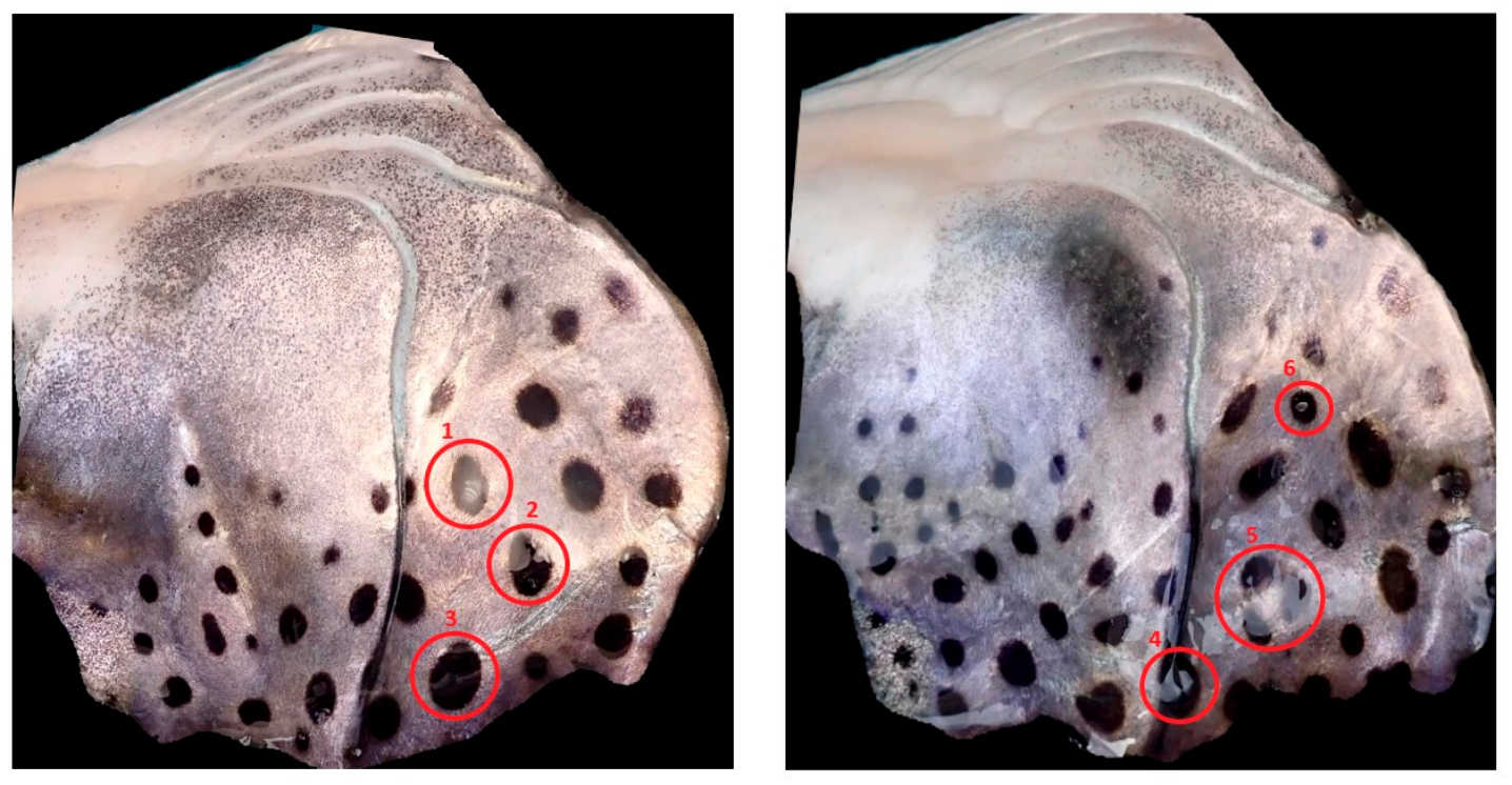
Figure 10. Salmon specimen with spots exhibiting specular highlights (1) and partial (2, 3, 4, and 6) and complete (5) occlusion due to mucus and water droplets.
Fishes 11 00271 g010
Figure 11. (a,b) Pre- and post-stress spot segmentations (along with some false positives; highlighted operculum regions and portion of backgrounds). (c,d) Manually curated and matched spots.
Fishes 11 00271 g011
Figure 12. Individual trajectories for within-fish grayscale changes across day.
Fishes 11 00271 g012
Figure 13. Boxplot distribution of grayscale intensity by day and side.
Fishes 11 00271 g013
Figure 14. Plasma cortisol (% of control mean) in control (n = 8) and stress-treated fish (n = 21). Boxplots show medians and IQRs; points represent individual fish. Cortisol levels were higher in the stress group (Wilcoxon rank-sum test, W = 14, and p < 0.001; *** p < 0.001).
Fishes 11 00271 g014
Figure 15. Distribution and variation in spots grayscale values in control (left) and stressed fish (right). The central tendency and means are also mentioned.
Fishes 11 00271 g015
Figure 16. (Top) For each spot on each fish on each side and day, four nearest neighbors were identified, and directed graphs were constructed. Grayscale differences between each spot and its neighbors were calculated for Days 1 and 2 and utilized in L1 distance computations (0 = identical; 1 = completely different). (Bottom) The boxplots show fish-wise variation in L1 values, with a median trendline indicating central tendency. Sample numbering on x-axis corresponds to the fish specimen sample ID and green triangles highlight the mean value.
Fishes 11 00271 g016
Figure 17. Green background image with all spots included for a fish sample (pre-stress, left side).
Fishes 11 00271 g017
Figure 18. Grayscale with intervals between 0 (black) and 1 (white).
Fishes 11 00271 g018
Figure 19. Scatter plots with fitted regression lines showing the correlation between Observer E and Observer H, and averaged observer grayscale scoring and algorithm-derived grayscale scoring, with Pearson’s r and corresponding p-values indicated.
Fishes 11 00271 g019
Table 1. Training data augmentations during training.
Augmentation TypeUpper Limit Value
Translate: Translates the image horizontally and vertically by a fraction of the image size [0.0–1.0]0.015
Scaling: Scales the image by a gain factor [0–1]0.15
BGR Channels Alteration: Flips the image channels from RGB to BGR with the specified probability [0.0–1.0]0.1
Image Mosaic: Combines four training images into one with the specified probability [0.0–1.0]0.3
Flip Up and Down: Flips the image upside-down with the specified probability [0.0–1.0]0.5
Flip Right and Left: Flips the image left to right with the specified probability [0.0–1.0]0.5
Cutmix: Combines portions of two images with probability [0.0–1.0]0.015
Copy_paste: Copies and pastes objects across images to increase object instances with probability [0.0–1.0]0.0
Shearing: Shearing image randomly between [0°–180°]
Degrees: Rotating image randomly between [0°–180°]
Hue: Hue of the image randomly between [0.0–1.0]0.01
Saturation: Saturation of the image randomly between [0.0–1.0]0.5
Value: Brightness of the image randomly between [0.0–1.0]0.4
Table 2. Salmon operculum segmentation model training and validation metrics.
ModelPrecision (Bbox)Recall (Bbox)Precision (Mask)Recall (Mask)mAP50
(Mask)
mAP50-95
(Mask)
Training0.950.970.950.970.9950.796
Validation0.9981.000.9981.000.990.76
Notes: YOLOv8 precision, recall, and mean average precision with intersection-over-union (IoU) threshold range = [50,95] are computed utilizing bounding boxes and masks associated with the ground truths and predictions. There is only one explicitly mentioned class, i.e., roi.
Table 3. SAM 2.1 averaged losses.
ModeBCE LossIoU LossMask Loss
Training0.0080.16650.0025
Notes: All the losses are normalized in range [0–1] and averaged over total number of training epochs.
Table 4. Percentage change in grayscale pixel intensities per fish and side.
Fish SampleChange Left (%)Change Right (%)
1016.01135.41
1133.1167.19
12 2020.87
1348.985.19
1453.3338.88
15−8.07−0.8
1615.4124.56
1734.706.6
1883.1660.33
19111.18−11.52
2085.510.76
2176.5725.90
2263.79133.33
2345.0764.98
2459.4818.70
2586.50173.17
2657.14−7.69
2776.5385.89
2813.88−3.14
2967.92128.64
30103.548.37
Average54.4646.46
Table 5. Percentage change in grayscale pixel intensity for each fish and side, as assessed manually by the observers.
Fish SampleObserver
(E)
Observer
(H)
Change Left
(%)
Change Right (%)Change Left (%)Change Right (%)
104.5156.0713.44125.44
1145.1496.3416.8059.44
1223.1232.25−5.6631.19
1336.53.4165.47−8.90
1486.541.9532.0137.03
1511.375.2241.660.87
1612.843.0818.324.26
1759.551.117667.64
18 118.7132.8375104.71
1976.90127.270
2066.3614.4737.850
2165.1691.30133.54128.08
2241.24164.7223.3297.76
23N/AN/AN/AN/A
2457.4761.2925.3194.66
25N/AN/AN/AN/A
2640.8496.5565.7672
2786.82235.0856.52110
2836.58−4.5436.6063.20
2959.01028.040
3011316.66133.919.68
Average54.8365.1552.6952.52
Notes: Some of the sample values replaced with N/A were not manually scored by the human observers due to complications in accurately extracting them.
Disclaimer/Publisher’s Note: The statements, opinions and data contained in all publications are solely those of the individual author(s) and contributor(s) and not of MDPI and/or the editor(s). MDPI and/or the editor(s) disclaim responsibility for any injury to people or property resulting from any ideas, methods, instructions or products referred to in the content.