Abstract
This paper describes an approach to determine a fast-charging profile for a lithium-ion battery by utilising a simplified single-particle electrochemical model and direct collocation methods for optimal control. An optimal control problem formulation and a direct solution approach were adopted to address the problem effectively. The results shows that, in some cases, the optimal current profile resembles the current profile in the Constant Current–Constant Voltage charging protocol. Several challenges and knowledge gaps were addressed in this work, including a reformulation of the optimal control problem that utilises direct methods as an alternative to overcome the limitations of indirect methods employed in similar studies. The proposed formulation considers the minimum-time optimal control case, trade-offs between the total charging time, the maximisation of the lithium bulk concentration, and energy efficiency, along with inequality constraints and other factors not previously considered in the literature, which can be helpful in practical applications.
1. Introduction
Green energy research has grown exponentially in the last 20 years [1,2], and one of the most active areas of research that supports green energy and transportation is the technology of rechargeable batteries. The increasing interest in batteries is justified because they possess many attractive features: flexible installation, modularisation, rapid response, and short construction cycles [2]. Fast-charging procedures will play an essential role in achieving the faster deployment of new intermittent renewable energy infrastructure and its interconnection with the electricity grid. Moreover, the development of fast-charging approaches that ensure safety and minimise battery degradation will play a key role in the adoption of electric vehicles, reducing the driver’s waiting time and range anxiety [3].
The Constant Current–Constant Voltage (CC-CV) approach is recognised as one of the most effective methods for charging batteries. The CC-CV charging protocol is favoured for fast-charging applications due to its ability to quickly charge the battery in the CC stage, followed by a controlled charging process in the CV stage. This protocol helps to improve charging efficiency, prevent overcharging, and extend the battery’s lifespan. There are two main stages involved in the CC-CV charging protocol. Initially, the battery is charged with a steady and controlled current until it reaches a pre-determined charge voltage. This stage guarantees that the battery receives an appropriate and consistent current flow. Next, the algorithm moves to the second stage, where a constant voltage is applied to the battery, which continues to slowly charge until the charging time limit or the minimum charging current is reached, which is commonly 3% of the rated current [4]. The CC-CV charging method is particularly well-suited for lithium-ion batteries due to their unique electrochemical characteristics and the requirement to carefully manage the charging process to ensure safety and longevity.
Usually, battery manufacturers provide information sheets with the recommended values for the different phases of the CC-CV protocol [5]. It is well known that elevated temperatures or temperature imbalances can potentially increase the quantity of solid electrolyte interphase growth [6,7], which hinders the performance and longevity of the battery system during operation. Notably, the recommended values are estimated based on laboratory studies, and despite the effort to provide accurate information, these values are not very accurate and the optimal values may change over the lifecycle of the battery. This imprecise estimation may increase costs, reduces the performance and negatively affects other valuable characteristics of the battery pack.
Battery management systems (BMSs) are developed to optimise battery usage, attain safe charging and discharging, and, more significantly, reduce cost. Battery modelling is a necessary task within the BMS and is crucial within many battery control applications [8]. For instance, predicting safe charging in the fastest time is only achievable through advanced battery modelling.
A key problem that drives the research on new and improved battery models is the optimal control of battery charging, which requires the use of a dynamic model of the battery. On the one hand, to reduce the computational time, a good option is to employ a simple electric equivalent circuit model with linear dynamics. On the other hand, a non-linear electrochemical model would be the most accurate representation, as the porous theory models the lithium-ion concentration and other internal parameters. A method by which a transfer function can be calculated from the non-linear model and then converted to a fractional polynomial has been proposed, involving the use of the Padé approximation [2,9,10]. After obtaining the approximation, using the canonical and Jordan forms, the transfer function can be converted to a linear ordinary differential equation system [11,12,13,14,15], which can be used to formulate the battery fast-charging problem as an optimal control problem, using a model derived from electrochemical principles.
In order to address some of the challenges and gaps identified in this research, the optimal control problem presented in reference [3] was reformulated using direct methods, which allowed to overcome the drawbacks of the indirect methods. In the literature, several studies follow a similar methodology for the problem formulation [3,16,17]. However, the existing models do not consider the trade-offs between minimising the total charge time, maximising the lithium bulk concentration, and minimising heat losses. Consideration of these factors may help reduce battery degradation and damage.
One key contribution of this work is to investigate the goal of maximising of the lithium bulk concentration, and how this goal relates to other considerations including charging time and heat losses. An upper bound on the value of the surface concentration has been included in the formulation, as determined by the electrochemical properties of the electrode The incorporation of charging efficiency considerations by including a term in the objective functional to account for heat losses has not yet been tackled in the existing literature. Reducing battery heat losses during charging is crucial as this can help protect the battery from heat damage. Another contribution of this work is the determination of minimum-time charging profiles, which become easy to compute with direct methods for optimal control. All of these considerations affect the charging time and the shape of the input current, and it is understood that the shape of the input current profile has a significant impact on the battery charging process [18]. The challenge for designers is to strike a balance between optimising the total charging time and energy efficiency, while avoiding overheating the battery and considering all relevant constraints.
2. Literature Review
Several papers have addressed the fast-charging problem as an optimal control problem [19,20,21]. Generally, the electrochemical model is the preferred modelling technique to capture the battery’s chemistry. However, its solution can be complex and computationally expensive. The coupled PDEs that describe the electro-chemical processes inside the battery, must be discretised and solved over different domains, which requires ample computation time and memory [22]. Additionally, applying discretisation techniques to convert the PDEs to a system of ordinary differential equations could give rise to peculiar numerical difficulties [23,24], especially if they are stiff systems. Nonetheless, the problem can still be approximated using the technique explained in the following paragraphs.
Various types of battery models are described in the literature [25]. These models can be broadly classified into two categories—model driven and data driven. The model-driven approach makes use of electrochemical relations [26,27,28,29] or employs an equivalent electrical circuit [30,31,32]. Models based on electrochemical relations have the advantage of a physical interpretation, but they can be computationally expensive. Models based on equivalent circuits use electrical elements, such as resistors and capacitors, to represent the behaviour of the battery. These models are computationally less expensive than electrochemical models. Data-driven models, on the other hand, use experimental data to train generic mathematical constructs, such as neural networks [33].
References [34,35] provide a comprehensive evaluation of mathematical models for lithium-ion and nickel-based batteries. The most comprehensive mathematical model widely used in battery simulations is the Doyle–Fuller–Newman model [29,36,37,38], well known in the literature by its acronym DFN ’ [39], is developed using the Maxwell–Stefan equations for the transport of ions in concentrated electrolytes. Fick’s law describes the diffusion of lithium ions in the negative and positive electrodes. The DFN model has been extended and coupled with a temperature model [40,41,42]. It was also further developed to include ageing models [43].
The DFN model is complex due to the presence of seventeen coupled non-linear PDEs and non-linear algebraic equations [22,44]. The model describes the electrochemistry of the battery based on first principles. The input to the model is the applied current density, while the outputs are the terminal voltage, the state of charge, and the state of health. Some authors [45,46,47,48] proposed the use of novel methods to solve the diffusion equations. Moreover, several authors concluded that the DFN model is computationally expensive and unsuitable for the onboard calculation in a battery management system [48]. Researchers have proposed various techniques to simplify the model’s complexity while maintaining accuracy. One approach is to reduce the model dimension. These simplifications target the spherical diffusion process inside the electrodes [49].
A model order reduction by grouping modes with similar eigenvalues is proposed in reference [50]. Also, the work presented in [17] approximated the frequency response of the surface concentration using a Padé approximation. Furthermore, the authors of [51] used the isothermal model based on the first principles of the porous electrode theory to simplify the model. The authors of [50] proposed a model reduction via Galerkin methods with coordinate transformation to solve the spherical diffusion problem. More recently, [52] proposed reducing the DFN complexity in such a way that a simplified model can be used in online applications.
In [53], the complete DFN model was reduced into continuous-form transfer functions. In that paper, the derivation of the transfer function followed the same approach shown in [9], using a rational approximation. In a more recent paper [54], using the simplified model with a Padé truncation and a feedback control strategy, the simplified model outperformed the traditional logic-based approach. In a recent article [52], a divide-and-conquer methodology was used to simplify the DFN further. The model was successfully implemented, and the results showed that the simulations ran many orders of magnitude faster than the state-of-the-art models, making it suitable for online monitoring. Additionally, in reference [55], the authors introduced a framework aimed at simplifying the DFN by mapping its diffusion phases, thermal dynamics, and voltage output to equivalent electric circuit models. The results showed high fidelity at low computation cost.
Several authors proposed the single-particle model with the following corresponding simplifications: firstly, in the geometry (electrodes are considered a single spherical particle); secondly, in the concentration polarisation (no concentration gradients at the boundary); and thirdly, in the movements of Li (the concentration of Li in the electrolyte remains constant) [16,56,57,58,59,60]. The model, derived from the porous electrode theory, simplifies each electrode as a solitary spherical entity. Furthermore, the dynamics of the electrolyte are neglected. More recently, the work presented in reference [35] provides an updated review of the physics-based electrochemical battery models. Furthermore, reference [61] presents an enhanced version of DFN model reduction, named the revised single-particle model. The model approximates the electrochemistry equations using a third-degree polynomial. The outcomes of experiments revealed that the model exhibits high accuracy and is over 30 times faster than the traditional model. However, utilising this model in an optimal control formulation poses several difficulties because of its complexity.
Several variations of the single-particle model exist. For example, the authors of [62] extended the model to use a Kalman filter. In [63], the model defined the volume-average concentration as a state variable, which removes the diffusion PDEs of the lithium concentration in the electrode. Another model simplification was proposed in [56]. The model did not consider the effect of the particle size distribution. In reference [64], using the simplified single-particle model as a baseline and dynamic programming, the optimal charge currents were calculated as a function of the cycle number. In [65], the authors used the single-particle model to solve the minimum-time battery charge using optimal control. Although the results match those presented by other papers that used equivalent circuit models, the methods and procedures used in that article are not sufficiently clear. The simplification proposed in [58], widely adopted due to its accuracy at low values of the rate of discharge and moderate computational costs, is commonly utilised despite its limitation of inaccurate results at high battery current levels. The work described in [66] studied the minimum-time charging problem using bidirectional current pulses and an electric equivalent circuit model, which is less accurate for the estimation of the state of charge than the electrochemical model.
The third-order Padé approximations have been widely used to reduce the complexity of the electrochemistry model [9,11,67,68,69]. In those works, the Padé approximation is applied to the transfer function resulting from combining the evolution of the lithium concentration and the current density [3,70]. In reference [71], the authors performed a runtime test for the third-order Padé model approximation, showing that it presents great superiority in terms of computational complexity. In [72,73,74], similar simplifications were applied to the diffusion partial differential equations using a Padé approximation. However, these papers aimed to simulate lithium batteries rather than formulate optimal control problems.
The implicit optimal control problems formulated for the battery fast-charging problem rely on a set of conditions that the charging current and the state trajectory must satisfy to be considered an optimal solution; those conditions are called the necessary first/second conditions for optimality. The calculus of variations helps find these conditions [75,76,77,78,79]. Two main methods are used to numerically find the optimal trajectory: indirect and direct methods.
Pontryagin’s minimum principle is at the core of indirect methods, which utilise the first-order necessary conditions of optimality. As a result, a two-point boundary value problem is generated. Additionally, the equations can be manipulated analytically, providing a clearer understanding of the solution’s structure. However, indirect methods have a significant drawback: the need to derive the first-order necessary conditions analytically for each problem instance. Moreover, creating an appropriate initial estimate is challenging since it necessitates prior understanding of the control’s switching structure.
Solving optimal control problems using direct methods requires the specification of the type of discretisation approach to be utilised. Discretisation approaches include local approximations, such as the trapezoidal and Hermite–Simpson methods, among others [80,81,82]. Trapezoidal and Hermite–Simpson collocation methods are direct approaches that work by dividing the time interval and approximating the solution within each subinterval using interpolation. The trapezoidal method uses a quadratic interpolating polynomial, while the Hermite–Simpson collocation method approximates the solution using a cubic interpolating polynomial. On the other hand, increasing the number of discretisation points improves the accuracy of the approximation but also increases the computational cost. When using additional discretisation points, the solution can capture more details of the underlying solution, such as sharp transitions or fast variations in the input current. However, doing so requires more computational resources and time. For all the simulations in this work, the maximum relative local error, which measures the accuracy of the approximation of the state variables and is described in [83], was estimated for each candidate solution, and the best solution was chosen for each case to provide the smallest value of this error.
Direct methods for optimal control do not present a general approach to the solution; instead, the numerical algorithm is adjusted for each problem. These algorithms can manage high-dimensional-order systems. Indirect methods offer higher accuracy than direct methods, though the latter are more adaptable and sturdier. Direct methods are designed to easily accommodate bounds on inputs and states, in addition to path and terminal constraints.
3. Battery Fast-Charging Problem
The primary goal of the battery fast-charging problem is to efficiently transition from an initial to a final state of charge while adhering to the problem constraints. Consequently, the battery fast-charging problem has been framed as an optimal control problem. While different battery models have been utilised to formulate and solve this problem, the equivalent circuit model has proven to be particularly effective, offering a reliable approximation [84]. This model produces a system of linear ordinary differential equations that can be solved using well-known numerical methods. In reference [85], the authors developed a closed-form solution of an equivalent circuit model of order one, which was used to show that the bang-and-ride shape of the input current is the best charging policy, considering the objective functional of the optimisation problem as a weighted sum of time-to-charge and heat losses.
Few studies have investigated the battery charging formulated as an optimal control problem. One such study [66] employed a basic equivalent circuit model of order two to determine the optimal equilibrium voltage required for a lithium-ion battery. The authors demonstrated that the problem’s constraints determine whether the minimum-time battery charge solution is a bang-bang or bang-off-bang trajectory as it “switches from one extreme to the other within the bounds” [66]. The same authors reformulated the optimal control problem into the determination of the switching time (switching time refers in this context to the specific moment in time when the input charging current transitions or switches from on to off [86]). The results demonstrated that the model is computationally suitable for embedded applications.
In a more recent publication [87], the authors linearised the single particle model. The resulting model is composed of four linear differential equations. However, the model has limited usability because it made the assumption that the input current has a small amplitude and no direct current component. Linearisation notably simplifies the problem’s analytical solution, but it reduces the solution’s accuracy.
In this work, the battery fast-charging problem is initially formulated according to the methodology described in [3]. The model involves an approximation of the battery cell dynamics using first principles. The objective is to establish a transfer function between the input current and the bulk concentration . Then, by utilising the Laplace transform, the lithium diffusion partial differential equation can be transformed into an ordinary differential equation in the variable s and solved. The concentration dynamics over time that describe the diffusive flow of Li in the negative electrode are represented by a one-dimensional partial differential equation that follows the diffusion model as shown in Equation (1):
which can be transformed into Equation (2):
with Newman boundary conditions:
where is the particle radius of the negative electrode, is the solid diffusion constant of the negative electrode, is the specific interfacial surface area, F is Faraday’s constant, is the electrode current collector specific area, and is the thickness of the negative electrode.
Using Laplace transform applied to (2),
The lithium bulk concentration in the particle is determined by evaluating the solution at . The general solution of Equation (4) with the boundary conditions given in Equation (3) was developed in [9] and is provided in (5):
where is the solid-electrolyte surface concentration. Then, the Padé approximation method can be applied to Equation (5) to obtain a linearised representation of the model [3],
and is given by Equation (7):
where is the volume fraction of filler in the negative electrode and represents, as noted in [72], the mean pore wall movement of lithium ions at the negative current collector. Although, as highlighted in [17], it is unnecessary to estimate the bulk concentration through an additional state variable since it can be directly deduced from (6), the approach in this work follows [8].
As observed in Equation (6), the model conserves, to some extent, the physical meaning of the diffusion process through the presence of and in the resulting transfer function. Additionally, as presented in Equation (7), the transfer function also depends on the geometry of the electrodes. The value for the parameters , , , and for a nickel–manganese–cobalt lithium-ion battery can be obtained from [88].
Assuming zero off-diagonal elements in the system matrix, the final Jordan canonical form is given in Equation (8):
The surface concentration, = is calculated as a linear combination of the states x = , is the row vector defined by the first row of the matrix in Equation (9), while the state represents the bulk concentration.
4. Optimal Control Problem Formulation
Formulating an optimal control problem for fast charging involves the definition of the objective functional, the dynamic equations, the boundary conditions, and any other constraints associated with the problem. The initial step is to define an objective functional representing the optimisation goal. One possibility is to maximise the bulk concentration. The battery dynamics are modelled using the simplified single-particle model, as described in Section 3. The lithium surface concentration needs to be given an upper bound as there is a limit it cannot exceed. The optimal control problem is solved using direct methods and numerical optimisation techniques to find the optimal charging profile, which satisfies the surface concentration constraint, as well as other constraints defined below, while minimising the objective functional.
In mathematical terms, an optimal control problem is typically formulated as follows. Find the final time , the optimal state trajectory , and the control function such that the objective functional J is optimised over the interval , where and are the initial and final time, respectively, and . The variable is the independent variable. The objective functional in Bolza form is given in (10):
where is the end cost, the integral term is known as the running cost, and the scalar function is the integrand. The system is subject to the system state equations (i.e., dynamic constraints)
A set of inequality constraints can be used to express the initial and terminal conditions. These constraints are also known as event constraints:
The problem might also have time-dependent inequality constraints, often called path constraints:
where L and U refer to lower and upper bounds, respectively. The functions , and are defined as per Equation (14)
. There are, in addition, bound constraints on the decision variables as given in Equations (15)–(18)
The formulation of the battery fast-charging problem as an optimal control problem using the third-order Padé approximation of the single-particle model follows. The dynamics of the battery are given in Equation (8). The formulation aims to find an input current profile and a final time to minimise the objective functional, while simultaneously enforcing physical and operational constraints.
The state vector x for the lithium-ion battery cell under the new linear model is:
The meaning and units of the state variables are:
- : state 1 (mol/m)
- : state 2 (mol/m)
- : bulk concentration (mol/m)
On the other hand, the profile of the input current over the time interval needs to be chosen. The letter u is commonly used to represent the control variable such that .
In this study, different formulations of the optimal fast charging problem were analysed, as described in Table 1. It is henceforth assumed that .

Table 1.
Summary of the different formulations of the optimal control problems. Note that the initial time .
4.1. Case 1: Baseline
The model dynamics, constraints and boundaries are obtained from [3]. The authors derived the analytical solution to the battery fast-charging problem using the optimality conditions and Pontryagin’s minimum principle for a fixed final time.
Given the dynamics of the battery as shown in Equation (8), the goal is to determine the final time , the optimal control function and the state trajectory x that maximises the bulk concentration by minimising the objective functional, J:
with the state and input variables bounded as per Equation (20):
where C is the battery rate of discharge (66 Ah), and a single path constraint is given in Equation (21):, which places an upper bound in the surface concentration:
where refers to the first row of the matrix in Equation (9), , and is the maximum surface concentration. The surface concentration cannot go above its maximum value, which depends on the electrochemical characteristics of the electrode, and so 50% of the actual limit has been chosen as the upper bound [3]. The initial state condition is:
4.2. Case 2: Balanced
In [3], the bulk concentration was maximised analytically (indirect method) by minimising the objective functional given in Equation (19).
In contrast, given the dynamics of the battery as shown in Equation (8), in this case the goal is to determine the final time , the optimal control function and the state trajectory, x, that optimises the objective functional:
with the state variables bounded as per Equation (20), a single path constraint given in Equation (21), and the initial condition for the state variables given in Equation (22).
This formulation investigates a balanced optimisation of the bulk concentration and the heat losses, which are given by , where .
4.3. Case 3: Parameterisation of the Objective Functional
The parameterised problem defines different weighting factors in the objective functional. Three sub-cases are summarised in Table 2. The parameters are interpreted as follows: is the relative weight between the final time and the heat losses, is the relative weight between final time and the integral term in the objective functional, and imposes penalties on the internal heat losses. Case 3.1 considers the minimum-time approach, as the final time is being minimised, case 3.2 studies the trade-off between maximising the bulk concentration and reducing heat losses, and case 3.3 investigates the trade-offs between minimising the final time, maximising the bulk concentration, and minimising the heat losses.
Table 2.
Different objective functionals based on the values of the parameters , and for case 3.
Given the dynamics of the battery as shown in Equation (8), the goal is to determine the final time , the optimal control function and the state trajectory, x, that optimise the objective functional:
where is the internal resistance of the cell, the state variables are bounded as per Equation (20), a single path constraint is given in Equation (21), and the initial state condition is given in Equation (22).
This formulation aims to facilitate the investigation of the effects of different terms of the objective functional.
5. Results and Discussion
In each of the following simulation scenarios, the optimal control solver PSOPT is configured to produce the best approximation error possible. PSOPT is an open-source, optimal control solver written in the C++ programming language. The application is described in detail in [89].
5.1. Case 1: Baseline Scenario
The baseline scenario corresponds to the solution of the battery fast-charging problem by maximising the bulk concentration using the third-order Padé approximation of the single-particle model via direct numerical methods. The optimal control trajectory and the are shown in Figure 1. The solution was found analytically using Pontryagin’s minimum principle in [3]. The upper bound on the final time was selected as 450 s. The solution was found using the Chebyshev collocation method with 100 discretisation nodes.
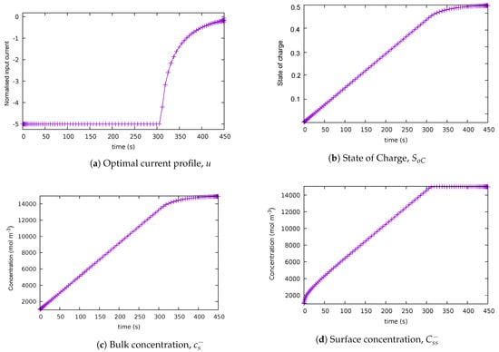
Figure 1.
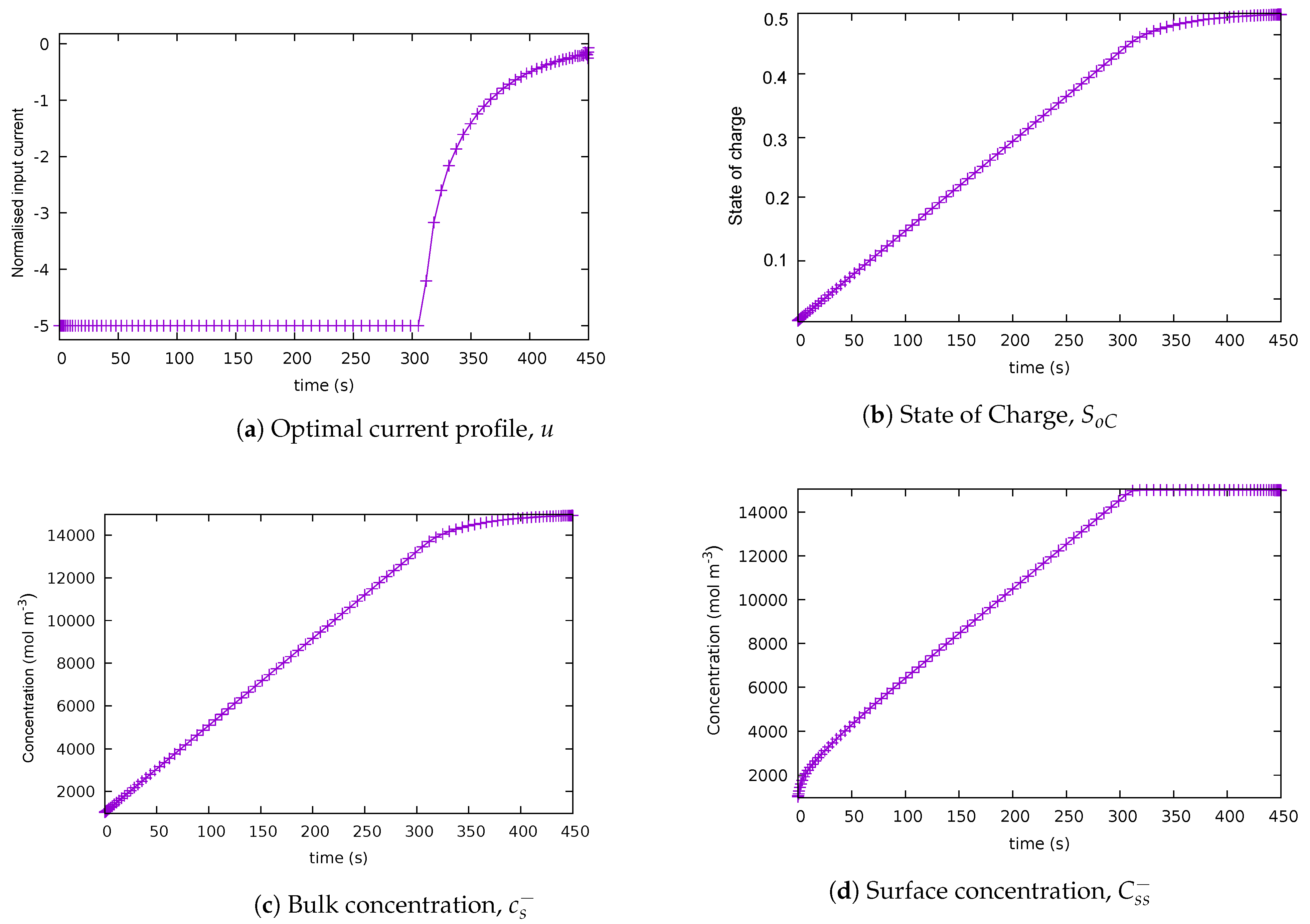
Solution for case 1: baseline scenario. (a) Optimal current profile, u. (b) State of charge . (c) Bulk concentration . (d) Surface concentration .
The quantitative analysis shown in Table 3 confirms that the results obtained in this research are consistent with the findings reported in [3]. Qualitative analysis of the plots in Figure 1 shows that the charging current profile is a bang-and-ride trajectory, in accordance to the results in [3]. Bang-and-ride refers to the input current staying constant at its limit from the start (the bang phase), and then reducing its magnitude from the point where the path-constraint-becomes active (the ride phase). This profile is qualitatively similar to the current profiles that occur when the CC-CV protocol is applied. Note that the path constraint on the surface concentration becomes active at 311 s, thus the switching time between bang and ride was 311 s, while the final time resulted in the upper limit of 450 s. In this case, the initial current was -5C (equivalent to 330 A). What occurs at the switching point is that the dynamics change from a linear ordinary differential equation (ODE) to a linear differential-algebraic equation (DAE) due to the active path constraint. The DAE is of index 1 as the path constraint needs to be differentiated once for the control variable to appear explicitly. As a result, the control variable exhibits a singular arc from the switching point to the final time [83].
Table 3.
Comparison of the results from [3] with the results obtained in this work, in particular for case 1. The switching time refers to the point in time at which the surface concentration reaches its upper limit.
5.2. Case 2: Balanced Scenario
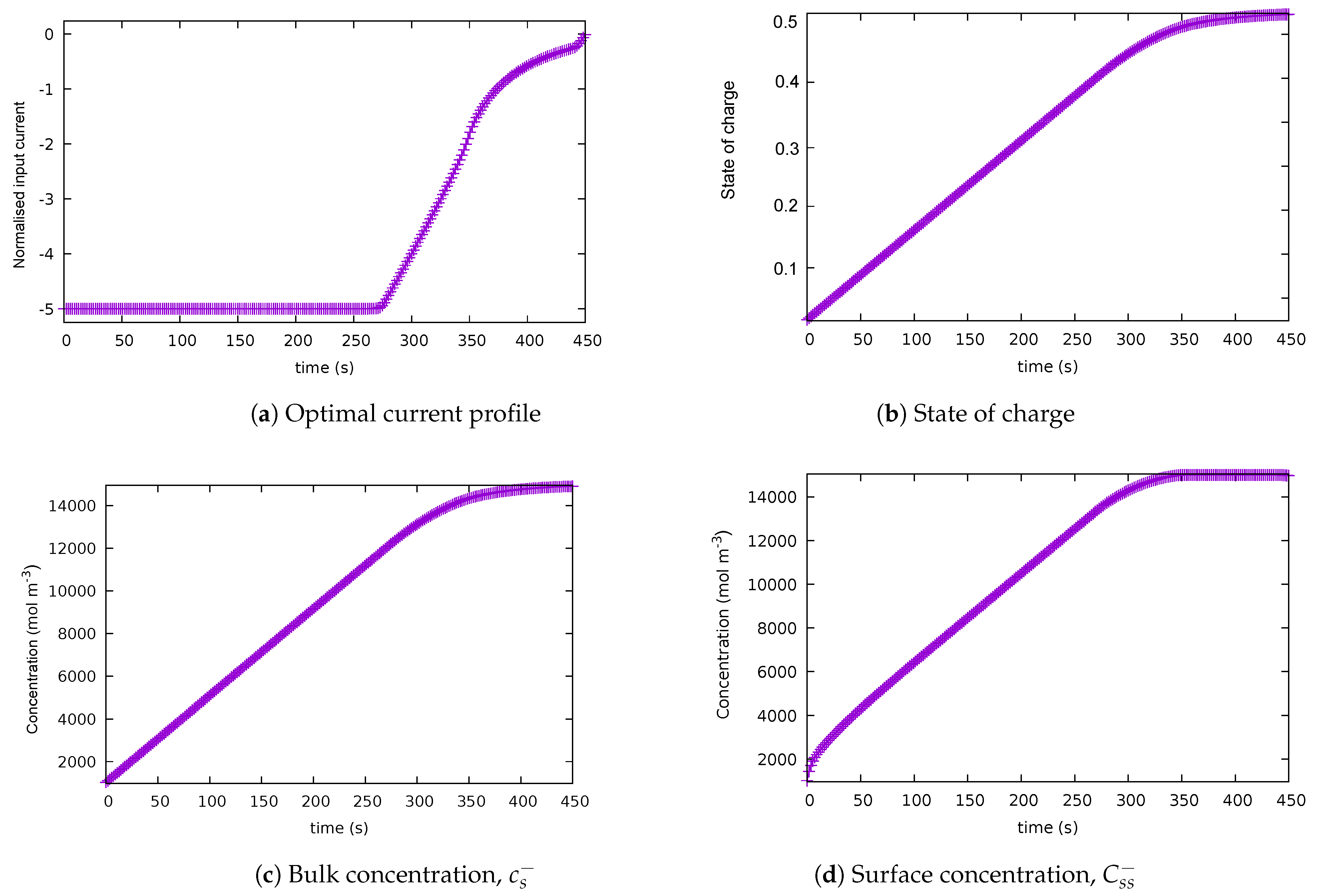
In this case, a term that penalises heat losses was added to the integrand, which originally aimed at maximising the lithium surface concentration. The optimal control trajectory and the state of charge are shown in Figure 2. As can be seen in the figure, the input charging current starts constant at -5C, then it decreases in magnitude after 270 s. Thus, the input current looks like a bang-and-ride trajectory. However, the surface concentration has not reached its upper limit at 270 s; therefore, the path constraint is still inactive at that point in time. The path constraint becomes active at about 350 s, and the surface concentration becomes constant from that point onwards. The state of charge reaches its final value close to the final time of 450 s. The solution shown was found using the trapezoidal collocation method with 250 discretisation nodes.
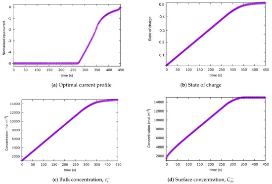
Figure 2.
Solution for case 2: balanced scenario, with the upper bound on the final time = 450 s. (a) Optimal current profile. (b) State of charge. (c) Bulk concentration . (d) Surface concentration
A second experiment was performed using the same problem formulation. On this occasion, the upper bound on the final time was increased from 450 to 550 s. As shown in Figure 3a, the optimal control trajectory starts with a constant value and it decreases in magnitude at around 277 s. Thus, the input current looks like a bang-and-ride trajectory as well. The path constraint associated with the surface concentration becomes active at around 330 s as can be observed from Figure 3c. The state of charge reaches its final value at around 500 s.
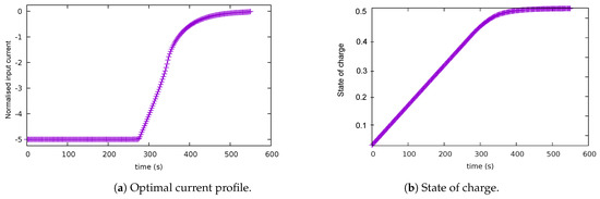
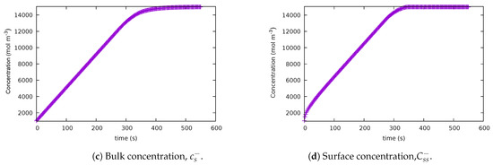
Figure 3.
Solution for case 2: balanced scenario, with the upper bound on the final time = 550 s. (a) Optimal current profile. (b) State of charge. (c) Bulk concentration . (d) Surface concentration
Qualitative analysis of the optimal control trajectory shows that increasing changed the trajectory’s shape. For illustration, the resulting final time, cost (objective functional value), and maximum relative local error is shown in Table 4, for the two different values of the final time.
Table 4.
Cost and maximum relative local error comparison for problem formulation for case 2.
5.3. Case 3: Parameterisation of the Objective Functional
A parametric study was performed to analyse the influence of different terms of the objective functional in the optimal solution. Three parameters were considered: , , and . A detailed description of the cases is shown in Table 2. The solutions in case 3 were found using the Hermite-Simpson collocation method with 150 discretisation nodes.
5.3.1. Case 3.1:
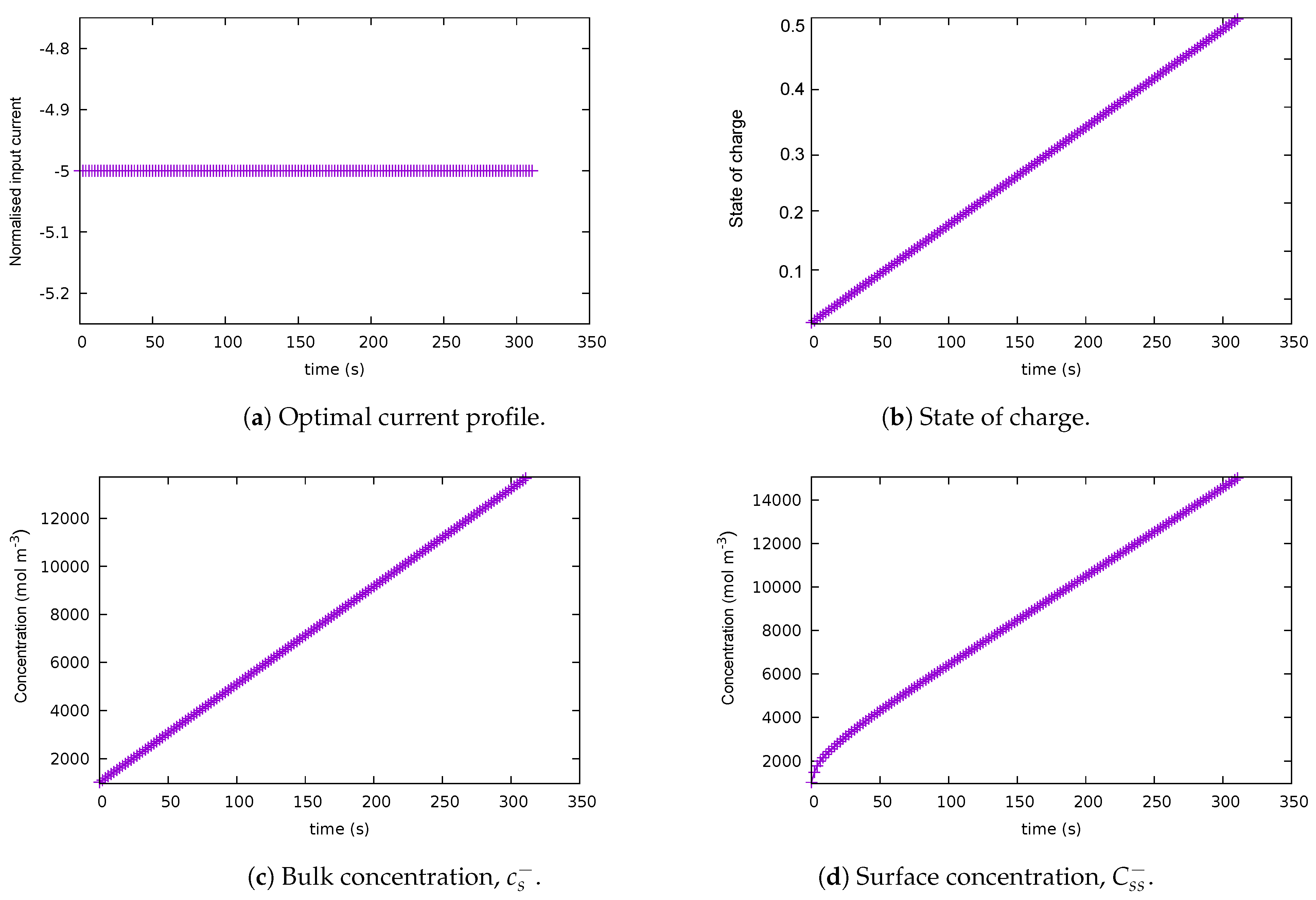
This case exclusively considers minimising the final time based on the parameter = 1 applied to the end cost. Here, the upper bound on the final time was selected as 450 s. All the other parameters ( and ) are not applicable in this case. As observed in Figure 4, the optimal control trajectory is a constant at −5C until the value of s is reached. The path constraint becomes active at the final time, and the state of charge reaches its highest value at the final time.
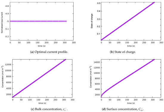
Figure 4.
Solution for case 3.1: = 1. (a) Optimal current profile. (b) State of charge. (c) Bulk concentration . (d) Surface concentration
5.3.2. Case 3.2: , and
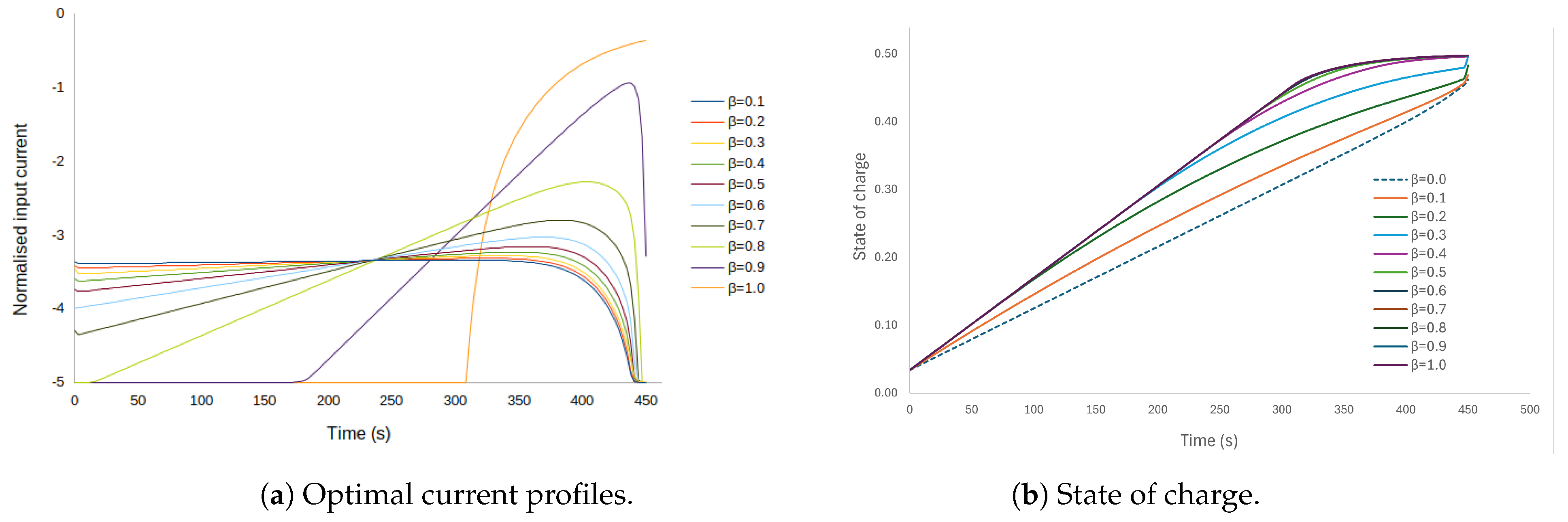
Figure 5 shows the solution when the integrand of the objective function includes a trade-off between the bulk concentration () and the heat loss, which is parameterised by the value of ; with zero end cost. Here, the upper bound on the final time was selected as 450 s. Note that corresponds to the baseline case. As noted in Figure 5a, when the parameter is higher than 0.8, the optimal input current profile has a bang-and-ride shape. For values of lower than 0.8, the optimal input current profile does not resemble a bang-and-ride trajectory. In Figure 5b, the continuous purple line is the state-of-charge trajectory obtained for = 1; the dotted line, which corresponds to the extreme case when , shows that the state of charge reaches its a maximum value at the final time that is lower than the maximum achieved for , while for values of between 0 and 1, the final value of the state of charge increases with increasing values of .
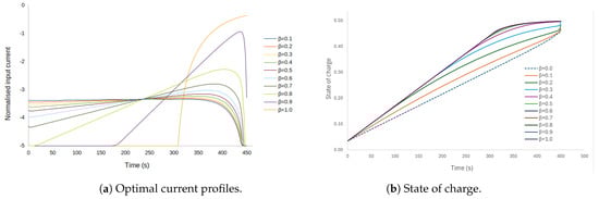
Figure 5.
Different solutions for case 3.2 ( = 0). Charge current profiles for values without the contribution of the final cost. (a) Input current profiles for different values of ; (b) corresponding trajectories of the state of charge for different values of .
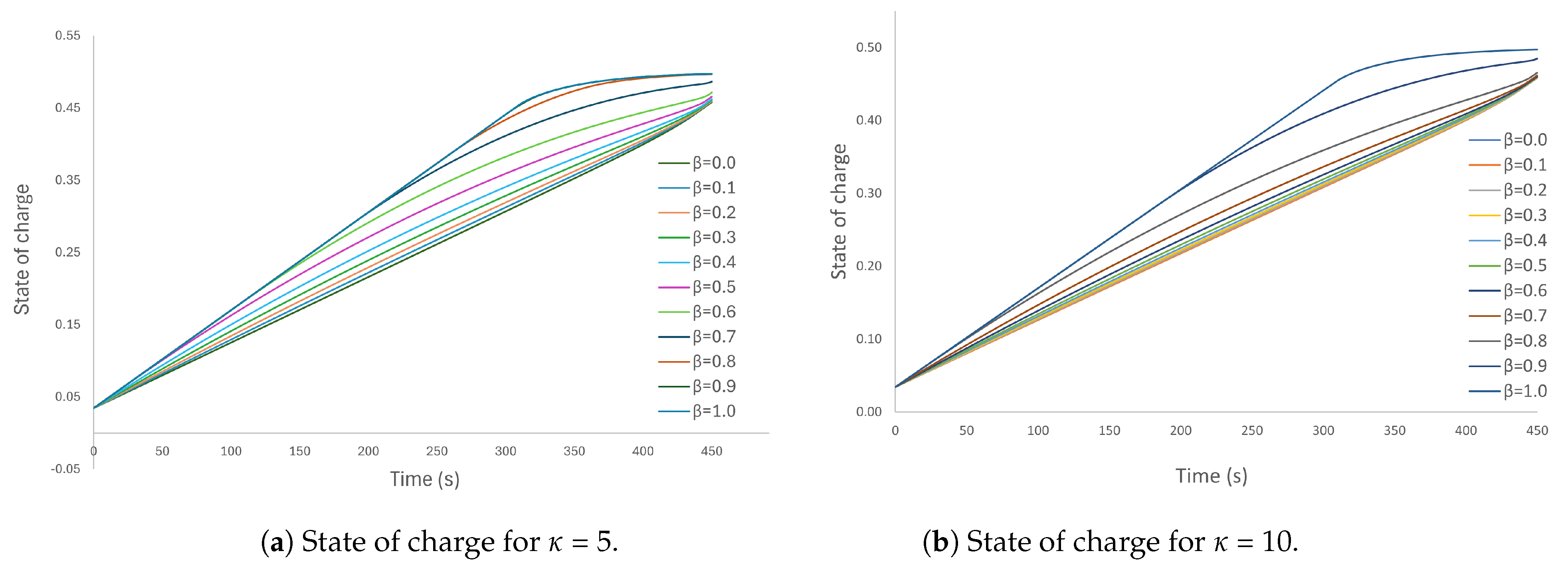
As shown in Figure 6a,b, as the penalty on heat losses increases, the final state of charge is attained more slowly. On the other hand, as the value is increased from 0 for a given value of , the state of charge increases more rapidly towards its final value.
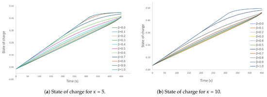
Figure 6.
Solutions for case: 3.2, showing different state of charge for different values of with an additional penalty factor applied to the heat losses. (a) Penalty factor = 5. (b) Penalty factor = 10.
5.3.3. Case 3.3: = 0.8, , = 5
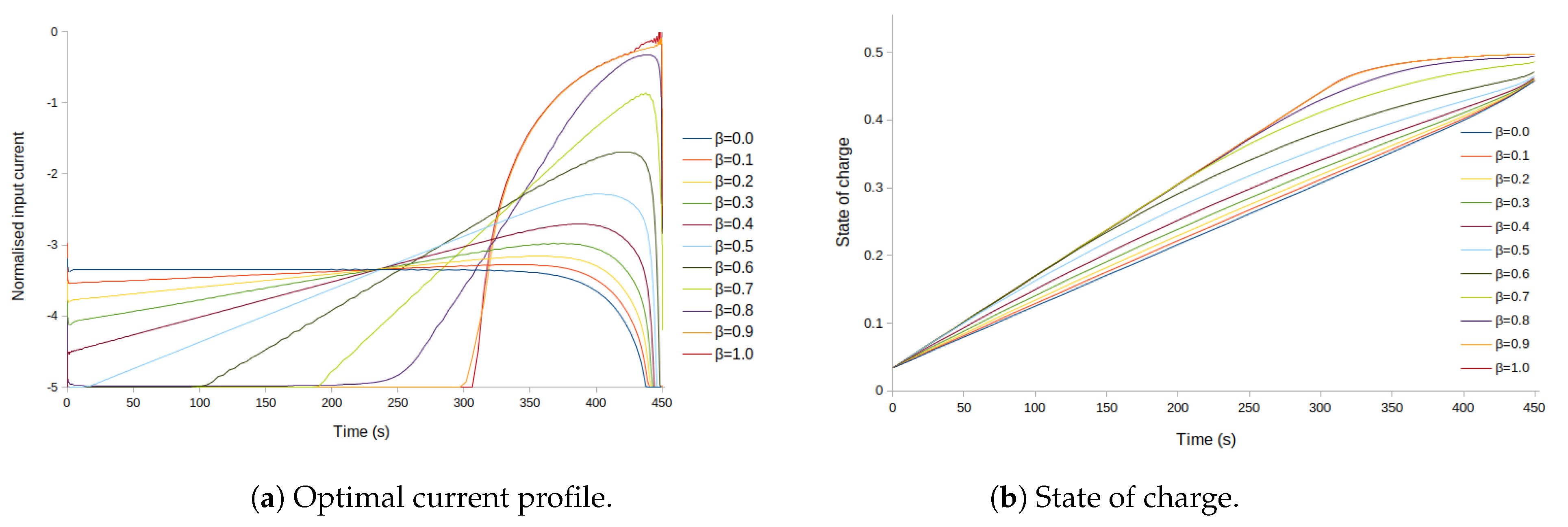
This case considers the trade-offs between minimising charging time, maximising bulk concentration, and minimising heat losses. Here, the upper bound on the final time was selected as 450 s. Figure 7a shows that as the parameter decreases, the similarity of the shape of the input current with the bang-and-ride shape is lost. As expected, reducing the heat losses by penalising them results in a longer charging time.
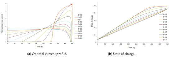
Figure 7.
Solution for case 3.3: State of charge and optimal control trajectory considering the minimisation of the end time, the maximisation of the bulk concentration, and a penalty on the internal losses, for different values of . (a) Input current profile. (b) State of charge profile.
5.4. Analysis of Energy Dissipation in the Parameterised Case
Numerous studies have highlighted the critical role played by heat generation in battery charging [90]. In this paper, heat loss estimation analysis follows the thermal model presented in [91] with simplifications. Specifically, the temperature and the internal resistance are assumed to be constant. The absence of energy transfer between the battery core and the casing simplifies the model as represented by Equation (26).
Given that the control signal is the input charging current, the total heat loss is calculated as follows. If is the total energy dissipated by the internal resistance in kWh, , with in seconds, is the charging current at , is the equivalent internal resistance in , and is defined as ||, then
where is estimated according to the data in [88].
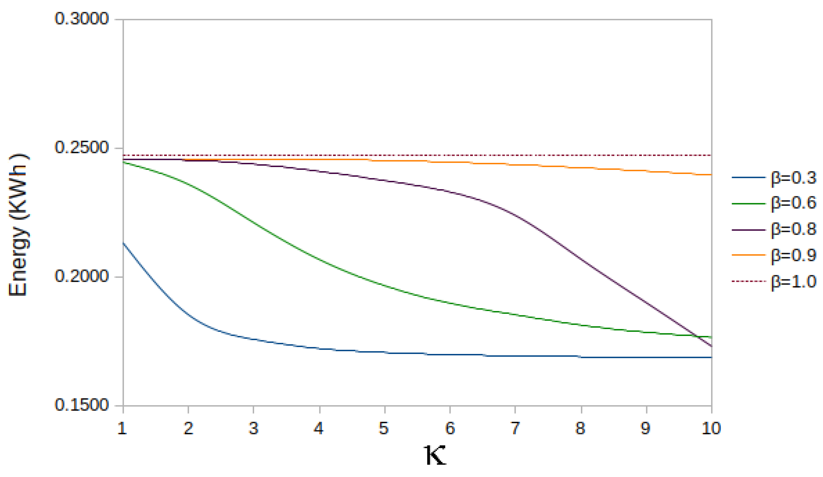
The estimate of the total dissipated energy is shown in Figure 8. The values for the charging current and the simulation time steps used in Equation (26) were obtained from the solutions of case 3.3. The graph shows different contributions of the heat loss in the integrand. As noted, = 1 gives the maximum energy loss of 0.2473 kWh, which is expected as selecting implies that the heat losses are not penalised in the objective functional.
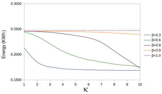
Figure 8.
Comparison of energy dissipation for different contributions in the integrand. The baseline case is shown in orange.
Additionally, the figure illustrates that decreasing leads to a decrease in total heat loss for most values of . For example, when is fixed at 10, setting to 0.9 reduces the total heat losses by 3% (from 0.2473 kWh to 0.2393 kWh). However, reducing to 0.6 results in a 30% reduction in energy loss (from 0.2473 kWh to 0.1764 kWh). The heat loss for = 0.3 yields a 32% reduction. Note that, when reducing below a specific value (0.8), the solution is no longer similar to bang-and-ride trajectory, and that the purple () and green () curves intersect just before . Table 5 provides the values of the energy loss for different values of and .
Table 5.
Estimation of the energy loss in KWh during battery charging for different contributions of lithium () and charging current () in the objective functional.
6. Conclusions
This paper studied the battery fast-charging problem using a simplified model based on electrochemical principles and a direct optimal control approach. The transfer function from the original non-linear dynamics was transformed into a linear state–space form using a third-order Padé approximation, a controllable form, and a Jordan transformation.
In the first phase of the work, the model and optimal control results obtained with our methods were validated using data from the literature for a nickel–manganese–cobalt lithium-ion chemistry. The validation results agreed with the analytical findings reported in [3]. In the second phase, the problem formulation and solution were improved by exploiting the flexibility of direct collocation methods, which allowed to add various terms to the objective functional to study the trade-offs between the minimisation of the charging time, the maximisation of the bulk concentration of lithium, and the minimisation of heat losses.
The direct optimal control approach taken in this work allows for an easy extension to more complex/nonlinear models of the dynamic equations of the battery. Moreover, the approach provides flexibility with regard to the constraints that are required by the problem, and the inclusion of additional terms in the objective functional reflecting additional control objectives.
Author Contributions
Conceptualisation, J.G.-S. and V.B.; methodology, J.G.-S.; software, J.G.-S.; validation, J.G.-S. and V.B.; formal analysis, J.G.-S.; investigation, J.G.-S.; resources, J.G.-S. and V.B.; writing—original draft preparation, J.G.-S.; writing—review and editing, V.B.; visualisation, J.G.-S.; supervision, V.B. All authors have read and agreed to the published version of the manuscript.
Funding
This research received no external funding.
Data Availability Statement
The data presented in this study are available on request from the corresponding author. The data are not publicly available due to the first author’s PhD thesis not having been submitted at the time of publication of this work.
Conflicts of Interest
The authors declare no conflict of interest.
References
- Tan, H.; Li, J.; He, M.; Li, J.; Zhi, D.; Qin, F.; Zhang, C. Global evolution of research on green energy and environmental technologies: A bibliometric study. J. Environ. Manag. 2021, 297, 113382. [Google Scholar] [CrossRef] [PubMed]
- Fan, X.; Liu, B.; Liu, J. Battery Technologies for Grid-Level Large-Scale Electrical Energy Storage. Trans. Tianjin Univ. 2020, 26, 92–103. [Google Scholar] [CrossRef]
- Park, S.; Lee, D.; Ahn, H.J.; Tomlin, C.; Moura, S. Optimal Control of Battery Fast Charging Based-on Pontryagin’s Minimum Principle. In Proceedings of the 59th IEEE Conference on Decision and Control, Jeju, Republic of Korea, 14–18 December 2020. [Google Scholar]
- Liu, H.; Naqvi, I.H.; Li, F.; Liu, C.; Shafiei, N.; Li, Y.; Pecht, M. An analytical model for the CC-CV charge of Li-ion batteries with application to degradation analysis. J. Energy Storage 2020, 29, 101342. [Google Scholar] [CrossRef]
- TrueBluepower. A123-Systems, Nanophosphate High Power Lithium Ion Cell Datasheet. 2022. Available online: https://www.truebluepowerusa.com/pdfs/ANR26650M1-B_ProductFlier.pdf (accessed on 27 February 2023).
- Mohtat, P.; Pannala, S.; Sulzer, V.; Siegel, J.B.; Stefanopoulou, A.G. An Algorithmic Safety VEST for Li-ion Batteries During Fast Charging. IFAC-PapersOnLine 2021, 54, 522–527. [Google Scholar] [CrossRef]
- Carter, R.; Kingston, T.A.; Atkinson, R.W.; Parmananda, M.; Dubarry, M.; Fear, C.; Mukherjee, P.P.; Love, C.T. Directionality of thermal gradients in lithium-ion batteries dictates diverging degradation modes. Cell Rep. Phys. Sci. 2021, 2, 100351. [Google Scholar] [CrossRef]
- Ren, B.; Xie, C.; Sun, X.; Zhang, Q.; Yan, D. Parameter identification of a lithium-ion battery based on the improved recursive least square algorithm. IET Power Electron. 2020, 13, 2531–2537. [Google Scholar] [CrossRef]
- Jacobsen, T.; West, K. Diffusion impedance in planar, cylindrical and spherical symmetry. Electrochim. Acta 1995, 40, 255–262. [Google Scholar] [CrossRef]
- Han, W.; Kalateh Bojdi, Z.; Ahmadi-Asl, S.; Aminataei, A. A New Extended Padé Approximation and Its Application. Adv. Numer. Anal. 2013, 2013, A93–A101. [Google Scholar]
- Shamash, Y. Model reduction using the Routh stability criterion and the Padé approximation technique. Int. J. Control 1975, 21, 475–484. [Google Scholar] [CrossRef]
- Mellodge, P. A Practical Approach to Dynamical Systems for Engineers; Woodhead Publishing: Sawston, UK, 2016. [Google Scholar]
- Chen, T.C. Linear Systems Theory and Design, 3rd ed.; Oxford University Press: Oxford, UK, 1998. [Google Scholar]
- Dorf, R.C.; Bishop, R.H. Modern Control Systems, 14th ed.; Pearson Publishing: London, UK, 2022. [Google Scholar]
- Bernstein, D.S. Matrix Mathematics Theory, Facts, and Formulas with Application to Linear Systems Theory; Oxford Press: Oxford, UK, 2003. [Google Scholar]
- Moon, J. Optimization-Based Reduction and Padeé Approximants for Lithium-Ion Battery Cell Models with Degradation. Master’s Thesis, Texas Tech University, Lubbock, TX, USA, 2022. [Google Scholar]
- Forman, J.C.; Bashash, S.; Stein, J.L.; Fathy, H.K. Reduction of an Electrochemistry-Based Li-Ion Battery Model via Quasi-Linearization and Padé Approximation. J. Electrochem. Soc. 2011, 158, A93–A101. [Google Scholar] [CrossRef]
- Appleton, S.; Fotouhi, A. A Model-Based Battery Charging Optimization Framework for Proper Trade-offs Between Time and Degradation. Automot. Innov. 2023, 6, 204–221. [Google Scholar] [CrossRef]
- Chen, G.J.; Liu, Y.H.; Cheng, S.; Pai, H.Y. A Novel Optimal Charging Algorithm for Lithium-Ion Batteries Based on Model Predictive Control. Energies 2021, 14, 2238. [Google Scholar] [CrossRef]
- Lan, T.; Hu, J.; Kang, Q.; Si, C.; Wang, L.; Wu, Q. Optimal control of an electric vehicle’s charging schedule under electricity markets. Neural Comput. Appl. 2013, 23, 1865–1872. [Google Scholar] [CrossRef]
- Klein, R.; Chaturvedi, N.; Christensen, J.; Ahmed, J.; Findeisen, R.; Kojic, A. Optimal Charging Strategies in Lithium-Ion Battery. In Proceedings of the 2011 American Control Conference, San Francisco, CA, USA, 29 June–1 July 2011; pp. 382–387. [Google Scholar]
- Zou, C.; Kallapur, A.G.; Manzie, C.; Nesic, D. PDE battery model simplification for SOC and SOH estimator design. In Proceedings of the 2015 54th IEEE Conference on Decision and Control (CDC), Osaka, Japan, 15–18 December 2015; pp. 1328–1333. [Google Scholar]
- Stoer, J.; Bulirsch, R. Introduction to Numerical Analysis; Springer: Berlin/Heidelberg, Germany, 1980. [Google Scholar]
- Alt, W.; Schneider, C.; Seydenschwanz, M. Regularization and implicit Euler discretization of linear-quadratic optimal control problems with bang-bang solutions. Appl. Math. Comput. 2016, 287–288, 104–124. [Google Scholar] [CrossRef]
- Plett, G. Battery Management Systems, Volume I: Battery Modeling; Artech House Publishers: Boston, MA, USA, 2015. [Google Scholar]
- Xiong, R.; Li, L.; Li, Z.; Yu, Q.; Mu, H.U. An electrochemical model based degradation state identification method of Lithium-ion battery for all-climate electric vehicles application. Appl. Energy 2018, 219, 264–275. [Google Scholar] [CrossRef]
- Li, X.; Huang, Z.; Tian, J.; Tian, Y. State-of-charge estimation tolerant of battery aging based on a physics-based model and an adaptive cubature Kalman filter. Energies 2021, 2020, 119767. [Google Scholar] [CrossRef]
- Liu, B.; Tang, X.; Gao, F. Joint estimation of battery state-of-charge and state-of-health based on a simplified pseudo-two-dimensional model. Electrochim. Acta 2020, 344, 136098. [Google Scholar] [CrossRef]
- Doyle, C. Design and Simulation of Lithium Rechargeable Batteries. Ph.D. Thesis, University of California, Berkley, CA, USA, 1995. [Google Scholar]
- Thakkar, R.R. Electrical Equivalent Circuit Models of Lithium-ion Battery. In Management and Applications of Energy Storage Devices; Okedu, K.E., Ed.; IntechOpen: Rijeka, India, 2021; Chapter 1. [Google Scholar]
- Cheng, X.; Yao, L.; Xing, Y.; Pecht, M. Novel Parametric Circuit Modeling for Li-Ion Batteries. Energies 2016, 9, 539. [Google Scholar] [CrossRef]
- Zhang, C.; Li, K.; Mcloone, S.; Yang, Z. Battery modelling methods for electric vehicles—A review. In Proceedings of the 2014 European Control Conference (ECC), Strasbourg, France, 24–27 June 2014; pp. 2673–2678. [Google Scholar]
- Zhang, C.; Zhu, Y.; Dong, G.; Wei, J. Data-driven lithium-ion battery states estimation using neural networks and particle filtering. Int. J. Energy Res. 2019, 43, 8230–8241. [Google Scholar] [CrossRef]
- Gomadam, P.M.; Weidner, J.W.; Dougal, R.A.; White, R.E. Mathematical modeling of lithium-ion and nickel battery systems. J. Power Sources 2002, 110, 267–284. [Google Scholar] [CrossRef]
- Planella, F.B.; Ai, W.; Boyce, A.M.; Ghosh, A.; Korotkin, I.; Sahu, S.; Sulzer, V.; Timms, R.; Tranter, T.G.; Zyskin, M.; et al. A continuum of physics-based lithium-ion battery models reviewed. Prog. Energy 2022, 4, 042003. [Google Scholar] [CrossRef]
- Doyle, C.; Fuller, T.F.; Newman, J. Modeling of galvanostatic charge and discharge of the lithium/polymer/insertion cell. J. Electrochem. Soc. 1993, 140, 1526–1533. [Google Scholar] [CrossRef]
- Doyle, C.; Newman, J. The use of mathematical modeling in the design of lithium/polymer battery systems. Electrochim. Acta 1995, 40, 2191–2196. [Google Scholar] [CrossRef]
- Sarkar, S.; Halim, Z.; El-Halwagi, M.; Khan, F. Electrochemical Models: Methods and Applications for Safer Lithium-Ion Battery Operation. J. Electrochem. Soc. 2022, 169. [Google Scholar] [CrossRef]
- Korotkin, I.; Sahu, S.; O’Kane, S.E.J.; Richardson, G.; Foster, J.M. DandeLiion v1: An Extremely Fast Solver for the Newman Model of Lithium-Ion Battery (Dis)charge. J. Electrochem. Soc. 2021, 168, 060544. [Google Scholar] [CrossRef]
- Liu, J.; Pang, H.; Geng, Y.; Chen, K.; Wu, L. Thermal-Coupled Single Particle Modeling and Multi-Objective Stepwise Parameter Identification of Lithium-Ion Batteries Over Different Temperatures. J. Electrochem. Soc. 2023, 170, 060542. [Google Scholar] [CrossRef]
- Schimpe, M.; von Kuepach, M.E.; Naumann, M.; Hesse, H.C.; Smith, K.; Jossen, A. Comprehensive Modeling of Temperature-Dependent Degradation Mechanisms in Lithium Iron Phosphate Batteries. J. Electrochem. Soc. 2018, 165, A181–A193. [Google Scholar] [CrossRef]
- Ramadass, P.; Haran, B.; White, R.; Popov, B.N. Capacity fade of Sony 18,650 cells cycled at elevated temperatures: Part II. Capacity fade analysis. J. Power Sources 2002, 112, 614–620. [Google Scholar] [CrossRef]
- van Beers, J.J. Exploration of the Identifiability and Distinguishability of Battery Degradation Mechanisms in a DFN Model Framework. Master’s Thesis, Eindhoven University of Technology, Eindhoven, The Netherlands, 2023. [Google Scholar]
- Hariharan, K.S.; Tagade, P.; Ramachandran, S. Mathematical Modeling of Lithium Batteries: From Electrochemical Models to State Estimator Algorithms; Springer: Cham, Switzerland, 2018. [Google Scholar]
- Kirkwood, J. Chapter 10—Solving Partial Differential Equations in Spherical Coordinates Using Separation of Variables. In Mathematical Physics with Partial Differential Equations, 2nd ed.; Kirkwood, J., Ed.; Academic Press: Cambridge, MA, USA, 2018; pp. 337–373. [Google Scholar]
- Liu, H.; Yan, J. The Direct Discontinuous Galerkin (DDG) Methods for Diffusion Problems. SIAM J. Numer. Anal. 2009, 47, 675–698. [Google Scholar] [CrossRef]
- de Groen, P.P.N.; van Veldhuizen, M. A Stabilized Galerkin Method for Convection-Diffusion Problems. SIAM J. Sci. Stat. Comput. 1989, 10, 274–297. [Google Scholar] [CrossRef]
- Zhong, L.; Xuan, Y.; Cui, J. Two-grid discontinuous Galerkin method for convection–diffusion–reaction equations. J. Comput. Appl. Math. 2022, 404, 113903. [Google Scholar] [CrossRef]
- Skinner, L.A. Singular Perturbation Theory; Springer: New York, NY, USA, 2011. [Google Scholar]
- Fan, G.; Canova, M. Model Order Reduction of Electrochemical Batteries Using Galerkin Method. In Proceedings of the ASME 2015 5th Annual Dynamic Systems and Control Conference, Columbus, OH, USA, 28–30 October 2015; pp. 1–7. [Google Scholar]
- Dao, T.S.; Vyasarayani, C.P.; McPhee, J. Simplification and order reduction of lithium-ion battery model based on porous-electrode theory. J. Power Sources 2012, 198, 329–337. [Google Scholar] [CrossRef]
- Gu, Y.; Wang, J.; Chen, Y.; Xiao, W.; Deng, Z.; Chen, Q. A simplified electro-chemical lithium-ion battery model applicable for in situ monitoring and online control. Energy 2023, 264, 126192. [Google Scholar] [CrossRef]
- Planden, B.; Lukow, K.; Henshall, P.; Collier, G.; Morrey, D. A computationally informed realisation algorithm for lithium-ion batteries implemented with LiiBRA.jl. J. Energy Storage 2022, 55, 105637. [Google Scholar] [CrossRef]
- Couto, L.D.; Romagnoli, R.; Park, S.; Zhang, D.; Moura, S.J.; Kinnaert, M.; Garone, E. Faster and Healthier Charging of Lithium-Ion Batteries via Constrained Feedback Control. IEEE Trans. Control Syst. Technol. 2022, 30, 1990–2001. [Google Scholar] [CrossRef]
- Biju, N.; Fang, H. BattX: An equivalent circuit model for lithium-ion batteries over broad current ranges. Appl. Energy 2023, 339, 120905. [Google Scholar] [CrossRef]
- Delacourt, C.; Safari, M. Analysis of lithium deinsertion/insertion in LiyFePO4 with a simple mathematical model. Electrochim. Acta 2011, 56, 5222–5229. [Google Scholar] [CrossRef]
- Barbir, F. Chapter Three—Fuel Cell Electrochemistry. In PEM Fuel Cells, 2nd ed.; Barbir, F., Ed.; Academic Press: Boston, MA, USA, 2013; pp. 33–72. [Google Scholar]
- Santhanagopalan, S.; Guo, Q.; Ramadass, P.; White, R.E. Review of models for predicting the cycling performance of lithium ion batteries. J. Power Sources 2006, 156, 620–628. [Google Scholar] [CrossRef]
- Guo, M.; Sikha, G.; Whitea, R.E. Single-Particle Model for a Lithium-Ion Cell: Thermal Behavior. J. Electrochem. Soc. 2010, 158, A122–A132. [Google Scholar] [CrossRef]
- Zhang, D.; Popov, B.; White, R.E. Modelling Lithium Intercalation of a Single Spinel Particle under Potentiodynamic Control. J. Electrochem. Soc. 2000, 147, 831–838. [Google Scholar] [CrossRef]
- Gao, T.; Lu, W. Reduced-order electrochemical models with shape functions for fast, accurate prediction of lithium-ion batteries under high C-rates. Appl. Energy 2024, 353, 121954. [Google Scholar] [CrossRef]
- Di Domenico, D.; Stefanopoulou, A.; Fiengo, G. Lithium-Ion Battery State of Charge and Critical Surface Charge Estimation Using an Electrochemical Model-Based Extended Kalman Filter. J. Dyn. Syst. Meas. Control 2010, 132, 061302. [Google Scholar] [CrossRef]
- Wang, Y.; Fang, H.; Sahinoglu, Z.; Wada, T.; Hara, S. Adaptive Estimation of the State of Charge for Lithium-Ion Batteries: Nonlinear Geometric Observer Approach. IEEE Trans. Control Syst. Technol. 2015, 23, 948–962. [Google Scholar] [CrossRef]
- Rahimian, S.K.; Rayman, S.C.; White, R.E. Maximizing the life of a lithium-Ion cell by optimization of charging rates. J. Electrochem. Soc. 2010, 157, A1302. [Google Scholar] [CrossRef]
- Klein, R.; Chaturvedi, N.A.; Christensen, J.; Ahmed, J.; Findeisen, R.; Kojic, A. Model Order Reduction of Electrochemical Batteries Using Galerkin Method. In Proceedings of the 2011 American Control Conference, San Francisco, CA, USA, 29 June–1 July 2011; pp. 382–387. [Google Scholar]
- Lee, S.; Kim, Y.; Siegel, J.B.; Stefanopoulou, A.G. Optimal control for fast acquisition of equilibrium voltage for Li-ion batteries. J. Energy Storage 2021, 40, 102814. [Google Scholar] [CrossRef]
- Anthony, P. Solving 1-Dimensional diffusion process by Padé approximation. Sci. World J. 2019, 14, 44–47. [Google Scholar]
- Basdebant, J. The Padé approximant and its physical applications. Protein Sci. 1972, 20, 283–331. [Google Scholar]
- Backer, G. Essential of Pade Approximants; Academic Press: London, UK, 1975. [Google Scholar]
- Tran, N.T.; Vilathgamuwa, M.; Farrell, T.; Choi, S.S.; Li, Y.; Teague, J. A Padé Approximate Model of Lithium Ion Batteries. J. Electrochem. Soc. 2018, 165, A1409–A1421. [Google Scholar] [CrossRef]
- Yuan, S.; Jiang, L.; Yin, C.; Wu, H.; Zhang, X. A transfer function type of simplified electrochemical model withmodified boundary conditions and Pade approximation for Li-ion battery. Part 1. lithium concentration estimation. J. Power Sources 2017, 352, 245–257. [Google Scholar] [CrossRef]
- Wu, L.; Liu, K.; Pang, H. Evaluation and observability analysis of an improved reduced-order electrochemical model for lithium-ion battery. Electrochim. Acta 2021, 368, 137604. [Google Scholar] [CrossRef]
- Zhao, Y.; Choe, S. A highly efficient reduced order electrochemical model for a large format LiMn2O4/Carbon polymer battery for real time applications. Electrochim. Acta 2015, 164, 97–107. [Google Scholar] [CrossRef]
- Wu, L.; Pang, H.; Geng, Y.; Liu, X.; Liu, J.; Liu, K. Low-complexity state of charge and anode potential prediction for lithium-ion batteries using a simplified electrochemical model-based observer under variable load condition. Int. J. Energy Res. 2022, 46, 11834–11848. [Google Scholar] [CrossRef]
- Liberzon, D. Calculus of Variations and Optimal Control Theory: A Concise Introduction; Princeton University Press: Princeton, NJ, USA, 2012. [Google Scholar]
- Vinter, R. Optimal Control; Springer Science & Business Media: New York, NY, USA, 2010. [Google Scholar]
- Kirk, D. Optimal Control Theory: An Introduction; Prentice-Hall: Hoboken, NJ, USA, 1970. [Google Scholar]
- Bryson, A.; Ho, Y. Applied Optimal Control-Optimization. Estimation and Control; Taylor & Francis Inc.: Oxon, UK, 1975. [Google Scholar]
- Lao, D.; Zhao, S. Fundamental Theories and Their Applications of the Calculus of Variations; Springer: Beijing, China, 2022. [Google Scholar]
- Lindfield, G.; Penny, J. Numerical Methods Using MATLAB; Oxford Press: Oxford, UK, 2019. [Google Scholar]
- Betts, J. Chapter 1—Issues in the Direct Transcription of Optimal Control Problems to Sparse Nonlinear Programs. In Computational Optimal Control; Bulirsch, R., Kraft, D., Eds.; Birkhauser Verlag: Basel, Switzerland, 1994; Volume 115, pp. 3–17. [Google Scholar]
- Betts, J. Survey of Numerical Methods for Trajectory Optimization. Adv. Astronaut. Sci. 1998, 21, 193–207. [Google Scholar] [CrossRef]
- Betts, J.T. Practical Methods for Optimal Control Using Nonlinear Programming; SIAM: Philadelphia, PA, USA, 2001. [Google Scholar]
- Perez, H.E.; Hu, X.; Dey, S.; Moura, S.J. Optimal Charging of Li-Ion Batteries with Coupled Electro-Thermal-Aging Dynamics. IEEE Trans. Veh. Technol. 2017, 66, 7761–7770. [Google Scholar] [CrossRef]
- Abdollahi, A.; Han, X.; Avvari, G.; Raghunathan, N.; Balasingam, B.; Pattipati, K.; Bar-Shalom, Y. Optimal battery charging, Part I: Minimizing time-to-charge, energy loss, and temperature rise for OCV-resistance battery model. J. Power Sources 2016, 303, 388–398. [Google Scholar] [CrossRef]
- Srinivasan, B.; Bonvin, D.; Palanki, S. Dynamic optimization of batch processes: I. Characterization of the nominal solution. Comput. Chem. Eng. 2003, 27, 185–202. [Google Scholar] [CrossRef]
- Riemann, B.J.C.; Li, J.; Adewuyi, K.; Landers, R.G.; Park, J. Control-Oriented Modeling of Lithium-Ion Batteries. J Dyn. Syst-T ASME 2020, 143, 021002. [Google Scholar] [CrossRef]
- Moura, S. Fast DFN/. 2016. Available online: https://github.com/scott-moura/dfn/blob/master/param/params.m (accessed on 23 November 2023).
- Becerra, V.M. PSOPT Optimal Control Software. 2020. Available online: https://www.psopt.net/ (accessed on 28 November 2022).
- Wang, Z.; Chen, S.; He, X.; Wang, C.; Zhao, D. A multi-factor evaluation method for the thermal runaway risk of lithium-ion batteries. J. Energy Storage 2022, 45, 103767. [Google Scholar] [CrossRef]
- Park, C.; Jaura, A.K. Dynamic Thermal Model of Li-Ion Battery for Predictive Behavior in Hybrid and Fuel Cell Vehicles. SAE Trans. 2003, 112, 1835–1842. [Google Scholar]


Disclaimer/Publisher’s Note: The statements, opinions and data contained in all publications are solely those of the individual author(s) and contributor(s) and not of MDPI and/or the editor(s). MDPI and/or the editor(s) disclaim responsibility for any injury to people or property resulting from any ideas, methods, instructions or products referred to in the content. |
© 2023 by the authors. Licensee MDPI, Basel, Switzerland. This article is an open access article distributed under the terms and conditions of the Creative Commons Attribution (CC BY) license (https://creativecommons.org/licenses/by/4.0/).