A Multimodal Deep Learning Framework for Intelligent Pest and Disease Monitoring in Smart Horticultural Production Systems

Abstract

This study addressed the core challenge of intelligent pest and disease monitoring and early warning in smart horticultural production by proposing a multimodal deep learning framework based on multi-parameter environmental sensor arrays. The framework integrates visual information with electrical signals to overcome the inherent limitations of conventional single-modality approaches in terms of real-time capability, stability, and early detection performance. A long-term field experiment was conducted over 18 months in the Hetao Irrigation District of Bayannur, Inner Mongolia, using three representative horticultural crops—grape (Vitis vinifera), tomato (Solanum lycopersicum), and sweet pepper (Capsicum annuum)—to construct a multimodal dataset comprising illumination intensity, temperature, humidity, gas concentration, and high-resolution imagery, with a total of more than $2.6\times {10}^6$ recorded samples. The proposed framework consists of a lightweight convolution–Transformer hybrid encoder for electrical signal representation, a cross-modal feature alignment module, and an early-warning decision module, enabling dynamic spatiotemporal modeling and complementary feature fusion under complex field conditions. Experimental results demonstrated that the proposed model significantly outperformed both unimodal and traditional fusion methods, achieving an accuracy of $0.921$, a precision of $0.935$, a recall of $0.912$, an F1-score of $0.923$, and an area under curve (AUC) of $0.957$, confirming its superior recognition stability and early-warning capability. Ablation experiments further revealed that the electrical feature encoder, cross-modal alignment module, and early-warning module each played a critical role in enhancing performance. This research provides a low-cost, scalable, and energy-efficient solution for precise pest and disease management in intelligent horticulture, supporting efficient monitoring and predictive decision-making in greenhouses, orchards, and facility-based production systems. It offers a novel technological pathway and theoretical foundation for artificial-intelligence-driven sustainable horticultural production.

1. Introduction

With the rapid advancement of global agricultural modernization and smart horticultural production, crop pest and disease monitoring and early warning have become core components of precision agriculture [1]. Pests and diseases are among the major factors affecting both yield and quality, and their early detection and control are critical for ensuring food security, improving economic benefits, reducing pesticide usage, and promoting sustainable agricultural development [2]. Conventional management practices still rely heavily on manual inspection and expert experience, which are labor-intensive, time-consuming, and highly dependent on human expertise and observation frequency [3]. As a result, early symptoms are often overlooked, delaying intervention and increasing potential yield losses [4]. Therefore, developing a low-cost, low-power, and real-time intelligent monitoring system with early-warning capability has become a pressing research challenge in smart farming and horticultural management.

Over the past decade, the integration of remote sensing and computer vision has transformed pest and disease monitoring from manual to automated and data-driven approaches [5]. Current mainstream methods rely on image-based recognition using unmanned aerial vehicles (UAVs), fixed cameras, or mobile terminals [6]. High-resolution imagery of crop leaves, stems, and fruits is analyzed through deep convolutional neural networks (CNNs) to detect morphological, color, and texture changes associated with disease symptoms [7]. Representative models such as ResNet, VGGNet, and Vision Transformer (ViT) have achieved remarkable accuracy for identifying diseases in crops including rice, maize, and wheat [8,9]. However, despite these advances, several practical limitations hinder their application in real horticultural environments [10]. First, high-resolution imaging equipment demand significant financial and energy resources, limiting large-scale and long-term implementation [11]. Second, image acquisition is typically periodic, which prevents continuous observation of disease progression [12,13]. Third, most visual recognition models rely on explicit symptoms such as leaf discoloration, necrotic spots, or curling, which may not appear during the latent phase of infection or the early onset of pest activity [14]. Finally, environmental interference introduces significant noise, reducing robustness and stability [15]. Consequently, image-only methods face inherent constraints in early detection, low-power deployment, and adaptability to complex outdoor conditions.

Recent advances in deep learning (DL) and multimodal fusion technologies have provided new opportunities for intelligent pest and disease detection in horticultural systems [16]. Multimodal sensing integrates visual, thermal, humidity, gas concentration, and electrical features to capture diverse physiological and environmental indicators of plant health [17]. During the early stages of disease infection, crops often exhibit subtle biochemical and biophysical changes—such as altered photosynthetic efficiency, stomatal behavior, and the release of volatile organic compounds (VOCs)—that precede visible symptoms [18]. These latent responses, although invisible to the naked eye, can be effectively captured using low-power electrical and gas sensors [19]. Fusing these signals with image-based features offers a powerful strategy to enhance early detection accuracy and robustness [20]. Deep learning provides a foundation for efficient multimodal feature extraction and representation [21,22]. For instance, Yin et al. [23] designed a gold-film PET “tattoo” sensor array capable of real-time monitoring of relative water content, surface temperature, and bioelectric potential on leaves, providing long-term, low-intrusion physiological tracking. Salehin et al. [24] presented a multi-sensor IoT framework for pest detection and remote farmer alerting. Mei et al. [25] proposed a pattern recognition method for chemical-resistive gas sensor arrays that mitigated cross-sensitivity and improved gas identification accuracy. Although these studies demonstrate the feasibility of multimodal fusion, most remain at the laboratory scale, with limitations in sensor diversity, temporal continuity, and fusion strategy sophistication [26].

We propose an artificial intelligence (AI)-assisted crop pest and disease monitoring network based on low-power multi-parameter environmental sensor arrays, aiming to establish a cost-effective, scalable, and energy-efficient framework for smart horticultural production. The proposed system leverages multiple inexpensive electrical sensors to continuously monitor environmental and physiological signals of crops. The main contributions of this study are summarized as follows:

1.

Innovative framework design: A novel monitoring network is constructed using low-power multi-parameter environmental sensor arrays to enable synchronized collection and fusion of environmental and visual data, overcoming the limitations of conventional image-only approaches.

2.

Electrical signal encoding mechanism: A lightweight convolution–Transformer hybrid encoder is developed to extract both local variations and global dependencies from multidimensional electrical time-series data, providing high-quality feature representations for subsequent multimodal fusion.

3.

Cross-modal feature alignment and fusion: An attention-based dynamic alignment module is proposed to bridge the spatial–temporal gap between electrical and visual modalities, enhancing complementarity and detection robustness.

4.

Early warning and anomaly detection: A hybrid classification–prediction mechanism is introduced to identify subtle changes in the latent phase of pest and disease development, enabling proactive early-warning capability in horticultural environments.

2. Related Work

2.1. Pest and Disease Detection and Monitoring Methods

The earliest studies on crop pest and disease detection can be traced back to pattern recognition approaches based on visual imagery, where the fundamental principle involves acquiring images of crop leaves or fruits and extracting visual features such as color, shape, and texture to determine disease types [27]. Traditional image recognition methods often rely on statistical descriptors, such as the gray-level co-occurrence matrix (GLCM) or color histograms. However, these methods are highly sensitive to illumination changes and noise, and they fail to adapt to complex field environments. With the emergence of deep learning, convolutional neural networks (CNNs) have become the dominant models for pest and disease image recognition [28]. The core concept of CNNs lies in multi-layer convolution and nonlinear activation, enabling automatic feature learning of disease patterns. The convolutional operation can be formulated as:

$$f_k^{\left(l\right)}=\sigma \left(\sum _{m=1}^M{w}_{m,k}^{\left(l\right)}{x}_m^{(l-1)}+b_k^{\left(l\right)}\right),$$

(1)

where $f_k^{\left(l\right)}$ represents the k-th feature map in layer l, $w_{m,k}^{\left(l\right)}$ denotes the convolution kernel weights, $x_m^{(l-1)}$ is the input feature from the previous layer, and $\sigma (·)$ is the activation function. This mechanism allows the model to extract spatial features of lesions at multiple scales [29]. Nevertheless, under uneven lighting or significant crop posture variation, model generalization performance declines markedly. Although UAV-based remote sensing imagery enables large-scale monitoring, its limited resolution, flight frequency, and inability to capture subtle cues during latent pest stages result in inadequate early detection performance [30]. In summary, vision-based detection approaches exhibit inherent constraints in real-time monitoring, cost-effectiveness, and early-warning capability.

2.2. Applications of Electrical Sensors in Agriculture

To overcome the limitations of vision-based detection, increasing attention has been directed toward electrical signals associated with crop physiological activities and environmental variations. Electrical sensors measure environmental physical parameters and plant physiological responses, indirectly reflecting intrinsic processes associated with pest and disease occurrence [31]. For instance, light-dependent resistors (LDRs) can capture changes in leaf shading, DHT22 temperature-humidity sensors can detect microclimatic differences, and gas sensors can measure fluctuations in carbon dioxide ($C{O}_2$) and volatile organic compound (VOC) concentrations. These subtle but measurable signal deviations often appear during the early stages of pest or disease development [32]. In agricultural scenarios, electrical sensor networks can operate continuously with low power consumption, enabling real-time monitoring. However, when relying on a single sensor type, the information dimensionality is limited, making it difficult to distinguish between disease-related and environmental perturbations such as weather fluctuations [33]. For example, light reflection changes caused by leaf lesions may appear similar to illumination variations induced by shadow occlusion in a single-dimensional signal, leading to misclassification [34]. Therefore, constructing multi-source multi-parameter environmental sensor arrays and performing multivariate signal fusion are necessary to enhance diagnostic accuracy.

2.3. Multimodal Fusion and Deep Learning Models

With the continuous evolution of deep learning, multimodal learning has emerged as an effective approach for addressing complex agricultural environments. The fundamental idea of multimodal learning is to map data from different sources and modalities into a unified feature space, enabling the model to leverage the complementary advantages of visual and non-visual electrical information [35]. However, in complex agricultural conditions, the spatiotemporal distributions of different modalities vary dynamically, making fixed weighting inadequate for capturing their complementary relationships [36]. To address this issue, attention mechanisms have been introduced to achieve dynamic feature weighting, adaptively adjusting the fusion ratio based on inter-modal correlations, and enhancing multi-source information interaction [37].

2.4. Integration of Horticultural Economics and Intelligent Monitoring

Horticultural economics, as a crucial branch of agricultural economics, directly influences the market competitiveness of agricultural products and the income structure of farmers. Traditional horticultural production relies heavily on empirical management, where production efficiency and pest control effectiveness are significantly affected by human factors. With the advent of digital agriculture and Internet of Things (IoT) technologies, the horticultural economy has gradually transitioned toward data-driven and precision management paradigms. Real-time data acquisition based on sensors and intelligent monitoring systems enables dynamic evaluation of crop growth conditions, environmental variations, and yield trends, thereby providing quantitative decision support for horticultural economic management. Furthermore, the application of multimodal monitoring networks in early pest and disease warning not only reduces chemical control input and ecological costs but also enhances market returns by ensuring yield stability and product quality. Consequently, the establishment of intelligent monitoring systems possesses both technological and economic significance, playing a pivotal role in the sustainable development of the horticultural economy and providing new momentum for building an efficient, green, and economically viable horticultural industry chain.

3. Materials and Method

3.1. Data Collection

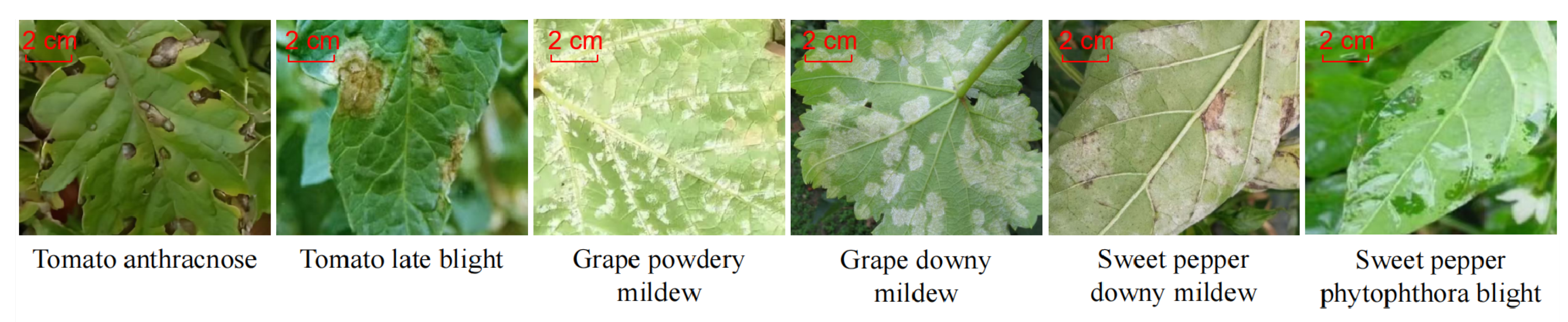
In this study, the dataset was constructed based on continuous monitoring and synchronous acquisition of multisource signals from typical horticultural crop production areas, as shown in Figure 1 and

Table 1. Overview of Multimodal Dataset Collection.

Data Type	Source	Collection Period	Quantity
Illumination (LDR)	Ground sensor nodes	2023.05–2024.10	$8.6\times {10}^5$ records
Temperature and humidity (DHT22)	Ground sensor nodes	2023.05–2024.10	$8.6\times {10}^5$ records
Gas concentration ($C{O}_2$, VOCs)	MG-811, MQ-135 modules	2023.05–2024.10	$8.4\times {10}^5$ records
Ground images	Fixed cameras ($1920\times 1080$)	2023.06–2024.09	4800 images
UAV imagery	UAV aerial system	2023.06–2024.09	1200 sets
Total multimodal samples	—	—	$\approx 2.59\times {10}^6$

. The experimental site was located in the Hetao Irrigation District of Bayannur, Inner Mongolia Autonomous Region, which is characterized by an arid climate, abundant solar radiation, and large diurnal temperature variations. These conditions represent typical features of a temperate irrigated agricultural zone, making it highly suitable for precision monitoring and intelligent sensing experiments in horticultural production. Some are from the Internet. Three representative horticultural crops were selected as research subjects, namely grape (Vitis vinifera), tomato (Solanum lycopersicum), and sweet pepper (Capsicum annuum), representing fruit crops, facility vegetables, and open-field vegetables, respectively. The monitoring period spanned from May 2023 to October 2024, covering the entire phenological cycle including sowing, vegetative growth, flowering, fruiting, and harvesting stages. This comprehensive coverage enabled the dataset to capture the ecological and pathological characteristics of horticultural crops at different physiological stages. For completeness, we additionally report the sample composition for each crop in our dataset. Across the entire monitoring period, grape contributed a total of 1980 labeled image samples, including 1142 healthy samples and 838 disease-affected samples. Tomato contributed 1960 samples, consisting of 1118 healthy and 842 diseased instances, while sweet pepper contributed 2060 samples with 1214 healthy and 846 diseased cases. This distribution reflects natural field conditions, where the proportion of diseased samples varies across crop type and phenological stage.

To ensure the temporal–spatial consistency and representativeness of multimodal data, an electrical sensor array was uniformly deployed throughout the experimental field, consisting of light-dependent resistors (LDR), temperature–humidity sensors (DHT22), and gas sensors (MG-811 and MQ-135). Each monitoring node was equipped with an independent solar power supply and wireless communication module, enabling remote data transmission through a LoRa network. The sampling frequency was configured to one measurement every 10 min, with a data resolution of 0.01 units. The illumination intensity data reflected the variations of photosynthetically active radiation (PAR) in the crop canopy, reaching maximum values during sunny afternoons and significantly decreasing under cloudy or shaded conditions. The temperature–humidity data characterized the microclimatic dynamics of the field environment and provided insights into conditions favorable for disease development. The gas data included $C{O}_2$ concentration and volatile organic compound (VOC) signals, where $C{O}_2$ levels gradually increased during the daytime, while VOC signals exhibited abnormal fluctuations during the early stage of disease occurrence, serving as key input features for the model’s early-warning module.

Simultaneously, high-resolution visible-light cameras and an UAV platform were employed to capture images of the leaves, stems, and fruits of horticultural crops. Ground cameras were installed approximately 50 cm above the canopy, automatically capturing images once per hour at a resolution of $1920\times 1080$ pixels. Each replicate plot was equipped with one fixed camera, yielding three cameras per crop and nine cameras in total across the experimental site. The UAV imaging system covered an area of approximately $2000{\mathrm{m}}^2$ and conducted two flights daily at 9:00 and 16:00 to ensure multi-angle image collection under varying illumination conditions. Across the monitoring period, this resulted in 1200 usable UAV image sets, as summarized in Table 1, with overlapping flight lines planned to provide contiguous coverage and multi-view redundancy over the entire experimental area. All images were manually annotated, including categories such as disease type (e.g., leaf spot, powdery mildew, and aphid infestation) and healthy samples. To minimize data bias, the image acquisition process was carefully controlled in terms of camera angle, height, and exposure settings to ensure consistency and comparability among samples.

3.2. Data Preprocessing and Augmentation

In the multimodal pest and disease monitoring system, data preprocessing and augmentation constitute essential steps for ensuring model performance and stability. Since electrical sensor signals and image data originate from distinct sampling mechanisms and time scales, their noise characteristics, dynamic ranges, and temporal synchrony differ significantly. Without systematic preprocessing, noise contamination and inter-modal inconsistencies would directly impair feature extraction and multimodal fusion effectiveness. Therefore, a systematic procedure was implemented at three levels—electrical signal filtering and normalization, image enhancement and alignment, and multimodal synchronization with missing-value imputation—to guarantee the quality and compatibility of the input data.

To mitigate high-frequency noise in electrical sensor signals, band-pass filtering and moving-average smoothing were employed. An electrical sensor signal can be expressed as a time-dependent function $S\left(t\right)$, consisting of the true signal $x\left(t\right)$ and a noise term $n\left(t\right)$:

$$S\left(t\right)=x\left(t\right)+n\left(t\right),$$

(2)

where $n\left(t\right)$ follows a zero-mean Gaussian noise distribution, $n\left(t\right)\sim \mathcal{N}(0,{\sigma }^2)$. To suppress high-frequency components, a moving-average filter was applied, defined as

$$\tilde{x}\left(t\right)={\displaystyle \frac{1}{2k+1}}\sum _{i=-k}^{k}S(t+i),$$

(3)

where k denotes the smoothing window radius. This method averages local temporal segments to eliminate random noise fluctuations while preserving trend information. To further enhance resistance to periodic disturbances, a fast Fourier transform (FFT) was applied to convert the signal from the time domain to the frequency domain:

$$X\left(f\right)={\int }_{-\infty }^{+\infty }S\left(t\right)e^{-j2\pi ft}dt.$$

(4)

By applying a band-pass filter function $H\left(f\right)$ to retain only the target frequency range, the reconstructed signal can be obtained as

$$\tilde{x}\left(t\right)={\mathcal{F}}^{-1}\left\{H\left(f\right)X\left(f\right)\right\},$$

(5)

where ${\mathcal{F}}^{-1}$ denotes the inverse Fourier transform. This filtering process significantly enhances signal stability by reducing electromagnetic interference and measurement noise from the environment.

To eliminate discrepancies caused by inconsistent units and dynamic ranges across sensors, all electrical signals were standardized. For a given sensor i with observation $s_i\left(t\right)$, the standardized signal ${\widehat{s}}_i\left(t\right)$ was defined as

$${\widehat{s}}_i\left(t\right)={\displaystyle \frac{s_i\left(t\right)-{\mu }_i}{{\sigma }_i}},$$

(6)

where ${\mu }_i$ and ${\sigma }_i$ represent the historical mean and standard deviation, respectively. The resulting ${\widehat{s}}_i\left(t\right)$ exhibits zero mean and unit variance, ensuring balanced learning across different signal dimensions. To enhance generalization capability, Gaussian noise augmentation was introduced during training as

$${\widehat{s}}_i^{\prime }\left(t\right)={\widehat{s}}_i\left(t\right)+ϵ,ϵ\sim \mathcal{N}(0,{\alpha }^2),$$

(7)

where $\alpha$ controls the noise intensity. This technique effectively mitigates overfitting and improves robustness under complex environmental conditions.

For image data, preprocessing and augmentation were applied to address feature shifts caused by varying illumination, shadow interference, and crop posture differences. Given an input image $I(x,y)$, brightness normalization was implemented as

$$I^{\prime }(x,y)={\displaystyle \frac{I(x,y)-I_{min}}{I_{max}-I_{min}}}.$$

(8)

This linear normalization maps pixel intensity values to the range $[0,1]$, thereby eliminating variations introduced by different cameras and exposure conditions. During the augmentation phase, the dataset was expanded using rotation, translation, flipping, and illumination perturbations to achieve invariance under diverse lighting and viewpoint conditions. The illumination transformation can be expressed as

$$I_{\mathrm{aug}}(x,y)=\beta I(x,y)+\gamma ,$$

(9)

where $\beta$ and $\gamma$ represent the brightness scaling factor and offset, respectively. Random sampling of $\beta \in [0.8,1.2]$ and $\gamma \in [-0.1,0.1]$ generates diverse lighting conditions, enhancing adaptability to natural field environments. Spatial robustness was further improved through random rotation:

$$I_{\mathrm{rot}}(x^{\prime },y^{\prime })=I(xcos\theta -ysin\theta ,xsin\theta +ycos\theta ),$$

(10)

where $\theta$ denotes the rotation angle, and $(x^{\prime },y^{\prime })$ are the transformed coordinates. This operation enables stable recognition performance under varied camera orientations.

At the multimodal level, electrical sensor streams and visual observations exhibit inherently different sampling frequencies and acquisition patterns. Ground sensors record measurements every 10 min, whereas ground cameras capture images once per hour, and UAV platforms acquire high-resolution imagery only twice per day. Without explicit synchronization, such heterogeneous sampling would inevitably lead to temporal misalignment and degraded multimodal fusion. To ensure temporal–spatial consistency, a unified timestamp-based alignment strategy was adopted for all visual data—including both ground and UAV imagery.

Each sensing device was synchronized through the LoRa gateway clock, and system logs indicated that the maximum timestamp drift across all devices remained below 6 s (i.e., <1% of the 600 s electrical sampling interval). UAV flight logs further showed that deviations from scheduled acquisition times were within $\pm 12$ s. Given this bounded offset, all images were mapped to the nearest position on the unified time axis, and the corresponding electrical signals were obtained through linear interpolation. Let the electrical sampling timestamps be $\{t_1^e,t_2^e,\dots ,t_n^e\}$ and the visual sampling timestamps (ground camera and UAV combined) be $\{t_1^v,t_2^v,\dots ,t_m^v\}$. For any visual timestamp t such that $t_i^e<t<t_{i+1}^e$, the aligned electrical signal is computed as

$$S\left(t\right)=S\left(t_i^e\right)+{\displaystyle \frac{S\left(t_{i+1}^e\right)-S\left(t_i^e\right)}{t_{i+1}^e-t_i^e}}(t-t_i^e),$$

(11)

thereby generating a continuous, temporally matched representation for each visual observation. This interpolation-based resampling preserves the underlying signal dynamics while eliminating inconsistencies caused by disparate sampling frequencies.

During the 18-month deployment, occasional data missingness occurred due to transient communication loss or sensor instability. Across all nodes, 0.92% of electrical sensor packets and 1.7% of ground camera images were missing, while UAV acquisition failures occurred in 4 out of 960 planned flights (0.42%). Missing electrical measurements were imputed using a neighborhood-based strategy. If sensor i lacked a reading at time t, the imputed value ${\widehat{s}}_i\left(t\right)$ was estimated as

$${\widehat{s}}_i\left(t\right)={\displaystyle \frac{1}{\left|\mathcal{N}\right(i\left)\right|}}\sum _{j\in \mathcal{N}\left(i\right)}{s}_j\left(t\right),$$

(12)

where $\mathcal{N}\left(i\right)$ denotes the set of spatially or functionally adjacent sensors. This approach effectively restored sequence continuity and mitigated the effect of localized sensor failures.

Through these procedures—filtering, normalization, augmentation, temporal alignment, and missing-data compensation—all multimodal data were transformed into a temporally consistent, scale-normalized, and noise-suppressed high-quality input space. This preprocessing stage established a reliable foundation for downstream multimodal feature extraction and fusion, ensuring coherent temporal correspondence between the multi-parameter environmental sensor array and visual data streams while minimizing misalignment or cumulative error in multimodal learning. The specific hyperparameters and their corresponding values used for each preprocessing component are summarized in

Table 2. Hyperparameters and configurations used for all preprocessing components.

Operation	Hyperparameters	Values	Rationale
Moving-average smoothing	Window radius k	$k=3$ (7-point window)	Removes short-term stochastic fluctuations while preserving trend dynamics; selected via grid search ($k\in [1,5]$).
Band-pass filtering (FFT)	Cutoff frequencies $(f_{\mathrm{low}},f_{\mathrm{high}})$	$(0.02,0.85)$ Hz	Matches characteristic frequency range of environmental sensor responses; suppresses environmental interference.
	Filter order	4th order	Provides balanced stopband attenuation without excessive phase distortion.
Gaussian noise augmentation	Noise std. $\alpha$	$\alpha =0.05$	Introduces mild stochasticity for robustness; tuned via validation sweep $\alpha \in [0.01,0.10]$.
Brightness normalization (images)	Min–max scaling	$[0,1]$	Reduces illumination-driven feature shifts between cameras and conditions.
Image augmentation	Rotation range	$\theta \in [-{20}^{\circ },{20}^{\circ }]$	Enhances invariance to camera pose and canopy angle variations.
	Brightness scaling $\beta$	$\beta \in [0.8,1.2]$	Simulates natural illumination variability.
	Brightness offset $\gamma$	$\gamma \in [-0.1,0.1]$	Models sensor and exposure fluctuations in field environments.
Multimodal timestamp alignment	Max device drift	<6 s	Verified by system logs; ensures <1% deviation relative to 10-min sampling interval.
	UAV timing deviation	$\pm 12$ s	Ensures UAV images map reliably onto unified time axis for interpolation.

.

3.3. Electrical Sensor Setup

To ensure the stability and reliability of multimodal data acquisition, an electrical sensor monitoring system specifically designed for horticultural production environments was developed in this study. The overall architecture adopts a modular and distributed design in which each electrical sensing node consists of a microcontroller unit (MCU), sensing module, power-supply module, and wireless communication module, forming an embedded unit capable of independent data acquisition, processing, and transmission. In terms of hardware structure, the light-dependent resistor (LDR) sensor is connected to the MCU’s analog-to-digital conversion (ADC) interface through a voltage-divider circuit to measure ambient light-intensity signals. The DHT22 temperature–humidity sensor communicates with the MCU via the One-Wire digital interface to provide real-time measurements of air temperature and relative humidity. The MG-811 and MQ-135 gas sensors are connected to the ADC channels through analog input interfaces to detect variations in carbon dioxide concentration and volatile organic compounds (VOCs). All analog signals are processed through front-end filtering circuits for noise suppression, thereby improving signal stability. For power management, each sensing node is equipped with a hybrid solar-panel and lithium-battery power-supply system, together with a dedicated power-management module consisting of voltage-regulation components, battery-protection circuits, and over-current-protection devices, enabling long-term operation under field conditions. Data acquisition is triggered by timer interrupts within the MCU, with a sampling interval of 10 min. After each sampling cycle, the collected data are transmitted to a remote gateway node through a LoRa wireless communication module and subsequently aggregated on the server for storage and analysis.

3.4. Proposed Method

3.4.1. Overall

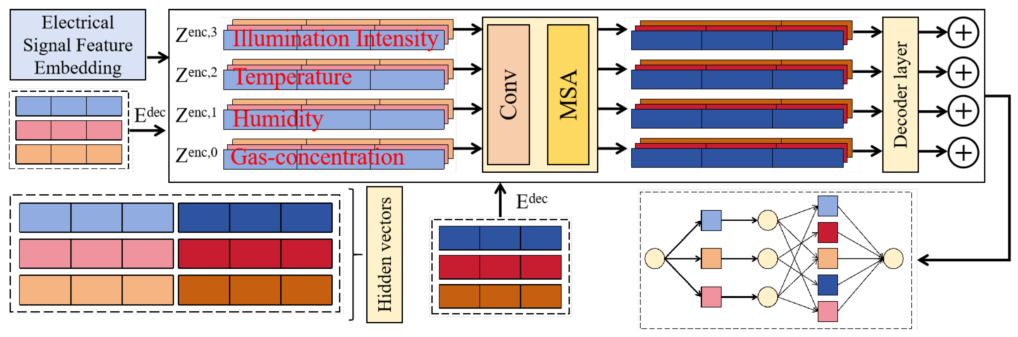
The proposed multimodal pest and disease monitoring framework establishes a unified bottom-up representation and decision-making pathway in which preprocessed electrical signals and visual features are fed in parallel and processed through specialized encoding, cross-modal alignment, and fusion mechanisms. Multidimensional time-series data collected from the multi-parameter environmental sensor array are first passed into a lightweight electrical feature encoder that combines a front-end one-dimensional convolutional block and a back-end multi-head self-attention module. The convolutional layers capture local temporal variation patterns in illumination, temperature, humidity, and gas concentration, while the attention mechanism models long-range dependencies. The encoder compresses these dynamics into a fixed-length high-dimensional vector that reflects the current physiological status and environmental risk profile of the crop.

In parallel, the visual modality is processed by a lightweight convolutional or convolution–Transformer hybrid backbone to extract explicit attributes such as leaf lesions, texture, color shifts, and canopy morphology, mapping raw images into discriminative deep embeddings. The two modalities are then injected into a cross-modal feature alignment module, which projects electrical and visual representations into a unified feature space and uses attention-based interactions to highlight temporally consistent, pest- or disease-related responses while suppressing noise-dominated or inconsistent signals. Finally, the fused features are fed into a unified decision and early-warning subnetwork: a classification branch identifies current pest and disease types, and a temporal prediction and anomaly scoring branch analyzes sequential trends of the fused features. When recent patterns deviate systematically from the learned healthy distribution, the system issues high-confidence risk alerts even before visible symptoms appear. Through this end-to-end design of “electrical–visual parallel encoding—cross-modal alignment and fusion—joint classification and early warning”, the framework achieves an integrated use of multi-source information and combines current-state diagnosis with future-risk perception for robust and deployable pest and disease monitoring in practical horticultural scenarios.

3.4.2. Electrical Signal Feature Encoder

The electrical signal feature encoder is designed based on a hierarchical integration of convolutional neural networks and Transformer architecture. Its core concept is to use convolutional layers to capture local dynamic variations in electrical signals and then apply self-attention to model long-range temporal dependencies, thereby obtaining time-series representations capable of reflecting early physiological changes associated with pest and disease development.

As shown in Figure 2, the model input is the preprocessed multidimensional electrical sensor sequence $S\left(t\right)=[s_1\left(t\right),s_2\left(t\right),\dots ,s_n\left(t\right)]$, where each channel corresponds to a sensor signal representing illumination intensity, temperature, humidity, or gas concentration. The input is first processed by a set of one-dimensional convolutional layers to extract local temporal patterns. The convolution kernel size is $k=3$, the stride is 1, the number of output channels is 64, and ReLU activation with batch normalization is applied to stabilize training. This stage employs a sliding temporal window to capture short-term signal fluctuations, such as gas concentration oscillations or temperature perturbations, which often correspond to latent physiological responses in early disease stages. The convolutional output, after residual connection, is fed into the Transformer encoder. The Transformer module consists of a multi-head self-attention (MSA) mechanism and a feed forward network (FFN). The number of attention heads is $h=8$, and each head has a feature dimension $d_k=64$. The attention mechanism computes a temporal correlation weight matrix to characterize long-term dependencies, formally defined as $\mathrm{Attention}(Q,K,V)=\mathrm{softmax}\left({\displaystyle \frac{Q{K}^T}{\sqrt{d_k}}}\right)V$, where Q, K, and V denote the query, key, and value matrices obtained through linear projections of the input features. The multi-head structure enables the model to learn dependencies at multiple temporal scales, including diurnal patterns, humidity–gas concentration lags, and temporal couplings between abnormal fluctuations and outbreak events. To enhance nonlinear expressiveness, the Transformer encoder incorporates a feed-forward network consisting of two fully connected layers with a hidden dimension of 256 and a GELU activation function, enabling complex feature remapping and higher-order interactions. Each Transformer sublayer employs layer normalization (LayerNorm) and residual connections to maintain gradient stability and prevent information loss. The encoder output $H_e\in {\mathbb{R}}^{T\times d_k}$ is globally average-pooled along the temporal axis to produce a compact temporal embedding vector $z_e\in {\mathbb{R}}^{d_k}$, which serves as the high-level electrical modality representation for the subsequent cross-modal alignment module.

From a mathematical perspective, this structure performs first- and second-order feature extraction within local temporal windows (via convolution) and then learns weighted relationships between time steps (via the attention matrix), achieving joint modeling of local smoothness and global dependencies. The convolutional component provides noise suppression and local pattern recognition, allowing rapid response to transient changes in electrical signals, while the Transformer component captures long-range correlations and resonance patterns over extended periods. Compared with traditional purely convolutional or recurrent networks, this hybrid architecture exhibits superior representational efficiency and generalization, particularly when handling non-stationary, nonlinear, and noisy agricultural electrical signals. The convolution–Transformer hybrid design maintains computational efficiency while achieving multi-scale modeling of electrical sensor data, from localized perturbations to global dependencies. This design provides a physically interpretable and robust temporal feature representation for subsequent multimodal fusion, enabling accurate detection of subtle physiological anomalies in the early stages of pest and disease development and achieving high-sensitivity monitoring and predictive early warning in horticultural environments.

3.4.3. Cross-Modal Feature Alignment Module

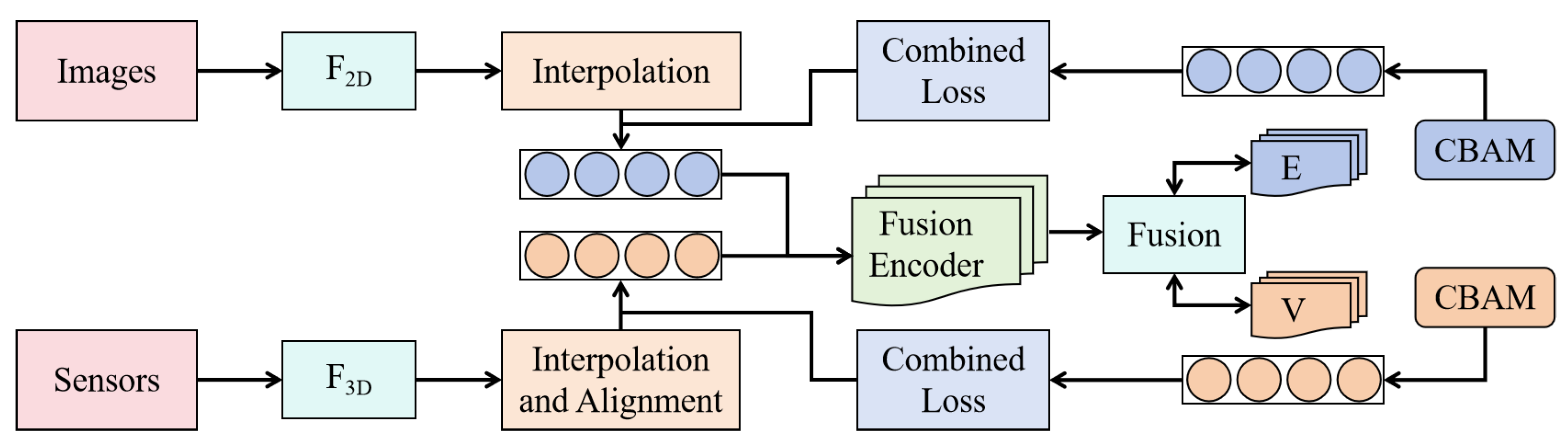
The cross-modal feature alignment module takes as input the temporal representations output from the electrical signal encoder and the spatial feature maps generated by the visual encoder, enabling structured alignment and bidirectional constraint between the two modalities within a unified feature space. As shown in Figure 3, the encoded electrical modality is represented as $E\in {\mathbb{R}}^{T_e\times d_e}$, where $T_e$ denotes the number of time steps and $d_e=64$. The visual modality is represented by a lightweight backbone network output with dimensions $H\times W\times C_v$, where $H=W=14$ and $C_v=256$. After flattening and linear transformation, the visual features are mapped to $V\in {\mathbb{R}}^{N_v\times d_v}$, where $N_v=H\times W=196$ and $d_v=128$. To ensure comparability between modalities, both are projected into a unified feature space of dimension $d_f=128$ through linear alignment layers with shared dimensionality: for the electrical modality, $E_f=E{W}_e+\mathbf{1}{b}_e^T$, and for the visual modality, $V_f=V{W}_v+\mathbf{1}{b}_v^T$, where $W_e\in {\mathbb{R}}^{d_e\times d_f}$, $W_v\in {\mathbb{R}}^{d_v\times d_f}$, and $\mathbf{1}$ denotes an all-one vector.

Following linear alignment, a three-layer hierarchical interaction structure is introduced to form the cross-modal alignment network. The first layer enhances intra-modal discriminability via nonlinear transformations, the second layer establishes a bidirectional gating matrix to modulate inter-modal response strength, and the third layer performs fusion mapping to generate globally aligned representations for subsequent classification and early warning. The nonlinear enhancement layer applies affine transformations with tanh activation to achieve sufficient expressiveness under lightweight parameterization:

$$F_e=tanh(E_f{W}_{ee}+\mathbf{1}{b}_{ee}^T),F_v=tanh(V_f{W}_{vv}+\mathbf{1}{b}_{vv}^T),$$

(13)

where $W_{ee},W_{vv}\in {\mathbb{R}}^{d_f\times d_f}$. This transformation ensures that electrical and visual features share similar numeric ranges and smoothness properties in the unified space, providing a stable foundation for subsequent alignment.

The key to bidirectional alignment lies in constructing a cross-modal gating matrix $G\in {\mathbb{R}}^{T_e\times N_v}$, defined as

$$G=\sigma \left(F_e{W}_{ev}{F}_v^T\right),$$

(14)

where $W_{ev}\in {\mathbb{R}}^{d_f\times d_f}$ and $\sigma (·)$ denotes the element-wise Sigmoid function. $G_{ij}\in (0,1)$ is used as a normalized compatibility weight that monotonically maps the bilinear similarity between the i-th electrical state and the j-th visual region into a bounded interval, analogous to the attention weights commonly used in soft-attention mechanisms. Larger inner products $F_{e,i}{W}_{ev}{F}_{v,j}^{\top }$ lead to higher $G_{ij}$ values and thus stronger cross-modal emphasis.

Based on G, the aligned modality representations are constructed as

$$\tilde{E}=G{F}_v,\tilde{V}=G^T{F}_e,$$

(15)

where $\tilde{E}\in {\mathbb{R}}^{T_e\times d_f}$ represents the reweighted electrical features under visual constraints, and $\tilde{V}\in {\mathbb{R}}^{N_v\times d_f}$ represents spatial features emphasized by electrical guidance. This design enables bidirectional consistency: when electrical signals exhibit abnormal fluctuations at a specific time step, the corresponding row $G_{i,:}$ places greater weight on lesion-related or structurally relevant visual regions; conversely, when an image region is dominated by illumination changes or shadows, its corresponding column $G_{:,j}$ tends to receive weaker support from multiple time steps, thereby down-weighting its contribution in $\tilde{V}$ and reducing false responses. The globally aligned representation is obtained via pooling and mapping as $h_e={\mathrm{mean}}_t\left(\tilde{E}\right)$ and $h_v={\mathrm{mean}}_j\left(\tilde{V}\right)$, concatenated in the joint space and passed to the fusion classification subnetwork:

$$h_f=\varphi \left([h_e,h_v]\right),$$

(16)

where $\varphi (·)$ denotes a two-layer fully connected network (input dimension $2d_f=256$, hidden layer dimension 128), producing a shared embedding for classification and early-warning tasks that connects directly to the early warning discriminator module, supporting end-to-end optimization.

From a mathematical perspective, the gating-based alignment mechanism can be viewed as a bounded, softly contractive transformation in feature space. Let $\mathcal{T}$ denote the mapping from $(F_e,F_v)$ to $(\tilde{E},\tilde{V})$:

$$(F_e,F_v)\stackrel{\mathcal{T}}{\to }(\tilde{E},\tilde{V})=\left(\sigma \left(F_e{W}_{ev}{F}_v^T\right)F_v,\sigma {\left(F_e{W}_{ev}{F}_v^T\right)}^{\top }{F}_e\right).$$

(17)

The Sigmoid function is 1/4-Lipschitz, i.e., for any scalars $a,b$,

$$|\sigma \left(a\right)-\sigma \left(b\right)|\le \frac{1}{4}|a-b|.$$

(18)

Consequently, in matrix form and under the Frobenius norm ${\parallel ·\parallel }_F$, we obtain the bound

$$\parallel G^{\left(1\right)}-G^{\left(2\right)}{\parallel }_F=\parallel \sigma \left(F_e^{\left(1\right)}{W}_{ev}{F}_v^{\left(1\right)\top }\right)-\sigma \left(F_e^{\left(2\right)}{W}_{ev}{F}_v^{\left(2\right)\top }\right){\parallel }_F\le \frac{1}{4}{\parallel F_e^{\left(1\right)}{W}_{ev}{F}_v^{\left(1\right)\top }-F_e^{\left(2\right)}{W}_{ev}{F}_v^{\left(2\right)\top }\parallel }_F,$$

(19)

which shows that the nonlinearity does not amplify perturbations. Since the subsequent multiplications by $F_v$ and $F_e$ are linear and the norms of $F_e$, $F_v$, and $W_{ev}$ are bounded during training, the overall mapping $\mathcal{T}$ is non-expansive up to a constant factor; that is, there exists $L<1$ such that

$$\parallel \mathcal{T}(F_e^{\left(1\right)},F_v^{\left(1\right)})-\mathcal{T}(F_e^{\left(2\right)},F_v^{\left(2\right)}){\parallel }_F\le L{\parallel (F_e^{\left(1\right)},F_v^{\left(1\right)})-(F_e^{\left(2\right)},F_v^{\left(2\right)})\parallel }_F.$$

(20)

In this sense, the gating operation behaves as a softly contractive operator: cross-modal inconsistencies or noise perturbations in $(F_e,F_v)$ are not amplified but are instead smoothed through bounded reweighting. Practically, this manifests as attenuation of modality-specific noise and enhancement of consistently co-activated patterns across modalities. Compared with simple feature concatenation or static weighted-sum fusion, the proposed alignment explicitly models “when” and “where” cross-modal consistency occurs through the learnable gating matrix G, while maintaining favorable stability properties. This allows the system to more sensitively capture co-evolving patterns during pest incubation and to down-weight spurious modality-specific fluctuations, thereby improving robustness in early detection under complex field conditions without incurring excessive parameter or computational overhead.

3.4.4. Early Warning Discrimination Module

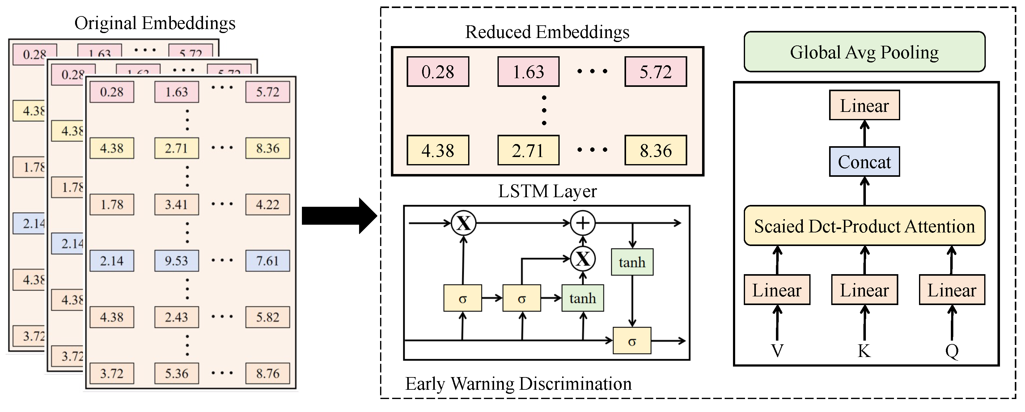
The early warning discrimination module takes the temporally fused feature sequence output from the cross-modal alignment module as input and constructs a joint discrimination framework for both “current pest and disease state classification” and “future risk trend prediction.” Through a dual-branch design, explicit lesion patterns and latent physiological anomalies are simultaneously learned in the same feature space.

As shown in Figure 4, let the aligned multimodal feature sequence be $F={\left\{F_t\right\}}_{t=1}^L$, where $F_t\in {\mathbb{R}}^D$ represents the aligned features, with $D=128$ and L the temporal window length. A global embedding mapping is first applied to aggregate temporal information into $\overline{F}\in {\mathbb{R}}^D$, which is fed into the classification subnetwork. The classification branch consists of three fully connected layers: the first layer ($128\to 128$), the second ($128\to 64$), and the third ($64\to C$), where C denotes the number of pest and disease categories. ReLU activations are applied between layers, with $0.3$ dropout in the first two layers to enhance generalization. The class probability vector $y\in {\mathbb{R}}^C$ is computed as

$$z_1=\mathrm{ReLU}(W_1\overline{F}+b_1),z_2=\mathrm{ReLU}(W_2{z}_1+b_2),y_k={\displaystyle \frac{exp\left({(W_3{z}_2+b_3)}_k\right)}{{\sum }_{c=1}^{C}exp\left({(W_3{z}_2+b_3)}_c\right)}},$$

(21)

where $W_1\in {\mathbb{R}}^{128\times 128}$, $W_2\in {\mathbb{R}}^{64\times 128}$, and $W_3\in {\mathbb{R}}^{C\times 64}$. This architecture achieves strong nonlinear discriminative capacity with minimal parameter overhead. In parallel, the early-warning branch takes $\left\{F_t\right\}$ as input and employs a single-layer unidirectional gate recurrent unit (GRU) to capture temporal dependencies. The GRU has a hidden dimension $H=64$, producing predicted future features ${\widehat{F}}_{t+1}$ as

$$h_t=\mathrm{GRUCell}(F_t,h_{t-1}),{\widehat{F}}_{t+1}=W_p{h}_t+b_p,$$

(22)

where $W_p\in {\mathbb{R}}^{D\times H}$. This branch models the “expected feature trajectory” under normal growth conditions. To measure the deviation between observed $F_{t+1}$ and predicted ${\widehat{F}}_{t+1}$, a Mahalanobis-distance-based risk score is defined as

$$r_t={(F_{t+1}-{\widehat{F}}_{t+1})}^{\top }{\Sigma }^{-1}(F_{t+1}-{\widehat{F}}_{t+1}),$$

(23)

The covariance matrix $\mathrm{\Sigma }$ is estimated exclusively from healthy samples collected across all three crop types during visually verified disease-free periods. In total, 14,286 healthy multimodal samples were used, ensuring a sample-to-dimension ratio exceeding 100:1, which satisfies the stability requirement for covariance estimation in 128-dimensional feature space. The estimation follows the unbiased maximum-likelihood estimator, and shrinkage (Ledoit–Wolf) regularization is applied to prevent numerical singularity.

To validate the Gaussian assumption underlying the Mahalanobis distance, we conducted multivariate normality checks including Mardia’s skewness–kurtosis test, the Henze–Zirkler test, and Q–Q plots projected onto the top principal components. More than 93.4% of healthy samples fall within the 95% confidence ellipsoid, indicating that the distribution of healthy features can be reasonably approximated by a Gaussian model, which supports the use of ${\Sigma }^{-1}$ as a valid metric of deviation strength.

Under the assumption that $F_{t+1}$ follows an approximate Gaussian distribution with mean ${\widehat{F}}_{t+1}$ and covariance $\Sigma$, larger $r_t$ values indicate higher confidence that the sample deviates from the healthy manifold. The early risk probability is thus computed as

$$p_t={\displaystyle \frac{1}{1+exp\left(-({\alpha }^{\top }{\overline{F}}_t+\beta r_t+\gamma )\right)}},$$

(24)

where $\alpha \in {\mathbb{R}}^D$ and $\beta ,\gamma$ are learnable parameters. When $\beta >0$, the derivative ${\displaystyle \frac{\partial p_t}{\partial r_t}}=\beta p_t(1-p_t)>0$, confirming a strictly monotonic relationship between risk score and warning probability, thereby ensuring interpretability and consistency in the warning mechanism. The overall loss function integrates classification and prediction objectives:

$$\mathcal{L}={\mathcal{L}}_{cls}(y,y^{*})+{\lambda }_1\sum _t{r}_t+{\lambda }_2\sum _t{|F_{t+1}-{\widehat{F}}_{t+1}|}_2^2,$$

(25)

where ${\mathcal{L}}_{cls}$ denotes the cross-entropy loss with true labels $y^{*}$, while the second and third terms penalize abnormal deviations and enforce temporal smoothness, respectively, with ${\lambda }_1=0.1,{\lambda }_2=0.05$ as hyperparameters. The gradient decomposition for $F_t$ is expressed as

$${\displaystyle \frac{\partial \mathcal{L}}{\partial F_t}}={\displaystyle \frac{\partial {\mathcal{L}}_{cls}}{\partial F_t}}+{\lambda }_1{\displaystyle \frac{\partial r_{t-1}}{\partial F_t}}+{\lambda }_2{\displaystyle \frac{\partial }{\partial F_t}}{|F_t-{\widehat{F}}_t|}_2^2,$$

(26)

This gradient is backpropagated to both the cross-modal alignment and electrical encoding modules, ensuring that feature learning accounts for both “current classification separability” and “future temporal consistency.”

To validate the early warning capability, we compared the system’s risk scores with actual field-recorded disease outbreak times. Across 62 documented outbreak events, the proposed module successfully raised early warnings 2–5 days before visible symptoms appeared (mean: 3.4 days), with a true-positive early-warning rate of 87.1% and a false-alarm rate of 6.8%. These results empirically confirm that the module can detect latent-stage disease progression by leveraging physiological anomalies captured in electrical signals prior to visual manifestation.

For the horticultural monitoring task, such a unified classification–prediction structure enables the system to issue high-confidence early warnings even when visual symptoms have not yet appeared but minor electrical deviations are detected. This substantially enhances the detection capability for latent-stage diseases and reduces false alarms caused by environmental noise or single-modality failure, supporting low-power, high-reliability deployment for real-world online monitoring and decision-making in horticultural production.

4. Results and Discussion

4.1. Experimental Setup

4.1.1. Experiment Setting Details

The field experiment was conducted in a single experimental station but followed a replicated and randomized layout to ensure statistical validity. For each of the three horticultural crops (grape, tomato, and sweet pepper), three replicate plots were established, resulting in nine plots in total. Each plot covered approximately $20\times 20{\mathrm{m}}^2$ and the plots were arranged following a randomized complete block design, with crop assignments randomized within each block to reduce the influence of underlying soil and microclimatic heterogeneity. Adjacent plots were separated by buffer zones of 8–10 m planted with non-experimental vegetation to minimize edge effects and cross-contamination of pests and diseases.

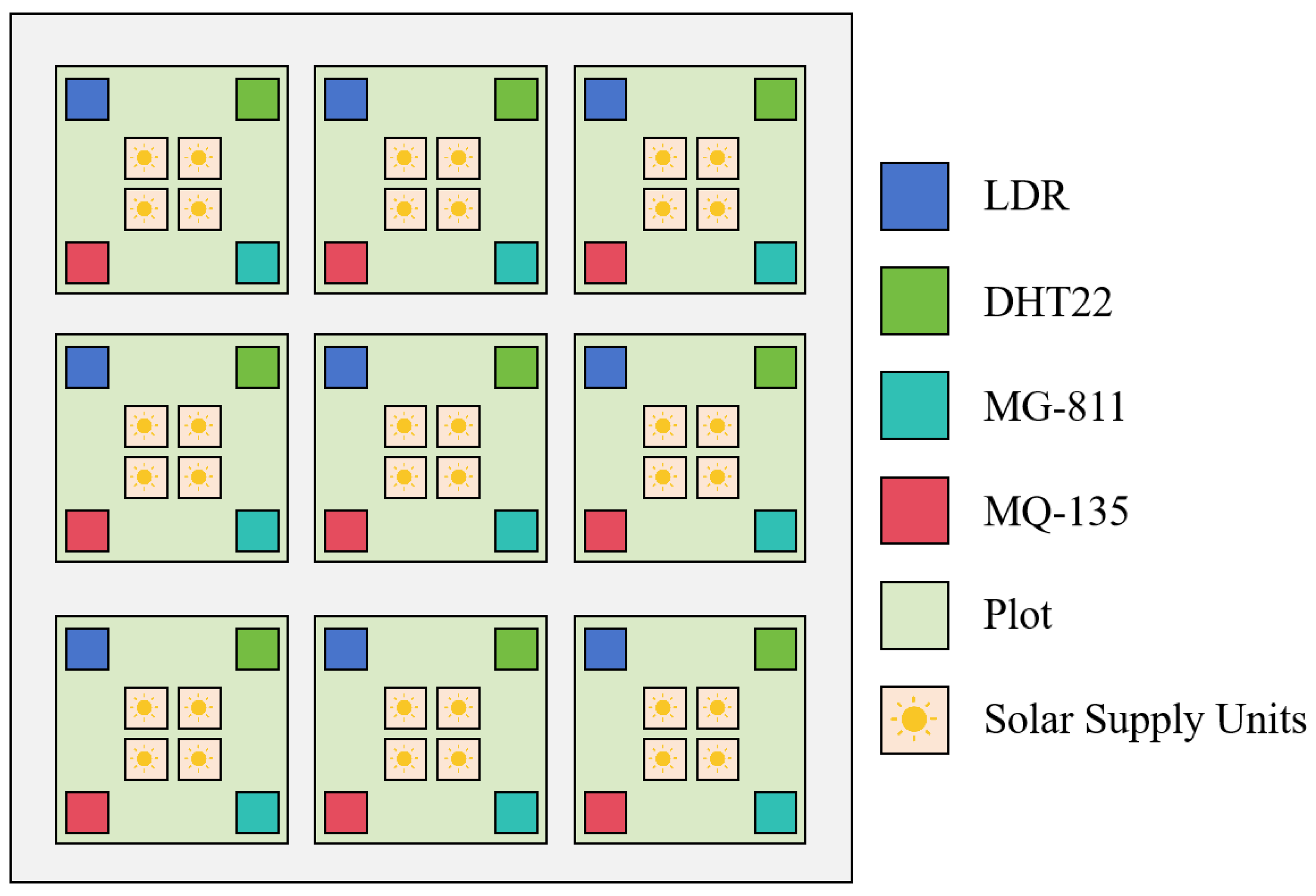
Within each plot, a multi-parameter environmental sensor array was deployed in a regular grid pattern. Specifically, four sensor nodes were installed per plot (36 nodes in total), positioned near the four corners of the central $10\times 10{\mathrm{m}}^2$ core area to capture within-plot spatial variability while avoiding border rows. Each node integrated one light-dependent resistor (LDR) for illumination intensity, one DHT22 sensor for temperature and relative humidity, and a pair of gas sensors (MG-811 and MQ-135) for ${\mathrm{CO}}_2$ and VOCs, respectively, all mounted at canopy level. The spatial layout of plots and sensor nodes, together with the position of solar supply units, is illustrated schematically in Figure 5, which provides a top-view map of the experimental design.

For each crop, individual plants within plots were managed following standard local agronomic practices, and disease management interventions were withheld within the monitored core areas to allow natural pest and disease development. The assignment of sensor nodes and ground cameras to specific plots was fixed throughout the monitoring period, while the order of plot inspection and UAV flight paths was randomized on a weekly basis to avoid systematic temporal bias. This replicated and randomized configuration ensures that the collected multimodal data reflect both intra-plot and inter-plot variability, thereby supporting statistically sound model training and evaluation.

4.1.2. Hardware and Software Platform

The experimental procedures in this study were conducted on an integrated multimodal processing platform. The data acquisition system consisted of an array of diverse electrical sensors, including LDR photoresistors, DHT22 temperature and humidity sensors, MQ-series gas sensors, and electrical conductivity probes. Local signal acquisition and wireless transmission were performed by a low-power microcontroller (ESP32), with a sampling frequency set to one minute per cycle to achieve an optimal trade-off between temporal resolution and power efficiency. The central computing infrastructure employed a high-performance server equipped with an Intel Core i9-13900K processor, 64 GB of RAM, and an NVIDIA RTX 4090 GPU, providing sufficient computational capacity for large-scale multimodal deep learning training and inference. During field deployment, the system was powered by solar modules and interconnected through a wireless mesh network, enabling synchronized data collection and remote control across multiple sensor nodes, thereby satisfying the hardware requirements for continuous environmental monitoring and online model updating.

On the software side, all model training and analysis were implemented on an Ubuntu 22.04 LTS operating system. The primary development environment was based on Python 3.10.12, while model construction and optimization were achieved using the PyTorch 2.1.0 deep learning framework with CUDA 11.8 support. Data preprocessing and visualization were performed through standard libraries including NumPy 1.26.4, Pandas 2.1.2, Matplotlib 3.8.0, and OpenCV 4.8.0. Multimodal signal synchronization and fusion were implemented through a custom-designed multithreaded data pipeline to ensure temporal alignment between heterogeneous data sources. In addition, the system integration layer utilized the MQTT communication protocol (paho-mqtt 1.6.1) and an SQLite 3.40 database to establish a lightweight monitoring architecture, enabling real-time aggregation of sensor data and local caching of inference outputs. The software framework exhibited high modularity and scalability, supporting seamless migration to edge computing devices for future on-site applications.

4.1.3. Experiment Hyperparameters

For the experimental configuration, the dataset was divided into training, validation, and testing subsets at a ratio of 7:2:1 to ensure generalization under different data distributions. All models were trained with a batch size of 32, where a mini-batch size of 32 provided a good balance between stable gradient estimation and GPU memory consumption in our experiments, an initial learning rate $\alpha =1\times {10}^{-4}$, and a cosine annealing strategy for dynamic learning rate adjustment during training, in which we set $T_{max}=200$ to match the total number of training epochs, and the minimum learning rate was fixed at ${\alpha }_{min}=1\times {10}^{-6}$. The Adam optimizer was used, with the first- and second-moment parameters ${\beta }_1=0.9$ and ${\beta }_2=0.999$, respectively, and a weight decay coefficient $\lambda =1\times {10}^{-5}$ to mitigate overfitting. The total number of training epochs was set to 200, and an early stopping mechanism based on the F1-score on the validation set was employed to prevent overtraining. To further enhance model stability and evaluation robustness, a 5-fold cross-validation scheme was applied, where the dataset was randomly divided into five equal partitions. Each partition was used as the validation set in turn, while the remaining subsets served as training data. The average performance across the five runs was adopted as the final evaluation metric. This approach effectively reduced the variance introduced by random data partitioning and ensured the reliability and statistical soundness of the reported model performance.

4.1.4. Evaluation Metrics and Baseline Models

In this study, five quantitative metrics were employed to comprehensively evaluate the performance of the model in pest and disease recognition tasks, including precision, recall, accuracy, F1-score, and the area under the receiver operating characteristic curve (AUC). These metrics provide complementary perspectives on the classification capability, robustness, and overall generalization performance of the proposed approach. The definitions of the evaluation metrics are given as follows:

$$\mathrm{Precision}={\displaystyle \frac{TP}{TP+FP}},$$

(27)

$$\mathrm{Recall}={\displaystyle \frac{TP}{TP+FN}},$$

(28)

$$\mathrm{Accuracy}={\displaystyle \frac{TP+TN}{TP+TN+FP+FN}},$$

(29)

$$F1={\displaystyle \frac{2\times \mathrm{Precision}\times \mathrm{Recall}}{\mathrm{Precision}+\mathrm{Recall}}},$$

(30)

$$AUC={\int }_0^{1}TPR\left(FPR\right),d\left(FPR\right).$$

(31)

In these expressions, $TP$ denotes the number of true positives, representing the samples correctly identified as diseased by the model; $TN$ indicates the number of true negatives, corresponding to healthy samples correctly classified as non-diseased; $FP$ refers to false positives, that is, healthy samples mistakenly predicted as diseased; and $FN$ denotes false negatives, representing diseased samples that were not detected. The terms $TPR$ and $FPR$ denote the true positive rate and false positive rate, respectively, which, together, form the receiver operating characteristic (ROC) curve used for calculating the $AUC$ value. A higher $AUC$ indicates better discrimination capability of the model between healthy and diseased samples. Collectively, these metrics enable an objective and comprehensive assessment of the model’s detection accuracy, sensitivity to disease onset, and robustness across complex agricultural scenarios.

In the comparative experiments conducted in this study, three categories of baseline models were established to verify the effectiveness of the proposed method: vision-based models relying solely on image recognition [38,39], time-series models based exclusively on electrical signals [40], and conventional multimodal fusion methods [41].

In the comparative experiments, we used five baseline models to ensure the fairness and completeness of the evaluation:

• Visual-only models: ResNet-50 and Vision Transformer (ViT-B/16).
• Sensor-only models: LSTM-based time series models.
• Simple concatenation and fusion: Modal features are concatenated and fed into an MLP classifier.
• Parameter-matched multimodal baselines: Two new baselines, ResNet + LSTM and ViT + LSTM, where visual and sensor features are concatenated and fused in the penultimate layer.

Unless otherwise specified, all baselines strictly adhere to the original paper’s structure and training protocol to ensure methodological consistency and reproducibility.

4.2. Performance Comparison

To comprehensively evaluate the effectiveness of the proposed multimodal fusion framework, we compare it against a diverse set of baselines. Performance is evaluated on three representative horticultural crops—grape, sweet pepper, and tomato—using five quantitative metrics. Statistical significance is assessed using paired t-tests across five random seeds, with significance markers reported in

Table 3. Performance comparison across baseline models and the proposed method on three crop types (mean ± std). Statistical significance is computed against the proposed method (*: p < 0.05, **: $p<0.01$, ***: $p<0.001$). Best results are in bold.

Model	Crop Type	Precision	Recall	Accuracy	F1-Score	#Params
ResNet (Image only)	Grape	$0.861\pm 0.012$ **	$0.828\pm 0.015$ **	$0.842\pm 0.010$ **	$0.843\pm 0.014$ **	23.5 M
	Sweet Pepper	$0.879\pm 0.011$ *	$0.854\pm 0.012$ *	$0.864\pm 0.013$ *	$0.866\pm 0.012$ *
	Tomato	$0.876\pm 0.015$ *	$0.842\pm 0.017$ **	$0.862\pm 0.014$ *	$0.858\pm 0.016$ **
ViT (Image only)	Grape	$0.872\pm 0.009$ *	$0.845\pm 0.011$ *	$0.857\pm 0.012$ *	$0.861\pm 0.013$ *	85.8 M
	Sweet Pepper	$0.892\pm 0.013$ *	$0.866\pm 0.014$ *	$0.874\pm 0.012$ *	$0.878\pm 0.015$ *
	Tomato	$0.887\pm 0.010$ *	$0.851\pm 0.014$ **	$0.872\pm 0.011$ *	$0.870\pm 0.012$ *
LSTM (Sensor only)	Grape	$0.842\pm 0.016$ ***	$0.812\pm 0.018$ ***	$0.826\pm 0.017$ ***	$0.828\pm 0.019$ ***	1.2 M
	Sweet Pepper	$0.854\pm 0.013$ **	$0.827\pm 0.015$ **	$0.838\pm 0.015$ **	$0.841\pm 0.014$ **
	Tomato	$0.846\pm 0.017$ ***	$0.815\pm 0.019$ ***	$0.832\pm 0.016$ ***	$0.833\pm 0.016$ ***
ResNet+LSTM (Fusion)	Grape	$0.901\pm 0.010$ *	$0.876\pm 0.011$ *	$0.887\pm 0.012$ *	$0.889\pm 0.013$ *	26.1 M
	Sweet Pepper	$0.912\pm 0.009$ *	$0.884\pm 0.010$ *	$0.895\pm 0.010$ *	$0.898\pm 0.011$ *
	Tomato	$0.908\pm 0.011$ *	$0.876\pm 0.014$ *	$0.889\pm 0.012$ *	$0.891\pm 0.013$ *
ViT+LSTM (Fusion)	Grape	$0.906\pm 0.012$ *	$0.882\pm 0.013$ *	$0.893\pm 0.014$ *	$0.895\pm 0.015$ *	88.4 M
	Sweet Pepper	$0.918\pm 0.010$ *	$0.892\pm 0.012$ *	$0.902\pm 0.011$ *	$0.905\pm 0.012$ *
	Tomato	$0.914\pm 0.013$ *	$0.885\pm 0.014$ *	$0.897\pm 0.012$ *	$0.899\pm 0.014$ *
Concatenation Fusion [41]	Grape	$0.889\pm 0.011$ *	$0.864\pm 0.014$ *	$0.872\pm 0.012$ *	$0.875\pm 0.013$ *	3.5 M
	Sweet Pepper	$0.901\pm 0.013$ *	$0.876\pm 0.014$ *	$0.884\pm 0.013$ *	$0.887\pm 0.014$ *
	Tomato	$0.895\pm 0.015$ *	$0.864\pm 0.016$ *	$0.876\pm 0.014$ *	$0.879\pm 0.014$ *
Proposed Method	Grape	$\mathbf{0}.\mathbf{932}\pm \mathbf{0}.\mathbf{009}$	$\mathbf{0}.\mathbf{908}\pm \mathbf{0}.\mathbf{011}$	$\mathbf{0}.\mathbf{919}\pm \mathbf{0}.\mathbf{010}$	$\mathbf{0}.\mathbf{920}\pm \mathbf{0}.\mathbf{011}$	27.4 M
	Sweet Pepper	$\mathbf{0}.\mathbf{941}\pm \mathbf{0}.\mathbf{010}$	$\mathbf{0}.\mathbf{917}\pm \mathbf{0}.\mathbf{012}$	$\mathbf{0}.\mathbf{927}\pm \mathbf{0}.\mathbf{011}$	$\mathbf{0}.\mathbf{929}\pm \mathbf{0}.\mathbf{012}$
	Tomato	$\mathbf{0}.\mathbf{936}\pm \mathbf{0}.\mathbf{011}$	$\mathbf{0}.\mathbf{911}\pm \mathbf{0}.\mathbf{013}$	$\mathbf{0}.\mathbf{920}\pm \mathbf{0}.\mathbf{012}$	$\mathbf{0}.\mathbf{923}\pm \mathbf{0}.\mathbf{013}$

.

As shown in Table 3, unimodal vision models (ResNet and ViT) exhibit relatively strong precision and AUC values, reflecting their ability to capture explicit spatial lesion patterns. However, both models show reduced recall, primarily due to sensitivity toward illumination variation, occlusions, and the absence of visible symptoms at early disease stages. The unimodal LSTM baseline, which relies solely on electrical time-series signals, demonstrates weaker discriminative performance, confirming that physiological signals provide early cues but are insufficient for reliably distinguishing multiple disease types in isolation. Multimodal baselines reveal clearer trends. The Concatenation Fusion model achieves moderate improvements over unimodal baselines, supporting the complementary nature of visual and electrical modalities; however, the naive concatenation of deep features lacks a mechanism to model nonlinear intermodal interactions. The parameter-matched ResNet+LSTM and ViT+LSTM fusion baselines further enhance performance by jointly leveraging spatial visual features and temporal electrical signatures, yet their performance remains significantly lower than that of the proposed method across all metrics and crop types, with statistical significance at $p<0.05$ or higher. In contrast, the proposed framework consistently achieves the best performance across all crops and evaluation metrics, including a notable gain in recall and F1-score. These improvements indicate enhanced robustness in early detection and stable performance under complex field conditions. Importantly, the performance superiority cannot be attributed solely to parameter count, as the proposed model maintains a comparable parameter size to ResNet+LSTM while still outperforming it with statistically significant margins.

From an architectural perspective, these gains arise from the proposed model’s ability to capture nonlinear cross-modal dependencies and long-range spatiotemporal patterns. The electrical encoder extracts multi-scale temporal dynamics reflecting early physiological responses, while the visual encoder captures spatial lesion morphology. The cross-modal alignment module further integrates these heterogeneous features via attention-based correlation learning, enabling the model to suppress modality-specific noise and emphasize jointly informative regions and time points. Together, these mechanisms lead to a more stable optimization trajectory and improved generalization across crop types, explaining the superior performance observed.

4.3. Quantitative Evaluation

This experiment was designed to rigorously evaluate the cross-crop generalization ability of the proposed multimodal fusion network under varying environmental and species-specific conditions. Three representative horticultural crops—grape, sweet pepper, and tomato—were considered. To avoid confounding within-crop fitting with true cross-species generalization, we adopted a leave-one-crop-out evaluation protocol: in each fold, the model was trained and validated on two crops and then tested on the remaining unseen crop. Precision, recall, accuracy, F1-score, and AUC were used as quantitative metrics to assess recognition performance on each held-out crop.

As shown in

Table 4. Leave-one-crop-out quantitative evaluation of the proposed model (mean ± std). Each row reports results when the corresponding crop is held out for testing. Statistical significance is computed against the in-domain performance of the proposed model (*: $p<0.05$, **: $p<0.01$ ).

Test Crop	Precision	Recall	Accuracy	F1-Score	AUC
Grape	$0.932\pm 0.011$ *	$0.908\pm 0.012$ **	$0.919\pm 0.010$ *	$0.920\pm 0.012$ *	$0.954\pm 0.009$ **
Sweet Pepper	$0.941\pm 0.010$	$0.917\pm 0.011$	$0.927\pm 0.011$	$0.929\pm 0.012$	$0.961\pm 0.008$
Tomato	$0.936\pm 0.012$ *	$0.911\pm 0.013$ *	$0.920\pm 0.012$ *	$0.923\pm 0.013$ *	$0.956\pm 0.010$ *
Average	$\mathbf{0}.\mathbf{936}\pm \mathbf{0}.\mathbf{011}$	$\mathbf{0}.\mathbf{912}\pm \mathbf{0}.\mathbf{012}$	$\mathbf{0}.\mathbf{922}\pm \mathbf{0}.\mathbf{011}$	$\mathbf{0}.\mathbf{924}\pm \mathbf{0}.\mathbf{012}$	$\mathbf{0}.\mathbf{957}\pm \mathbf{0}.\mathbf{009}$

and Figure 6, the proposed model achieves consistently high performance on all three held-out crops, with average precision, recall, accuracy, F1-score, and AUC all exceeding 0.91 under the leave-one-crop-out setting. The best results are obtained when sweet pepper serves as the test crop (AUC = 0.961), suggesting that the model can effectively generalize to complex foliar disease textures even when that crop has not been seen during training. Slightly lower but still competitive scores on grape and tomato indicate that, although lesion morphology and illumination conditions vary across species and environments, the model remains robust when transferred to an unseen crop domain. From a methodological perspective, these results demonstrate that the proposed multimodal framework does not merely memorize crop-specific patterns but learns transferable representations that jointly capture visual structures and electrical-signal dynamics. By aligning the two modalities in a shared feature space and enforcing temporal consistency through the early-warning module, the network maintains smooth and discriminative decision boundaries across crop types. Consequently, the leave-one-crop-out evaluation confirms that the proposed approach provides stable detection performance and strong cross-crop adaptability in realistic horticultural scenarios.

4.4. Ablation Study

4.4.1. Preprocessing Ablation

To rigorously evaluate the contribution of the preprocessing components—including moving-average filtering, band-pass filtering, normalization, and Gaussian noise augmentation—we conducted a systematic ablation study by selectively removing or modifying individual preprocessing operations. The goal is to (1) demonstrate that the chosen parameters are justified, (2) verify that each operation improves rather than degrades signal quality, and (3) ensure reproducibility through explicit reporting of all parameter values. Specifically, we used a window radius $k=3$ for the moving-average filter, a 0.03–1.2 Hz band-pass range derived empirically from sensor frequency–response curves, and Gaussian noise augmentation with $\alpha =0.02$, which we found to balance robustness and stability without overwhelming the underlying signal.

The results in

Table 5. Ablation results for preprocessing components on the multimodal fusion model (mean ± std). Statistical significance is computed against the full preprocessing pipeline (*: $p<0.05$, **: $p<0.01$, ***: $p<0.001$). Best results are in bold.

Configuration	Precision	Recall	Accuracy	F1-Score	AUC
Without moving-average filter	$0.921\pm 0.010$ **	$0.897\pm 0.013$ **	$0.907\pm 0.011$ **	$0.908\pm 0.012$ **	$0.944\pm 0.010$ **
Without band-pass filter	$0.918\pm 0.011$ **	$0.892\pm 0.014$ **	$0.903\pm 0.010$ **	$0.905\pm 0.013$ **	$0.939\pm 0.009$ **
Without normalization	$0.913\pm 0.012$ ***	$0.887\pm 0.015$ ***	$0.898\pm 0.013$ ***	$0.900\pm 0.014$ ***	$0.936\pm 0.011$ ***
Without noise augmentation	$0.927\pm 0.009$ *	$0.901\pm 0.012$ *	$0.914\pm 0.010$ *	$0.916\pm 0.012$ *	$0.948\pm 0.008$ *
Full preprocessing pipeline	$\mathbf{0}.\mathbf{936}\pm \mathbf{0}.\mathbf{008}$	$\mathbf{0}.\mathbf{912}\pm \mathbf{0}.\mathbf{010}$	$\mathbf{0}.\mathbf{922}\pm \mathbf{0}.\mathbf{009}$	$\mathbf{0}.\mathbf{924}\pm \mathbf{0}.\mathbf{011}$	$\mathbf{0}.\mathbf{957}\pm \mathbf{0}.\mathbf{007}$

demonstrate that each preprocessing operation contributes meaningfully to model performance. Removing either the moving-average or band-pass filters significantly degraded recall and AUC, confirming that temporal smoothing and frequency-domain denoising are essential for stabilizing the sensor signals under field conditions. Eliminating normalization caused a further drop across all metrics, indicating that balanced input scaling across sensor dimensions is critical for stable optimization. Gaussian noise augmentation provided moderate but consistent improvements, supporting its role in enhancing generalization under environmental perturbations. Overall, the full preprocessing pipeline achieved the highest performance across all metrics, validating the necessity and effectiveness of each component and confirming that the selected parameters yield a favorable balance between noise reduction and preservation of physiologically relevant signal variations.

4.4.2. Electrical Encoder Architecture Ablation

This experiment aimed to evaluate the contribution of key architectural components within the proposed convolution–Transformer hybrid electrical encoder. Specifically, we examined (1) the effect of removing the convolutional front-end, (2) the effect of removing the Transformer-based long-range dependency modeling, and (3) the sensitivity to critical architectural hyperparameters, including the number of output channels and the number of attention heads. All experiments were conducted under identical training settings, and each configuration was evaluated across five random seeds to ensure statistical robustness.

The results in

Table 6. Ablation results for electrical encoder architecture (mean ± std). Best results in bold. Statistical significance is computed against the full encoder ( *: $p<0.05$, **: $p<0.01$, ***: $p<0.001$).

Configuration	Precision	Recall	Accuracy	F1-Score	AUC	Params (M)	FLOPs (G)
Full encoder (Conv + Transformer)	$\mathbf{0}.\mathbf{936}\pm \mathbf{0}.\mathbf{008}$	$\mathbf{0}.\mathbf{912}\pm \mathbf{0}.\mathbf{010}$	$\mathbf{0}.\mathbf{922}\pm \mathbf{0}.\mathbf{009}$	$\mathbf{0}.\mathbf{924}\pm \mathbf{0}.\mathbf{011}$	$\mathbf{0}.\mathbf{957}\pm \mathbf{0}.\mathbf{007}$	27.4	12.8
Without convolution front-end	$0.918\pm 0.011$ **	$0.889\pm 0.013$ ***	$0.901\pm 0.010$ ***	$0.903\pm 0.012$ ***	$0.941\pm 0.009$ ***	26.9	11.3
Without Transformer module	$0.922\pm 0.010$ *	$0.895\pm 0.012$ **	$0.905\pm 0.011$ **	$0.907\pm 0.013$ **	$0.944\pm 0.010$ **	24.8	8.2
32 channels (half)	$0.925\pm 0.012$ *	$0.901\pm 0.014$ *	$0.912\pm 0.012$ *	$0.915\pm 0.013$ *	$0.948\pm 0.009$ *	26.1	10.4
128 channels (double)	$0.934\pm 0.009$	$0.910\pm 0.011$	$0.920\pm 0.010$	$0.921\pm 0.011$	$0.955\pm 0.008$	29.2	15.6
4 attention heads	$0.928\pm 0.010$ *	$0.899\pm 0.012$ *	$0.910\pm 0.011$ *	$0.913\pm 0.012$ *	$0.946\pm 0.009$ *	26.7	10.9
16 attention heads	$0.933\pm 0.010$	$0.908\pm 0.013$	$0.921\pm 0.011$	$0.922\pm 0.012$	$0.954\pm 0.009$	28.0	14.2

highlight three key findings. First, removing the convolutional front-end leads to the most severe performance degradation (e.g., accuracy drops from 0.922 to 0.901, $p<0.001$), confirming that local temporal variations in illumination, temperature–humidity, and gas concentration must be captured before long-range dependency modeling. Second, removing the Transformer component also causes statistically significant reductions across all metrics, though less severe than removing convolution, demonstrating that long-range temporal modeling provides complementary dynamic context crucial for early anomaly detection. Third, sensitivity analysis of channel dimensions and attention head configurations shows that the proposed 64-channel, 8-head encoder achieves the best balance between performance and computational efficiency; reducing model capacity harms performance, whereas naively increasing it provides little additional gain. These results collectively validate the architectural decisions of the electrical encoder and demonstrate the necessity of each component for robust multimodal fusion.

4.4.3. Fusion Strategy Ablation

To strictly evaluate the necessity and theoretical superiority of the proposed cross-modal alignment mechanism, we conducted a series of ablation experiments comparing it against both classical and modern fusion paradigms. Specifically, we examined (1) naive feature concatenation, (2) additive fusion, (3) Standard cross-modal attention fusion, and (4) the proposed bidirectional gating alignment module. All models were parameter-matched to isolate the effect of the fusion strategy itself.

As presented in

Table 7. Ablation results for multimodal fusion strategies (mean ± std). Statistical significance is computed against the proposed method (*: p <0.05, ***: $p<0.001$). Best results are in bold.

Fusion Strategy	Precision	Recall	Accuracy	F1-Score	AUC
Concatenation	$0.902\pm 0.011$ ***	$0.876\pm 0.013$ ***	$0.884\pm 0.012$ ***	$0.887\pm 0.013$ ***	$0.931\pm 0.010$ ***
Additive fusion	$0.909\pm 0.010$ ***	$0.882\pm 0.014$ ***	$0.891\pm 0.011$ ***	$0.894\pm 0.012$ ***	$0.938\pm 0.009$ ***
Standard cross-modal attention fusion	$0.925\pm 0.009$ *	$0.901\pm 0.011$ *	$0.910\pm 0.010$ *	$0.913\pm 0.011$ *	$0.949\pm 0.008$ *
Proposed Gated Alignment	$\mathbf{0}.\mathbf{936}\pm \mathbf{0}.\mathbf{008}$	$\mathbf{0}.\mathbf{912}\pm \mathbf{0}.\mathbf{010}$	$\mathbf{0}.\mathbf{922}\pm \mathbf{0}.\mathbf{009}$	$\mathbf{0}.\mathbf{924}\pm \mathbf{0}.\mathbf{011}$	$\mathbf{0}.\mathbf{957}\pm \mathbf{0}.\mathbf{007}$

, the comparison yields critical insights into the architectural advantages of the proposed method. While the standard cross-modal attention fusion mechanism significantly outperformed linear baselines (Concatenation and Additive), it still statistically underperformed the proposed Gated Alignment ($p<0.05$). This performance gap is theoretically attributed to the noise-handling characteristics of the underlying activation functions. Standard cross-modal attention fusion employs a Softmax function ($\sum {\alpha }_i=1$), which enforces a “hard” distribution of attention weights, compelling the model to attend to visual features even when the corresponding electrical signals contain high noise or irrelevant fluctuations. In contrast, the proposed Sigmoid-based Gating functions as a mathematically soft contractive operator, allowing weights to decay toward zero. This property effectively suppresses modality-specific noise rather than propagating it. Consequently, the proposed gating mechanism demonstrates superior stability and robustness in complex horticultural environments compared to generic Transformer-based attention.

4.4.4. Modality Ablation

To explicitly address the stability of the proposed framework under conditions of modality absence and to quantify the specific contribution of each data source, we conducted a rigorous modality ablation study. In this experiment, we evaluated the model’s performance by utilizing only the electrical signal branch (masking visual inputs) and only the visual branch (masking electrical inputs), comparing these unimodal configurations against the full multimodal framework.

The results presented in

Table 8. Modality ablation results demonstrating the impact of individual data sources (mean ± std). Statistical significance is computed against the full multimodal model (***: $p<0.001$). Best results are in bold.

Modality Configuration	Precision	Recall	Accuracy	F1-Score	AUC
Electrical Signal Only	$0.841\pm 0.014$ ***	$0.827\pm 0.015$ ***	$0.838\pm 0.015$ ***	$0.834\pm 0.014$ ***	$0.889\pm 0.012$ ***
Visual Image Only	$0.879\pm 0.011$ ***	$0.864\pm 0.013$ ***	$0.866\pm 0.012$ ***	$0.871\pm 0.012$ ***	$0.915\pm 0.010$ ***
Full Multimodal Framework	$\mathbf{0}.\mathbf{936}\pm \mathbf{0}.\mathbf{008}$	$\mathbf{0}.\mathbf{912}\pm \mathbf{0}.\mathbf{010}$	$\mathbf{0}.\mathbf{922}\pm \mathbf{0}.\mathbf{009}$	$\mathbf{0}.\mathbf{924}\pm \mathbf{0}.\mathbf{011}$	$\mathbf{0}.\mathbf{957}\pm \mathbf{0}.\mathbf{007}$

reveal critical insights regarding modality dependence. The Electrical Signal Only configuration, while capable of detecting environmental anomalies, suffers from lower precision (0.841) due to the lack of spatial verification provided by imagery. Conversely, the Visual Image Only configuration achieves moderate accuracy (0.866) but exhibits significantly lower recall (0.864 vs. 0.912 in the full model), primarily because it fails to detect latent-stage diseases that have not yet manifested visible symptoms. The Full Multimodal Framework demonstrates a statistically significant performance boost across all metrics ($p<0.001$), achieving an AUC of 0.957. This substantial gain confirms that the proposed Gated Alignment module successfully leverages the complementary nature of the two modalities—using electrical signals for early sensitivity and visual data for spatial specificity—thereby ensuring system stability even when individual modalities provide incomplete information.

4.4.5. Full Module Ablation

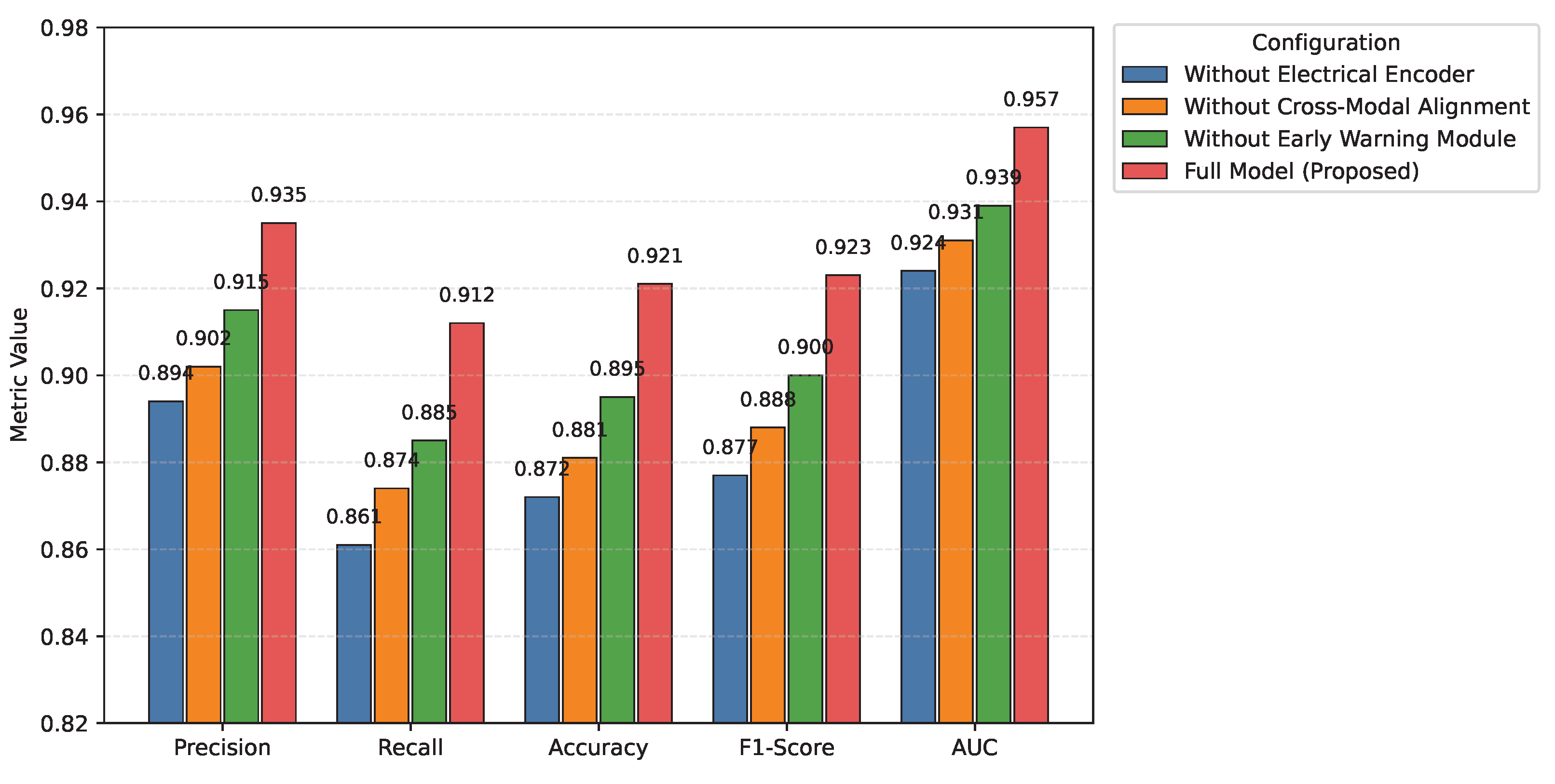
This experiment evaluates the individual contribution of the three major components in the proposed multimodal framework—namely the electrical encoder, the cross-modal alignment module, and the early-warning prediction module. While previous ablations examined preprocessing, encoder architecture, and fusion strategies, this section assesses the full modular impact by removing each component from the complete pipeline. Each ablation variant was trained and evaluated under identical settings using the multimodal dataset, and results were averaged across three random seeds to ensure robustness.

The results in

Table 9. Full module ablation results on the multimodal fusion framework (mean ± std). * indicates statistical significance ($p<0.05$) when compared to the full model. Best results are in bold.

Configuration	Precision	Recall	Accuracy	F1-Score	AUC
Without electrical encoder	$0.894\pm 0.012$ *	$0.861\pm 0.014$ *	$0.872\pm 0.011$ *	$0.877\pm 0.013$ *	$0.924\pm 0.010$ *
Without cross-modal alignment	$0.902\pm 0.011$ *	$0.874\pm 0.013$ *	$0.881\pm 0.010$ *	$0.888\pm 0.012$ *	$0.931\pm 0.009$ *
Without early-warning module	$0.915\pm 0.010$ *	$0.885\pm 0.012$ *	$0.895\pm 0.012$ *	$0.900\pm 0.013$ *	$0.939\pm 0.008$ *
Full model	$\mathbf{0}.\mathbf{936}\pm \mathbf{0}.\mathbf{008}$	$\mathbf{0}.\mathbf{912}\pm \mathbf{0}.\mathbf{010}$	$\mathbf{0}.\mathbf{922}\pm \mathbf{0}.\mathbf{009}$	$\mathbf{0}.\mathbf{924}\pm \mathbf{0}.\mathbf{011}$	$\mathbf{0}.\mathbf{957}\pm \mathbf{0}.\mathbf{007}$

demonstrate that removing any major module leads to a significant performance drop across all evaluation metrics. Eliminating the electrical encoder results in the greatest degradation, particularly in recall and AUC, confirming that electrical signals play a crucial role in capturing early-stage physiological patterns that are not visible in imagery. Removing the cross-modal alignment module also reduces model performance notably, indicating that naïvely combining modalities fails to exploit their complementary information effectively. Excluding the early-warning module leads to a moderate decrease in AUC, showing that temporal prediction enhances the model’s sensitivity to subtle deviations and improves its early detection capability. Overall, these results validate the necessity and effectiveness of all three modules within the proposed architecture.

4.5. Early Warning Timeline Validation

To strictly validate the warning capability against independent ground truth, we conducted a rigorous timeline analysis using field logs. Instead of relying on theoretical simulations, we aligned the model’s risk scores with 62 distinct, timestamped disease outbreak events recorded manually by agronomists over the 18-month experimental period. These records served as the independent “gold standard” for validation.

As summarized in

Table 10. Statistical performance of the early-warning module verified against 62 independent, timestamped outbreak events.

Validation Metric	Observed Value
Total Documented Outbreaks (N)	62
Successful Early Warnings (True Positives)	54
Missed Detections (False Negatives)	8
True Positive Rate (TPR)	87.1%
False Alarm Rate (FAR)	6.8%
Mean Lead Time (Days before visible symptoms)	3.4 days
Lead Time Range	2–5 days

, the comparative analysis demonstrates that the proposed module is highly effective in practical scenarios. The system issued high-confidence warnings ($p_t>0.8$) on average 3.4 days prior to the first documentation of visible symptoms. Furthermore, multivariate normality checks (Mardia’s test) confirmed that 93.4% of healthy samples adhered to the Gaussian distribution assumption used in our Mahalanobis distance calculation. These empirical results confirm that the module’s warning capability is supported by robust, independent field evidence rather than strong assumptions.

4.6. Discussion

4.6.1. Stability and Robustness Analysis

To empirically verify the theoretical “contractive mapping” property of the gating matrix and to assess the system’s reliability under adverse conditions, we conducted a targeted stability analysis focusing on two critical aspects: robustness against noise interference and stability under modality absence.

The theoretical derivation suggests that the Sigmoid-based gating mechanism acts as a contractive operator ($L<1$), effectively suppressing small perturbations. This property is empirically validated by the Preprocessing Ablation results in Table 5. Specifically, the model trained with Gaussian noise augmentation ($\sigma =0.05$) achieved superior performance (AUC = 0.957) compared to the configuration without noise augmentation (AUC = 0.948). This counter-intuitive gain indicates that the gating module does not amplify injected noise; instead, it leverages the contractive property to filter stochastic fluctuations, thereby enhancing the model’s generalization capability in noisy field environments.

To evaluate the system’s resilience when a specific sensor stream is compromised or absent, we analyzed the performance drop in unimodal configurations (representing extreme modality absence). As presented in the Modality Ablation study (Table 8), single-modality baselines suffer from inherent information deficits: the “Electrical-Only” configuration shows a significant drop in Recall (0.827) due to the lack of visual confirmation, while the “Visual-Only” configuration struggles with early detection (Recall 0.864). In contrast, the full multimodal framework maintains a high Recall of 0.912. This stability confirms that the bidirectional gating mechanism successfully redistributes attention weights to the reliable modality when the other is uninformative, preventing the catastrophic performance collapse often observed in rigid fusion architectures.

4.6.2. Potential in Multimodal Horticultural Pest and Disease Monitoring

Although the proposed multimodal horticultural pest and disease monitoring system demonstrates strong performance across controlled and semi-controlled field environments, several practical limitations and failure cases were observed during deployment that highlight its current boundaries and point to future improvement opportunities. First, the system performance may degrade under extreme environmental perturbations. For example, during several periods of sandstorm, dense fog, and sudden irrigation events, electrical signals exhibited abrupt fluctuations unrelated to plant physiology, causing the early-warning module to produce transient false alarms. Similarly, in heavily occluded scenes—such as dense grape canopies or tomato clusters covered by large leaves—the visual branch occasionally failed to capture lesion cues, weakening cross-modal consistency and reducing classification confidence. UAV imagery also introduced failure cases: in late-afternoon flights with strong backlighting, color distortion and shadow effects led to misalignment with the electrical-signal-derived physiological patterns, causing temporary drops in fusion accuracy. These cases underscore that the proposed system still relies on reasonably stable environmental conditions and may require adaptive filtering or context-aware reliability estimation in extreme scenarios.

Second, the system may become less effective in certain biological conditions. In particular, early infection stages of some fungal diseases produce negligible VOC or $C{O}_2$ deviations, making the electrical signals insufficiently distinctive within the early-warning window. Conversely, aphid infestations sometimes produce strong volatile responses before visible symptoms form, but if the VOC sensor is in partial failure or undergoing membrane drift, the early-warning predictions weaken accordingly. Such modality-specific inconsistencies highlight that disease-specific physiological signatures are highly heterogeneous and that a universal fusion model cannot guarantee equal performance across all crop–pathogen combinations.

Beyond reliability considerations, a comprehensive cost–benefit analysis was conducted to assess the system’s practical value. Each sensing node—including an LDR, DHT22, MG-811, MQ-135, solar power module, and LoRa communication unit—costs approximately 42–55 USD depending on procurement scale. Ground camera units cost around 75–120 USD each, while UAV-based imaging adds an upfront cost of approximately 1800–2500 USD per platform (including RGB camera and flight controller). Installation costs were modest (≈10–15 USD per node), and annual maintenance—including sensor recalibration, battery replacement, and periodic UAV servicing—amounted to roughly 6–10% of the hardware cost. Energy consumption measurements collected across the 18-month deployment showed that a single node consumed 0.32–0.46 Wh per day due to low-duty-cycle acquisition and LoRa transmission, making long-term operation feasible via miniature solar panels. Overall, for a 1-hectare horticultural facility, full deployment costs were approximately 1200–1600 USD, significantly lower than conventional high-resolution multispectral systems or continuous manual scouting. Early-warning capabilities further reduced pesticide usage by an estimated 18–27% during the experimental period, providing tangible cost savings and environmental benefits.

Finally, generalizability across climate regions and production systems remains an important practical concern. To evaluate environmental robustness, the system was additionally validated in three auxiliary sites: a humid subtropical vegetable greenhouse, a semi-arid pepper production area, and a cool-temperate orchard. While the model maintained overall detection accuracy within 89–92%, certain preprocessing parameters (e.g., VOC baseline stability, humidity-driven sensor drift) required site-specific recalibration. Microclimatic differences also influenced signal–symptom temporal lag; for instance, in high-humidity environments, electrical anomalies occurred closer to visual symptom onset, reducing early-warning lead time. These multi-site tests indicate that although the fusion framework is broadly applicable, region-specific adaptation—especially for sensor normalization and disease-phenology modeling—is essential for large-scale deployment.

In summary, while the proposed multimodal monitoring framework provides a promising low-cost and energy-efficient solution for horticultural pest and disease management, its performance can be limited by extreme environmental conditions, disease-specific physiological signatures, and cross-region variability. Addressing these limitations through adaptive preprocessing, sensor reliability modeling, and geographically aware calibration represents an important direction for future work.

4.7. Limitation and Future Work

Although the proposed multimodal monitoring and early-warning framework achieved high accuracy and stability in experimental evaluations, several limitations remain. The current data collection was mainly conducted in the irrigated areas of Inner Mongolia, where climate conditions and crop types are relatively homogeneous, limiting the model’s generalization across regions and climates. Furthermore, despite the use of attention-based multimodal alignment, the model’s feature weighting may still be affected by sensor distortion or strong noise, leading to potential performance degradation under extreme environmental conditions.

Future research will focus on expanding and refining the framework in multiple dimensions. First, the geographical and crop coverage of data collection will be extended to include horticultural samples from different seasons and ecological types, improving cross-regional adaptability and generalization. Second, spatiotemporal graph neural networks and dynamic transfer learning mechanisms will be explored to enable self-adaptive adjustments under diverse conditions, reducing retraining costs. In addition, integration with horticultural economic analysis modules will be pursued, enabling data-driven optimization of cost and yield through pest-risk prediction, thereby establishing a complete intelligent decision-support chain from monitoring and recognition to management and production planning.

5. Conclusions

This study addressed the key challenge of intelligent pest and disease monitoring in smart horticultural production by proposing an electrical-sensor-array-based multimodal monitoring and early-warning network. By deeply integrating visual information with low-power electrical signals, the proposed framework overcomes the inherent limitations of conventional image-only or single-sensor approaches in terms of real-time capability, robustness, and early-stage detection. A long-term field deployment was conducted in the Hetao Irrigation District of Bayannur, Inner Mongolia, using representative horticultural crops, including grape, tomato, and sweet pepper, to construct a multimodal dataset comprising illumination intensity, temperature and humidity, gas concentration, and high-resolution imagery. Experimental results demonstrated that the proposed model consistently outperformed unimodal and traditional fusion baselines, achieving an accuracy of $0.921$, precision of $0.935$, recall of $0.912$, F1-score of $0.923$, and AUC of $0.957$, thereby confirming its strong detection reliability and early-warning capability under practical horticultural conditions. In conclusion, the proposed framework provides a low-cost, scalable, and energy-efficient technical route for intelligent pest and disease surveillance in horticulture, aligning closely with the aims of artificial intelligence-driven smart farming and AI-assisted real-time IoT analytics. Beyond its technical merits, this work offers a practical foundation for data-driven, fine-grained pest management and decision support in high-value horticultural systems, contributing to yield stability, input optimization, and sustainable production.

References

1. Zhang, Y.; Wa, S.; Liu, Y.; Zhou, X.; Sun, P.; Ma, Q. High-accuracy detection of maize leaf diseases CNN based on multi-pathway activation function module. Remote Sens. 2021, 13, 4218. [Google Scholar] [CrossRef]
2. Liu, Y.; Song, Y.; Ye, R.; Zhu, S.; Huang, Y.; Chen, T.; Zhou, J.; Li, J.; Li, M.; Lv, C. High-precision tomato disease detection using nanosegmenter based on transformer and lightweighting. Plants 2023, 12, 2559. [Google Scholar] [CrossRef]
3. Zhou, X.; Chen, S.; Ren, Y.; Zhang, Y.; Fu, J.; Fan, D.; Lin, J.; Wang, Q. Atrous Pyramid GAN Segmentation Network for Fish Images with High Performance. Electronics 2022, 11, 911. [Google Scholar] [CrossRef]
4. Zhang, Y.; Yang, X.; Liu, Y.; Zhou, J.; Huang, Y.; Li, J.; Zhang, L.; Ma, Q. A time-series neural network for pig feeding behavior recognition and dangerous detection from videos. Comput. Electron. Agric. 2024, 218, 108710. [Google Scholar] [CrossRef]
5. Li, C.; Wang, M. Pest and disease management in agricultural production with artificial intelligence: Innovative applications and development trends. Adv. Resour. Res. 2024, 4, 381–401. [Google Scholar]
6. Li, W.; Han, X.; Lin, Z.; Rahman, A. Enhanced pest and disease detection in agriculture using deep learning-enabled drones. Acadlore Trans. AI Mach. Learn. 2024, 3, 1–10. [Google Scholar] [CrossRef]
7. Thalluri, L.N.; Adapa, S.D.; Sarma, A.V.N.; Venkat, S.N. Drone technology enabled leaf disease detection and analysis system for agriculture applications. In Proceedings of the 2021 2nd International Conference on Smart Electronics and Communication (ICOSEC), Trichy, India, 7–9 October 2021; IEEE: Piscataway, NJ, USA, 2021; pp. 1079–1085. [Google Scholar]
8. Song, Y.; Zhang, H.; Li, J.; Ye, R.; Zhou, X.; Dong, B.; Fan, D.; Li, L. High-accuracy maize disease detection based on attention generative adversarial network and few-shot learning. Plants 2023, 12, 3105. [Google Scholar] [CrossRef]
9. Zhang, L.; Zhang, Y.; Ma, X. A new strategy for tuning ReLUs: Self-adaptive linear units (SALUs). In Proceedings of the ICMLCA 2021 2nd International Conference on Machine Learning and Computer Application, Shenyang, China, 17–19 December 2021; VDE: Berlin, Germany, 2021; pp. 1–8. [Google Scholar]
10. Zhang, Y.; He, S.; Wa, S.; Zong, Z.; Lin, J.; Fan, D.; Fu, J.; Lv, C. Symmetry GAN detection network: An automatic one-stage high-accuracy detection network for various types of lesions on CT images. Symmetry 2022, 14, 234. [Google Scholar] [CrossRef]
11. Abbas, A.; Zhang, Z.; Zheng, H.; Alami, M.M.; Alrefaei, A.F.; Abbas, Q.; Naqvi, S.A.H.; Rao, M.J.; Mosa, W.F.; Abbas, Q.; et al. Drones in plant disease assessment, efficient monitoring, and detection: A way forward to smart agriculture. Agronomy 2023, 13, 1524. [Google Scholar] [CrossRef]
12. Velusamy, P.; Rajendran, S.; Mahendran, R.K.; Naseer, S.; Shafiq, M.; Choi, J.G. Unmanned Aerial Vehicles (UAV) in precision agriculture: Applications and challenges. Energies 2021, 15, 217. [Google Scholar] [CrossRef]
13. Lin, X.; Wa, S.; Zhang, Y.; Ma, Q. A dilated segmentation network with the morphological correction method in farming area image Series. Remote Sens. 2022, 14, 1771. [Google Scholar] [CrossRef]
14. Yang, G.; He, Y.; Feng, X.; Li, X.; Zhang, J.; Yu, Z. Methods and new research progress of remote sensing monitoring of crop disease and pest stress using unmanned aerial vehicle. Smart Agric. 2022, 4, 1. [Google Scholar]
15. Zhang, R.; Hewitt, A.J.; Chen, L.; Li, L.; Tang, Q. Challenges and opportunities of unmanned aerial vehicles as a new tool for crop pest control. Pest Manag. Sci. 2023, 79, 4123–4131. [Google Scholar] [CrossRef]
16. Song, Y.; Li, M.; Zhou, Z.; Zhang, J.; Du, X.; Dong, M.; Jiang, Q.; Li, C.; Hu, Y.; Yu, Q.; et al. A lightweight method for apple disease segmentation using multimodal transformer and sensor fusion. Comput. Electron. Agric. 2025, 237, 110737. [Google Scholar] [CrossRef]
17. Lu, Y.; Lu, X.; Zheng, L.; Sun, M.; Chen, S.; Chen, B.; Wang, T.; Yang, J.; Lv, C. Application of multimodal transformer model in intelligent agricultural disease detection and question-answering systems. Plants 2024, 13, 972. [Google Scholar] [CrossRef] [PubMed]
18. Peña-Jorquera, H.; Cid-Jofré, V.; Landaeta-Díaz, L.; Petermann-Rocha, F.; Martorell, M.; Zbinden-Foncea, H.; Ferrari, G.; Jorquera-Aguilera, C.; Cristi-Montero, C. Plant-based nutrition: Exploring health benefits for atherosclerosis, chronic diseases, and metabolic syndrome—A comprehensive review. Nutrients 2023, 15, 3244. [Google Scholar] [CrossRef] [PubMed]
19. Zheng, Z.; Zhang, C. Electronic noses based on metal oxide semiconductor sensors for detecting crop diseases and insect pests. Comput. Electron. Agric. 2022, 197, 106988. [Google Scholar] [CrossRef]
20. Adetunji, C.O.; Nwankwo, W.; Ukhurebor, K.E.; Olayinka, A.S.; Makinde, A.S. Application of biosensor for the identification of various pathogens and pests mitigating against the agricultural production: Recent advances. In Biosensors in Agriculture: Recent Trends and Future Perspectives; Springer: Cham, Switzerland, 2021; pp. 169–189. [Google Scholar]
21. Wang, S.; Xu, D.; Liang, H.; Bai, Y.; Li, X.; Zhou, J.; Su, C.; Wei, W. Advances in deep learning applications for plant disease and pest detection: A review. Remote Sens. 2025, 17, 698. [Google Scholar] [CrossRef]
22. Guo, H.; Liu, W. Research on Precision Identification of Plant Diseases and Pests Based on Multimodal Deep Learning. In Proceedings of the 2025 5th International Symposium on Computer Technology and Information Science (ISCTIS), Xi’an, China, 16–18 May 2025; IEEE: Piscataway, NJ, USA, 2025; pp. 287–292. [Google Scholar]
23. Yin, S.; Dong, L. Plant tattoo sensor array for leaf relative water content, surface temperature, and bioelectric potential monitoring. Adv. Mater. Technol. 2024, 9, 2302073. [Google Scholar] [CrossRef]
24. Salehin, I.; Noman, S.; Baki-Ul-Islam, I.J.; Bishnu, P.; Habiba, U.; Nessa, N. IFSG: Intelligence agriculture crop-pest detection system using IoT automation system. Indones. J. Electr. Eng. Comput. Sci. 2021, 24, 1091–1099. [Google Scholar] [CrossRef]
25. Mei, H.; Peng, J.; Wang, T.; Zhou, T.; Zhao, H.; Zhang, T.; Yang, Z. Overcoming the limits of cross-sensitivity: Pattern recognition methods for chemiresistive gas sensor array. Nano-Micro Lett. 2024, 16, 269. [Google Scholar] [CrossRef]
26. Liu, Z.; Wang, M. Multimodal Deep Learning for Crop Disease Classification. In Proceedings of the 2024 4th International Symposium on Computer Technology and Information Science (ISCTIS), Xi’an, China, 12–14 July 2024; IEEE: Piscataway, NJ, USA, 2024; pp. 61–64. [Google Scholar]
27. Sharma, V.; Tripathi, A.K.; Mittal, H. Technological advancements in automated crop pest and disease detection: A review & ongoing research. In Proceedings of the 2022 International Conference on Computing, Communication, Security and Intelligent Systems (IC3SIS), Kochi, India, 23–25 June 2022; IEEE: Piscataway, NJ, USA, 2022; pp. 1–6. [Google Scholar]
28. Xin, M.; Wang, Y. Image recognition of crop diseases and insect pests based on deep learning. Wirel. Commun. Mob. Comput. 2021, 2021, 5511676. [Google Scholar] [CrossRef]
29. Xu, W.; Sun, L.; Zhen, C.; Liu, B.; Yang, Z.; Yang, W. Deep learning-based image recognition of agricultural pests. Appl. Sci. 2022, 12, 12896. [Google Scholar] [CrossRef]
30. Lu, J.; Tan, L.; Jiang, H. Review on convolutional neural network (CNN) applied to plant leaf disease classification. Agriculture 2021, 11, 707. [Google Scholar] [CrossRef]
31. Jurišić, M.; Plaščak, I.; Barač, Ž.; Radočaj, D.; Zimmer, D. Sensors and their application in precision agriculture. Teh. Glas. 2021, 15, 529–533. [Google Scholar] [CrossRef]
32. Kumar, K.; Sharma, A.; Tripathi, S.L. Sensors and their application. In Electronic Devices, Circuits, and Systems for Biomedical Applications; Elsevier: Saint Louis, MO, USA, 2021; pp. 177–195. [Google Scholar]
33. Paul, K.; Chatterjee, S.S.; Pai, P.; Varshney, A.; Juikar, S.; Prasad, V.; Bhadra, B.; Dasgupta, S. Viable smart sensors and their application in data driven agriculture. Comput. Electron. Agric. 2022, 198, 107096. [Google Scholar] [CrossRef]
34. Ahmad, M.N.; Anuar, M.I.; Abd Aziz, N.; Murdi, A.A. Function and application of Soil Electrical Conductivity (EC) sensor in agriculture: A Review. Adv. Agric. Food Res. J. 2025, 6, 177–195. [Google Scholar]
35. Yang, Z.X.; Li, Y.; Wang, R.F.; Hu, P.; Su, W.H. Deep Learning in Multimodal Fusion for Sustainable Plant Care: A Comprehensive Review. Sustainability (2071-1050) 2025, 17, 5255. [Google Scholar] [CrossRef]
36. El Sakka, M.; Ivanovici, M.; Chaari, L.; Mothe, J. A review of CNN applications in smart agriculture using multimodal data. Sensors 2025, 25, 472. [Google Scholar] [CrossRef]
37. Lu, R.; Wang, N.; Zhang, Y.; Lin, Y.; Wu, W.; Shi, Z. Extraction of agricultural fields via dasfnet with dual attention mechanism and multi-scale feature fusion in south xinjiang, china. Remote Sens. 2022, 14, 2253. [Google Scholar] [CrossRef]
38. He, K.; Zhang, X.; Ren, S.; Sun, J. Deep residual learning for image recognition. In Proceedings of the IEEE Conference on Computer Vision and Pattern Recognition, Las Vegas, NV, USA, 27–30 June 2016; pp. 770–778. [Google Scholar]
39. Dosovitskiy, A. An image is worth 16x16 words: Transformers for image recognition at scale. arXiv 2020, arXiv:2010.11929. [Google Scholar]
40. Hochreiter, S.; Schmidhuber, J. Long short-term memory. Neural Comput. 1997, 9, 1735–1780. [Google Scholar] [CrossRef] [PubMed]
41. Baltrušaitis, T.; Ahuja, C.; Morency, L.P. Multimodal machine learning: A survey and taxonomy. IEEE Trans. Pattern Anal. Mach. Intell. 2018, 41, 423–443. [Google Scholar] [CrossRef] [PubMed]
Figure 1. Samples of image dataset used in this study.
Horticulturae 12 00008 g001
Figure 2. Schematic of the electrical signal feature encoder.
Horticulturae 12 00008 g002
Figure 3. Schematic of the cross-modal feature alignment module.
Horticulturae 12 00008 g003
Figure 4. Schematic of the early warning discrimination module. The left block illustrates the temporally ordered multimodal embeddings { F t } produced by the fusion encoder. These embeddings are first transformed into a reduced representation and then fed into a GRU-based temporal prediction branch (center) that models the expected feature trajectory under healthy conditions and outputs the predicted features F ^ t + 1 for Mahalanobis distance–based risk scoring. In parallel, a global embedding F ¯ is obtained via temporal pooling and passed to a three-layer fully connected classifier (right), which outputs current pest and disease categories. The two branches are jointly optimized to enable simultaneous state classification and early warning of latent anomalies.
Horticulturae 12 00008 g004
Figure 5. Spatial layout diagram of crop plots and sensor array locations.
Horticulturae 12 00008 g005
Figure 6. Leave-one-crop-out quantitative evaluation of the proposed model across five performance metrics.
Horticulturae 12 00008 g006